StartAbility GradeAbility Acceleration Capacity Overtaking provision Tracking Ability Straight Path Ride quality Low Speed Swept path Friction Demand on Steer Tyre Static Rollover Threshold Rearward Amplification, High speed off-tracking
Yaw Damping Handling Quality Directional Stability while Braking Cross-Wind Sensitivity
An Open Assessment Tool for
Performance Based Standards of
Long Combination Vehicles
Research report
Research report
An Open Assessment Tool for Performance Based
Standards of Long Combination Vehicles
Bengt Jacobson, Peter Sundström, Sogol Kharrazi, Niklas Fröjd, Manjurul Islam
Department of Mechanical and Maritime sciences Division of Vehicle Engineering and Autonomous Systems
Vehicle Dynamics group
CHALMERS UNIVERSITY OF TECHNOLOGY Göteborg, Sweden 2017
An Open Assessment Tool for Performance Based Standards of Long Combination Vehicles Bengt Jacobson, Peter Sundström, Sogol Kharrazi, Niklas Fröjd, Manjurul Islam
© Bengt Jacobson, Peter Sundström, Sogol Kharrazi, Niklas Fröjd, Manjurul Islam, 2017-08-31
Research report 2017:03
Department of Mechanical and Maritime sciences
Division of Vehicle Engineering and Autonomous Systems Vehicle Dynamics group
Chalmers University of Technology
SE-412 96 Göteborg
Sweden
Telephone: + 46 (0)31-772 1000
Picture on cover page: Illustration of one set of PBSes, from Joop Pauwelussen and Karel Kural, HAN University of Applied Sciences, The Netherlands.
Chalmers University of Technology, Göteborg, Sweden 2017-08-31
An Open Assessment Tool for Performance Based Standards of Long Combination Vehicles
Research report
Bengt Jacobson, Peter Sundström, Sogol Kharrazi, Niklas Fröjd, Manjurul Islam
Department of Mechanical and Maritime sciences,
Division of Vehicle Engineering and Autonomous Systems,
Vehicle Dynamics group,
Chalmers University of Technology
Abstract
The project “Performance Based Standards for High Capacity Transports in Sweden” [1] have generated a first beta version of an open PBS assessment tool, OpenPBS. The tool uses models and computations to calculate Performance Based Standards (PBS) measures for combination vehicles. The tool targets Long Combination Vehicles (LCVs, typically 25-35 m long) but it can also calculate PBSes for shorter combinations and solo units. This report explains the concepts selected for the tool. Finally, future developments are proposed.
Keywords
High capacity transports, Long combination vehicles, Performance based standards, Open source, Assessment tool, Modelica, FMU
Acknowledgements
Authors are thankful to FFI & Vinnova, which funded the project “Performance Based Standards for High Capacity Transports in Sweden” (FFI project, Vinnova reference number 2013-03881) whereof the results in this paper is a result.
Authors: Bengt Jacobson (Chalmers), Peter Sundström (Modelon), Sogol Kharrazi (VTI), Niklas Fröjd (Volvo GTT), Manjurul Islam (Chalmers)
Contents
Abstract ... 5 Keywords ... 5 Acknowledgements ... 5 Contents ... 6 1 Introduction ... 7 1.1 Background ... 7 1.1.1 Project ... 7 1.2 Problem ... 7 1.3 Envisioned solution ... 7 1.4 Objective ... 91.5 Requirements on the tool ... 9
2 Tool ... 10
2.1 Overall structure ... 10
2.1.1 VehicleParameters... 10
2.1.2 VehicleModels... 10
2.1.3 Manoeuvres ... 12
2.1.4 Components and Sandbox ... 13
2.2 Implementation of each PBS ... 13
2.3 Implementation of each Manoeuvre ... 15
2.3.1 Longitudinal ... 15
2.3.2 LowSpeedCurve ... 16
2.3.3 LowSpeedCurve,_SaturatedTyres ... 16
2.3.4 HighSpeedStraightPath... 17
2.3.5 HighSpeedCurve: ... 18
2.3.6 SteadyStateRollOver <Only implemented as placeholder> ... 18
2.3.7 BrakingStabilityInTurn <Only implemented as placeholder> ... 19
2.3.8 Selection between SingleLaneChange and SingleSineSteering ... 20
2.3.9 SingleLaneChange: ... 20
2.3.10 SingleSineSteering: ... 22
3 Example of usage ... 22
3.1 Finding design parameter envelopes for allowed combination vehicles ... 22
4 Conclusions ... 22
5 Future work ... 23
5.1 Tyre models ... 23
5.2 Active systems ... 23
5.3 Other requirements than present PBSes ... 23
1 Introduction
1.1 Background
Long Combination Vehicles (LCVs) are generally transport efficient, including energy efficient. However, there can be many designs of LVCs. In order to allow only suitable designs, authorities can base the legislation on Performance Based Standards (PBS).
Most of the existing legal requirements are requirements on each unit, not on a whole
combination vehicle. One PBS is a complementing requirement, motivated by additional risks identified for when one couple legal units to LVCs. For each region, there should be a set of PBSes which together covers these risks well. One single PBS is a well-defined measure of complete combination vehicles performance. Each PBS should have a numeric requirement level. The alternative to PBS would be to require certain design parameters, such as lengths, weights, etc. Table 1.1 show the set of PBSes proposed in present report. The picture on the cover illustrates a slightly different set of PBSes.
1.1.1 Project
A project called “Performance Based Standards for High Capacity Transports in Sweden” (FFI project, Vinnova reference number 2013-03881), see Reference [1] has proposed a set of PBSes with requirement levels for Sweden, see Table 1.1. The project has also proposed computational methods (models with simulations/computations) for virtual verification of these PBSes and implemented them in a computer tool. A first version of it is released as an open PBS assessment tool, “OpenPBS”, see https://github.com/performance-based-standards/OpenPBS. Present report describes this tool.
In connection to the project, Swedish Transport Agency has worked on a web-application for approval of individual combination vehicles. The tool presented in present report is, so far, not used by the web-application, but could be in future version.
1.2 Problem
Even if there are standards, e.g. ISO, which defines measures that could be used as PBS measures, different assessors will come to different numerical values depending on details in interpretation of the standards. Additional differences appears due to differences in how vehicles and manoeuvres are parameterised and modelled (for virtual assessment, i.e. via computation) and test conditions etc. (for real assessment, i.e. via real vehicle tests).
1.3 Envisioned solution
An envisioned solution to the problem is to develop an open (free, readable and understandable) assessment tool. Such tool has to be based on standard formats for dynamic models. Modelica [2] is proposed as such modelling format and FMI [3] is proposed as such execution format. These two formats are the only ones of their kinds which is agreed in a wide community. The tool need to support at least two different use cases:
Research and development of combination vehicles: Here, the Modelica format is suitable since it allows variations of both models (equations) and all parameters. Legislation for allowing/forbidding certain types or individuals of combination
vehicles: Here, the FMU format is suitable since it can give stable simulation models
with only a selected limited set of parameters accessible for variation.
The openness of such tool should be such that it reveals the exact models (equations and parameters, including how the PBS measures are calculated). This has the additional benefit of defining the manoeuvres in an unambiguous way (how to drive the vehicles, how to load them, on which road friction, etc.). That is very useful also for real vehicle assessment.
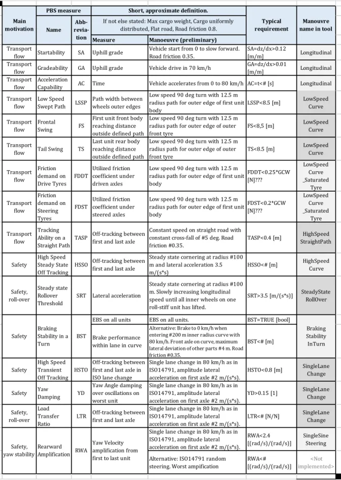
Table 1.1: The set of PBSes from project “Performance Based Standards for High Capacity Transports in Sweden” (FFI project, Vinnova reference number 2013-03881).
Measure Manoeuvre (preliminary)
Transport
flow Startability SA Uphill grade
Vehicle start from 0 to slow forward. Road friction 0.35.
SA=dz/dx>0.12
[m/m] Longitudinal Transport
flow Gradeability GA Uphill grade Vehicle drive in 70 km/h
GA=dz/dx>0.01
[m/m] Longitudinal Transport
flow
Acceleration
Capability AC Time Vehicle accelerates from 0 to 80 km/h AC=t<# [s] Longitudinal Transport
flow
Low Speed Swept Path LSSP
Path width between wheels outer edges
Low speed 90 deg turn with 12.5 m radius path for outer edge of first unit body LSSP<8.5 [m] LowSpeedCurve Transport flow Frontal Swing FS
First unit front body reaching distance outside defined path
Low speed 90 deg turn with 12.5 m radius path for outer edge of outer front tyre
FS<8,5 [m] LowSpeed Curve Transport
flow Tail Swing TS
Last unit rear body reaching distance outside defined path
Low speed 90 deg turn with 12.5 m radius path for outer edge of outer front tyre TS<8.5 [m] LowSpeedCurve Transport flow Friction demand on Drive Tyres FDDT Utilized friction coefficient under driven axles
Low speed 90 deg turn with 12.5 m radius path for outer edge of first unit body FDDT<0.25*GCW [N]??? LowSpeed Curve _Saturated Tyre Transport flow Friction demand on Steering Tyres FDST Utilized friction coefficient under steered axles
Low speed 90 deg turn with 12.5 m radius path for outer edge of first unit body FDST<0.2*GCW [N]??? LowSpeed Curve _Saturated Tyre Transport flow Tracking Ability on a Straight Path
TASP Off-tracking between first and last axle
Constant speed on straight road with constant cross-fall of #5 deg. Road friction #0.35. TASP<0.4 [m] HighSpeed StraightPath Safety High Speed Steady State Off Tracking
HSSO Off-tracking between first and last axle
Steady state cornering at radius #100 m and lateral acceleration 3.5 m/(s*s) HSSO<# [m] HighSpeed Curve Safety, roll-over Steady state Rollover Threshold SRT Lateral acceleration
Steady state cornering at radius #100 m. Slowly increasing longitudinal speed until all inner wheels on one roll-stiff unit has lifted.
SRT>3.5 [m/(s*s)] SteadyState RollOver EBS on all units EBS on all units. BST=TRUE [bool]
Brake performance within lane in curve
Alternative: Brake to 0 km/h when entering #200 m inner radius curve with 80 km/h. Front axle on curve, maximum lateral deviation of other parts #4 m. Road friction #0.35. BST<# [m] Safety High Speed Transient Off Tracking HSTO Off-tracking between first and last axle in ISO lane change
Single lane change in 80 km/h as in ISO14791, amplitude lateral acceleration on first axle #2 m/(s*s).
HSTO<0.8 [m] SingleLane Change Safety Yaw Damping YD
Yaw Angle damping over oscillations on worst unit
Single lane change in 80 km/h as in ISO14791, amplitude lateral acceleration on first axle #2 m/(s*s).
YD>0.15 [1] SingleLaneChange Safety, roll-over Load Transfer Ratio LTR Off-tracking between first and last axle
Single lane change in 80 km/h as in ISO14791, amplitude lateral acceleration on first axle #2 m/(s*s).
LTR<# [N/N] SingleLane Change Single lane change in 80 km/h as in
ISO14791, amplitude lateral acceleration on first axle #2 m/(s*s).
RWA<2.4 [(rad/s)/(rad/s)]
SingleSine Steering Alternative: ISO14791 random
steering. Worst ampification
RWA<# [(rad/s)/(rad/s)] <Not implemented> Manouvre name in tool Braking Stability InTurn PBS measure Abb- revia-tion Name Typical requirement Yaw Velocity amplification from first to last unit
Main motivation
Short, approximate definition.
If not else stated: Max cargo weight, Cargo uniformly distributed, Flat road, Road friction 0.8.
BST Braking Stability in a Turn Safety Safety, yaw stability Rearward Amplification RWA
There are already assessment tools for PBSes, but these are not open. Instead, they are intellectual property for the assessors. An example of such assessor is the Australian Road Research Board (http://www.arrb.com.au/).
PBS for LCV has been addressed in many projects and papers, but compiling it to an executable and open tool, in widely accepted standard formats for dynamic models, is novel.
1.4 Objective
The objective behind the work presented in present report is to develop a first version of an Open PBS assessment tool. All PBSes (according to project [1]) should be implemented, while only some combination vehicles can be implemented (because there is no way to cover all future vehicles). The sample implemented vehicles are: A-double, Nordic combination and Tractor-Semitrailer.
1.5 Requirements on the tool
One basic guiding principle has been to keep vehicle definition (vehicle design parameters) independent from definitions of PBS measures/manoeuvres, so that any vehicle can be assessed in the same way. This is important to enable future vehicle development.
Another basic guiding principle has been to keep vehicle definition independent from vehicle
model, so that vehicle models can be changed over time when/if motivated. This means that
vehicle model parameters and vehicle model equations are defined as independently as possible from each other.
A concept for propagating vehicle design parameters is an important part of the outline, both for securing that same vehicle is assessed in all PBSs and, in a continuation, for fetching
parameters from a data base/vehicle registry. In such registry, typically each unit is defined as opposed to each combination vehicles.
Simplest possible vehicle models has to be strived for to facilitate parametrisation and
understanding. The simplicity is limited by that variation of each vehicle parameter shall predict a variation of PBS measures accurate enough. Required accuracy is difficult to quantify, but it should be noted that it is much lower than corresponding requirements for high fidelity models used for, e.g. vehicle development at vehicle manufacturers.
Simplest possible PBS measure/manoeuvre models (or executable experiments) also has to
be strived for, again to facilitate parametrisation and understanding. This simplicity is limited by that all legislating authorities (e.g. in different countries/different road networks) should be able to represent their specific conditions (such as low/high road friction) and their specific
requirement levels. This paper does not claim to have fulfilled this, since focusing on Swedish conditions, but it has been in the mind-set when outlining the tool.
Descriptions of the PBSs is essential to keep in the tool itself, to avoid divergence over time.
There should be traffic situation based motivations to each PBS, typical numerical requirement levels and drawings explaining the manoeuvres and measures. When understanding the whole set of PBSes one have to remember that the PBSes commonly addresses a set of “risks”,
represented by the traffic situations, which are found relevant for long combination vehicles. The overall requirement on computational efficiency is not very limiting, such as no requirement on real time simulation. However, a typical use case within research and development is to optimize or sweep over large vehicle design parameter spaces, which calls for assessment of all PBSes for one vehicle in the order of magnitude of 1..10 ms on a typical PC of today.
Many limitations has been done. The most important are mentioned as proposals for future work in Section “5 Future work”. One limitation to especially mention would be that “active systems” is not considered. By “active systems” is then meant algorithm based brake control, powertrain control, extra propelled axles, extra steered axles.
2 Tool
This section presents the tool. Please refer to Section “1.5 Requirements on the tool”.
2.1 Overall structure
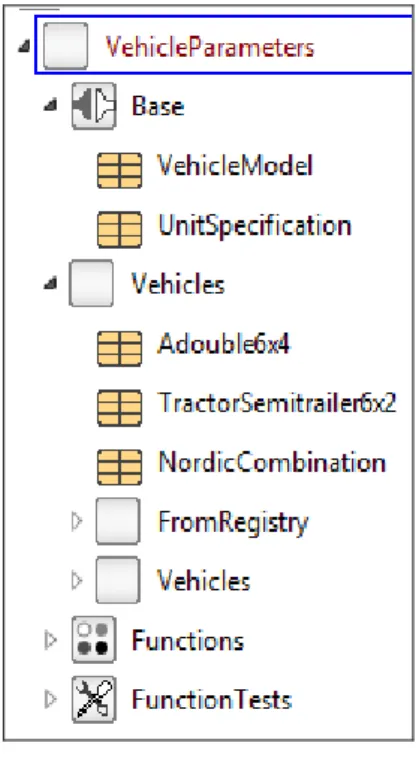
The tool is structured with Modelica packages. The root package opens with the Modelica file package.mo. Packages on root level are shown together in Figure 2-1 and described in Section2.1.1..0 0.
A visualization of the architecture is given in Figure 2-3.
Figure 2-1: Packages on root.
2.1.1 VehicleParameters
Package VehicleParameters contains registries (sets of parameters) which defines the vehicles in terms of vehicle parameters, such as wheelbase and kerb mass. Note that no vehicle equations are introduced so far.
As seen in Figure 2-3 and Figure 2-2, the concept is to differ between Unit specifications and Vehicle Specifications. This is mainly to prepare for:
Reading parameters from databases, such as vehicle manufacturers databases and authorities vehicle registries. UnitSpecification is declared for reading from databases. Such specifications are typically not complete for a simulation.
Handling such as kerb weight vs (pay-)load and different road friction, which could be different for different manoeuvres and PBSes for the same vehicle specification. VehicleModel (parameters) are declared and should be enough for simulation. A function, ModelParametersFromSpecification (shorted Unit2VehicleModel,in Figure 2-3) is defined. For instance, such as tyre lateral slip stiffness 𝐶𝑦 for each
axle is needed in the vehicle model. But it is seldom found in databases. So, a “reasonable standard value” on
cornering coefficient 𝐶𝐶𝑦 is used in the function, to specify
that 𝐶𝑦= 𝐶𝐶𝑦⋅ 𝐹𝑧 for each axle, where 𝐹𝑦 is the static vertical force on the axle; so it is dependent on (pay-)load.
Figure 2-2: Package VehicleParameters.
2.1.2 VehicleModels
Package VehicleModels contains equations defining the vehicle models, such as equations of motion and tyre constitutional equations. A registry from the previously described package is included in each vehicle model, so that the equations can use the vehicle parameters defined there and the vehicle parameters can be set for instances of the vehicle model. Note that the manoeuvre is not defined in the vehicle model.
fix some parameters record UnitSpec parameters L, m_kerb, m_load_max; called by parameterise via vehicle database pick in database (e.g. give unit
registration numbers)
function Unit2VehicleModel ”couples and assumes typical values on missing parameters”
record VehModSpec “vehicle design” extends UnitSpec;
parameter nu “number of units”, m_loaded;
parameters [nu, h, CC]= Unit2VehicleModel(unitSpec); extended by
instantiated in
model LongVehMod “vehicle behavior” parameter VehModSpec vehModSpec; parameter m_loaded;grade; equation
m_loaded*der(vx)=Fx-grade*m*g;
model Longitudinal”manoeuvre with some PBSes” VehModSpec vehModSpec;
parameter load=1, grade=0.05;
LongVehMod vehMod(VehModSpec=vehModSpec, m_load=m_kerb+load*m_load_max,grade=grade); Real GA, valid;
equation GA=…; valid=…; record Adouble = VehicleModel(nu=4, L=[4,7,5,7], CC=7.5, …);
parameterise, simulate, typically manual variation of design parameters generate FMU
Manoeuvers VehicleModels
VehicleParameters
file Longitudinal.fmu Analyse result. Take design decisions. … Allowed or not, total and on each PBS. Recommended actions, …
simulate compare with requirements
set required values on PBS meassures FMUs
parameterise, simulate, typically sweeping design parameters
Figure 2-3: Visualisation of the tool architecture. Dashed indicates not implemented and tested so far.
As seen in Figure 2-3 and Figure 2-4, there are several vehicle models. It is important to use as simple models as possible when it comes to parameterisation. On the other hand, if a parameter is needed for one Manoeuvre, it can as well be used in another Manoeuvre without increasing the complexity.
Only an approximate description of the vehicle models is given in this report, since they are likely to be topic for further development in future versions of the OpenPBS:
The model SingleTrack is used for lateral manoeuvres, both low speed and high speed. It is similar to the model presented in [4].
The model Longitudinal is built on similar concept, but captures only the longitudinal dynamics.
Both these models are vectorised, so they can represent any combination of several units, coupled with yaw moment free couplings. For both models, the (static) heave and pitch equilibria is added, so that (static) vertical loads on each axle is defined.
The selection of vehicle models are also discussed in Section 2.3.
2.1.3 Manoeuvres
Package Manoeuvres contains models where the vehicle models from the previously described package is instantiated. Manoeuvres parameters and equations are added as well as calculations of the PBS measures (each one only represented by a Modelica variable, named as the PBS’s name in Table 1.1) that can be found from the manoeuvre. A registry from the package described in section 2.1.1 is included in each manoeuvre model, to standardize which vehicle parameters to set in a Manoeuvre model. Note that the Manoeuvre models are complete in the meaning that they can be simulated; either directly in the Modelica tool or exported as FMUs for simulation in an arbitrary platform.
As seen in Figure 2-3 and Figure 2-5, there are some Manoeuvres, but less than number of PBSes.
The main approach is to make the Manoeuvres independent of vehicle. However, there are also some vehicle specific variants of the Manoeuvres, shown in Figure 2-5 but not in Figure 2-3. The vehicle specific Manoeuvres are desired to avoid, but was found necessary in some cases. The implementation is done with inheritance, so that e.g. SingleLaneChange in VehicleSpecific is an extension of the (vehicle independent) SingleLaneChange. In future versions of the OpenPBS, it should be sorted out whether both are needed.
Each PBS measure is a continuous output variable with unit. A boolean output variable “valid” is also calculated. It tells whether all the outputted PBS measures of the Manoeuvre are credible.
No required PBS value is implemented yet. If that is done, it would make sense to output also a boolean variable that tell if the LCV has passed or failed on each PBS.
Each Manoeuvre is further discussed in Section 2.2.
ve
hi
cl
e
in
de
pe
nde
n
t
ve
hic
le
s
pe
cif
ic
Figure 2-5: Package Manoeuvres.
The Manoeuvres are the models from which FMUs are generated. FMUs can be generated with different sets of FMU parameters (meaning that a FMU parameter is such that can be changed between executions of the FMU):
VehicleModel parameters or UnitSpecification parameters.
Parameters for the Manoeuvres can be FMU parameters, such as (pay-)load if that is not fixed in the actual Manoeuvre/PBS definition.
When using OpenPBS for Research & Development one might want to have full control of all parameters, so all
Modelica parameters can then be kept as FMU parameters. If the tool should be used for assessment based on
authorities’ vehicle registry, it can be suitable to keep only those parameters that actually are stored for each registered unit and, potentially, if other parameters such as (pay-)load, load height, road network, etc. should be input parameters for the assessment. Figure 2-6 shows an example of an authority assessment tool.
Figure 2-6: Screendump from a test version of an authority assessment tool.
2.1.4 Components and Sandbox
Package Components contains various models which are useful in the Manoeuvre Models. Package Sandbox contains models used for testing during tool development.
2.2 Implementation of each PBS
The definition/implementation of each PBS is listed in the section for the manoeuvre where the PBS is computed, in Section 2.3. But to understand why it is defined/implemented in a certain way, one have to first agree of the motivation why the PBS measure is proposed. And, to do that, it is important to see the whole set of motivations beside each other. Hence, Table 2.1 is
compiled.
Table 2.1: The set of PBSes from project “Performance Based Standards for High Capacity Transports in Sweden” (FFI project, Vinnova reference number 2013-03881).
PBS Motivation
SA
SA is motivated by the risk of that LVCs get stuck in uphill and thereby creates traffic congestion. It does not address limitation due to low tyre-to-road friction conditions.
GA
GA is motivated by the risk of that LVCs drives very slow in uphill and thereby creates traffic congestion.
PBS Motivation
AC
AC is motivated by the risk of that LVCs have to wait long time before entering a road with high traffic density and thereby create traffic congestions.
LSSP, FS, TS
LSSP, FS and TS are motivated by the risk of that LVCs cannot take narrow turns without interfering with obstacles laterally outside the road and thereby creates damages or traffic congestion. It does not address low tyre-to-road friction conditions, since that is covered by FDDT and FDST.
The manoeuvre is a 12.5 m outer radius and 90 degrees yawing at low speed.
FDDT, FDST
FDDT and FDST are motivated by the risk of that LVCs cannot take narrow turns due to low tyre-to-road friction and thereby creates traffic congestion.
The manoeuvre is a 12.5 m outer radius and 90 degrees yawing at low speed.
TASP
TASP is motivated by the risk of that LVCs deviate too much laterally when driving on relatively straight roads and thereby creates accidents.
HSSO
HSSO is motivated by the risk of that LVCs deviate too much laterally when driving in curves and thereby creates accidents.
SRT
SRT is motivated by the risk of that LVCs rolls over in long curves and thereby creates accidents.
BST
BST is motivated by the risk of that LVCs deviate too much laterally or have limited longitudinal brake performance when braking in curves when low tyre-to-road friction and thereby creates accidents.
HSTO
HSTO is motivated by the risk of that LVCs deviate too much laterally when changing lane and thereby creates accidents.
YD
YD is motivated by the risk of that LVCs becomes laterally unstable after changing lane and thereby creates accidents.
LTR
LTR is motivated by the risk of that LVCs rolls over when changing lane and thereby creates accidents.
RWA
RWA is motivated by the risk of that LVCs becomes difficult to manoeuvre laterally in high speed and thereby creates accidents.
2.3 Implementation of each Manoeuvre
The implementation of the PBS measures are a first proposal, so changes can be motivated in future versions of the OpenPBS. In the following section a brief description, organised for each manoeuvre, is given together with some thoughts of possible future studies or changes.
2.3.1 Longitudinal
0 4 8 12 16 20 0.20 0.24 S 0 4 8 12 16 20 0.04 0.05 G 0 4 8 12 16 20 0 20 AC 0 4 8 12 16 20 false true valid paramSet startability gradeability longitudin… distance_target > switch1 const k=0 const1 k=1 derivative I k=1 S G AC v alidFigure 2-7: Manoeuvre Longitudinal.
2.3.1.1 Startability SA [
𝒎𝒎]
SA is motivated by the risk of that LVCs get stuck in uphill and thereby creates traffic congestion. It does not address limitation due to low tyre-to-road friction
conditions.
The simplest possible model assumes that maximum tractive force at zero speed is a parameter in the vehicle specification. A typical rolling resistance coefficient of 0.004 is assumed. The computation becomes a pure algebraic computation, i.e. no simulation.
The propulsion system can limit SA also in ways that are more complex: limited by control limitations due to drive shaft loads, wear and fatigue on clutch and other propulsion system components. This is not modelled.
The statement above that limitation due to low tyre to road friction is not covered in present SA is now followed up: A European (not Swedish) requirement is to have >25% vertical load on driven axles. If applying that on LCVs would roughly limit Startability at low friction (𝜇 = 0.3) to 𝑆𝐴𝑙𝑜𝑤𝜇= tan(arcsin(𝜇 ⋅ 0.25)) = 0.075 [𝑚 𝑚⁄ ]. This should be compared to the requirement 𝑆𝐴 ≥ 0.12 [𝑚 𝑚⁄ ] in Table 1.1. A conclusion is that >25% vertical load on driven axles would allow severely reduced SA at low friction. This might call for a development of SA to be defined at low friction instead, so that the worst of propulsion and road grip on low friction determines the PBS.
See Modelica code for exact definition.
2.3.1.2 Gradeability GA [
𝒎𝒎]
GA is motivated by the risk of that LVCs drives very slow in uphill and thereby creates traffic congestion.
The simplest possible model assumes that maximum propulsion power is a parameter in vehicle specification. A typical frontal area and 𝑐𝑑 are assumed. The computation becomes a pure algebraic computation, i.e. no simulation.
See Modelica code for exact definition.
2.3.1.3 Acceleration Capability AC [𝒔]
AC is motivated by the risk of that LVCs have to wait long time before entering a road with high traffic density and thereby create traffic congestions.
This manoeuvre becomes a simulation, so pure algebraic computation is not enough. See Modelica code for exact definition.
2.3.2 LowSpeedCurve
LSSP, FS and TS are motivated by the risk of that LVCs cannot take narrow turns without interfering with obstacles laterally outside the road and thereby creates
damages or traffic congestion. It does not address low tyre-to-road friction conditions, since that is covered by FDDT and FDST.
The manoeuvre is a 12.5 m outer radius and 90 degrees yawing at low speed.
0 4 8 12 16 20 0 10 LSSP 0 4 8 12 16 20 0.0 0.2 FS 0 4 8 12 16 20 0.00 0.04 RS 0 4 8 12 16 20 false true valid TS TS pathPositi… pathPositi… const k=5 curve90deg[] curve90deg[] vehicle paramSet matrix(vehicle.vehicle.vy)*ones(1, na) realExpression3[] matrix(vehicle.vehicle.vy)*ones(1, na) realExpression3[] matrix(vehicle.vehicle.pz)*ones(1, na) realExpression4[] matrix(vehicle.vehicle.pz)*ones(1, na) realExpression4[] matrix(vehicle.vehicle.vx)*ones(1, na) realExpression5[] matrix(vehicle.vehicle.vx)*ones(1, na) realExpression5[] pathPositi… pathPositi… curve90deg1[] curve90deg1[] motionOffsetLeft[] motionOffsetLeft[] matrix(vehicle.vehicle.wz)*ones(1, na) realExpression7[] matrix(vehicle.vehicle.wz)*ones(1, na) realExpression7[] motionOffsetRight[] motionOffsetRight[] rollingMax curve_start + curve_radius*Modelica.Constants.pi/2 > rollingMax1 0.05 < and1 and overHang… overHang… matrix(vehicle.vehicle.vx)*ones(1, 2) realExpression9[] matrix(vehicle.vehicle.vx)*ones(1, 2) realExpression9[] matrix(vehicle.vehicle.vy)*ones(1, 2) realExpression10[] matrix(vehicle.vehicle.vy)*ones(1, 2) realExpression10[] matrix(vehicle.vehicle.wz)*ones(1, 2) realExpression11[] matrix(vehicle.vehicle.wz)*ones(1, 2) realExpression11[] matrix(vehicle.vehicle.pz)*ones(1, 2) realExpression12[] matrix(vehicle.vehicle.pz)*ones(1, 2) realExpression12[] rollingMax4 rollingMax5 LSSP v alid TS RS
Figure 2-8: Manouvre LowSpeedCurve.
2.3.2.1 Low Speed Swept Path LSSP [𝒎]
See Modelica code for exact definition.
2.3.2.2 Frontal swing FS [𝒎]
See Modelica code for exact definition.
2.3.2.3 Tail swing TS [𝒎]
See Modelica code for exact definition.
2.3.3 LowSpeedCurve,_SaturatedTyres
FDDT and FDST are motivated by the risk of that LVCs cannot take narrow turns due to low tyre-to-road friction and thereby creates traffic congestion.
The manoeuvre is a 12.5 m outer radius and 90 degrees yawing at low speed.
Reference [5] did a deep dive into the PBSes FDDT and FDST. It shows that one need to tyre models which can represent combined slip and saturation on the driven axles. On the non-driven axles, it is enough with lateral slip models, but saturation is needed, since the axle group on
towed units will saturate due to small turning radius. A road friction coefficient has to be numerically given (0.3 is presently used). The simulation gives one pass or fail result on FDDT and FDST, so it is essentially one PBS measure as it is coded now. Possibly, the coding could be developed, so that two continuous friction coefficient variables could be output, one for FDDT and one for FDST.
0 10 20 30 0.0 0.1 FDST 0 10 20 30 0.0 0.2 FDDT 0 10 20 30 false true valid pathPositi… pathPositi… const k=5 curve90deg[] curve90deg[] vehicle paramSet matrix(vehicle.vehicle.vy)*ones(1, na) realExpression3[] matrix(vehicle.vehicle.vy)*ones(1, na) realExpression3[] matrix(vehicle.vehicle.pz)*ones(1, na) realExpression4[] matrix(vehicle.vehicle.pz)*ones(1, na) realExpression4[] matrix(vehicle.vehicle.vx)*ones(1, na) realExpression5[] matrix(vehicle.vehicle.vx)*ones(1, na) realExpression5[] matrix(vehicle.vehicle.wz)*ones(1, na) realExpression7[] matrix(vehicle.vehicle.wz)*ones(1, na) realExpression7[] motionOffsetRight[] motionOffsetRight[] curve_start + curve_radius*Modelica.Constants.pi/2 > rollingMax1 0.05 < and1 and frictionDemand vehicle.vehicle.friction_usage realExpression1[] vehicle.vehicle.friction_usage realExpression1[] v alid FDST FDDT
Figure 2-9: Manouvre LowSpeedCurve,_SaturatedTyres.
2.3.3.1 FDDT [
𝑵𝑵]
See Modelica code for exact definition.
2.3.3.2 FDST [
𝑵𝑵]
See Modelica code for exact definition.
2.3.4 HighSpeedStraightPath
Mode=1 Hence the model should be simulated until
no transient behavior is seen. For deafult values more than 10 s paramSet vehicle velocitySource k=velocity const k=0 abs1 abs TASP 0 10 20 -0.05 0.00 0.05 0.10 0.15 0.20 0.25 0.30 TASP
Figure 2-10: Manouvre HighSpeedStraightPath.
A constant cross-fall is assumed and a simulation of constant speed straight-line driving gives TASP as the asymptotic off-tracking.
2.3.4.1 TASP [𝒎]
TASP is motivated by the risk of that LVCs deviate too much laterally when driving on relatively straight roads and thereby creates accidents.
See Modelica code for exact definition.
TASP could alternatively be implemented as an algebraic computation (no simulation). See [6], Eq [4.46].
2.3.5 HighSpeedCurve:
paramSet velocitySource k=velocity curvature k=1/curve_radius vehicle division[] division[] division[] division[] const[] k=1 const[] k=1 const1[] k=curve_radius const1[] k=curve_radius add[] add[] + +1 -1 add[] add[] + +1 -1 instantMax booleanConstant true HSSO v alid 0.0 0.5 1.0 0.104 0.108 0.112 0.116 0.120 0.124 0.128 HSSOFigure 2-11: Manouvre Longitudinal.
2.3.5.1 HSSO [𝒎]
HSSO is motivated by the risk of that LVCs deviate too much laterally when driving in curves and thereby creates accidents.
HSSO is found through simulation, but since the SingleTrack vehicle model can be run as a steady state model, the simulated time can be really short.
See Modelica code for exact definition.
2.3.6 SteadyStateRollOver <Only implemented as placeholder>
2.3.6.1 Steady state Rollover Threshold SRT [𝒎/𝒔
𝟐] <Not implemented>
SRT is motivated by the risk of that LVCs rolls over in long curves and thereby creates accidents. SRT measures how much load transfer happens on the worst roll-coupled unit. It means that wheel lift on one side is used as roll-over threshold.
The project has work on this topic. An improvement of ECE111 by adding the tyres’ lateral deformation compliance is proposed. It is under discussion in ISO so it might be documented in an ISO standard or in a future report. It is not implemented in OpenPBS yet.
Reference [7] investigated if the computation method in “UNECE 111 regulation”, Reference [8], could be used as base also for LCVs. The result was basically that UNECE 111 regulation is not a good base. Instead one would need to model bottom-up from physical assumptions. One natural implementation of such bottom-up model as DAE model (Modelica format) would be to model steady state cornering dynamics with some representation of the axle’s stiffness, damping and roll centre height. Also, the coupling heights need to be know, as well as whether each coupling is roll-rigid or roll-moment-free. As DAE, the lateral acceleration 𝑎𝑦 is the independent variable,
der(ay)=1; //sweeps ay with sweep rate 1 [ay unit / time unit]
Such model would give the result conceptually as in Figure 2-12, for each roll-coupled unit. The PBS measure 𝑆𝑅𝑇 would be defined as:
𝑆𝑅𝑇 = max
𝑟𝑜𝑙𝑙𝐶𝑜𝑢𝑝𝑙𝑒𝑑(𝑎𝑦|𝐹𝑖𝑛𝑛𝑒𝑟,𝑧<0) ;
Figure 2-12: Conceptual result from a natural DAE (Modelica) implementation of steady state roll-over. For one roll-coupled unit. From [6].
2.3.7 BrakingStabilityInTurn <Only implemented as placeholder>
2.3.7.1 Braking Stability in a Turn BST [𝒖𝒏𝒊𝒕 𝒏𝒐𝒕 𝒅𝒆𝒄𝒊𝒅𝒆𝒅] <Not implemented>
BST is motivated by the risk of that LVCs deviate too much laterally or have limited longitudinal brake performance when braking in curves when low
tyre-to-road friction and thereby creates accidents.
Computation of BST is not implemented to an executable level; only a very empty placeholder model. The project have discussed different ways to ensure stability for LCVs when braking in curve. There is legislation for brake stability for single units, so the overall question is whether more requirements are needed for the LCVs.
2.3.7.1.1 EBS alternative
One alternative would be to simply require EBS (Electronic Brake System on all units). This would ensure that ESC (Electronic Stability Control) works without delays, so one could argue that this is enough. A parameter for EBS would need to be introduced. If this way is selected, the computation would simply be to check that EBS on all units; which is debatable if this is a performance based measure at all:
parameter Boolean EBS[nu];
BST =Modelica.Math.BooleanVectors.allTrue(EBS);
2.3.7.1.2 More performance based alternative
Another alternative is to invent some more performance based computation. The lateral vehicle model used in a Manoeuvre with curving and braking could lead to checking one of:
Lateral deviation from intended curved path, for given deceleration Achieved longitudinal deceleration, for given zero lateral path deviation
Some representation of the brake system control algorithms and actuation would be needed for relevant result from such model. At least time delays between units have to be represented, but probably also basic brake distribution. It might lead to that active control (ABS/EBD/ESC/RSC algorithms) have to be represented, which is very difficult for a generic vehicle which should represent any vehicle/unit. Concepts for how to include “blackbox models” might be needed, as one have done for ESC regulations for passenger vehicles.
2.3.8 Selection between SingleLaneChange and SingleSineSteering
HSTO, LTR, RWA and YD are PBSes which quantify the vehicle’s response to lateral lane position adjustments. When possible, the manoeuvre should be independent of size of position
adjustment (some manoeuvre parameter specifying the amplitude) and time for adjustment (some manoeuvre parameter specifying the frequency or lane change duration time). This is in order to minimize the number of parameters needed to define the PBSes.
When the PBS measure is the ratio between a response and an excitation and the excitation is small, this is possible. Since we consider RWA as a sensitivity measure for small perturbations, this is at least true for RWA. In addition, it is definitely not true for HSTO. It can be debated whether it is true for LTR and YD, but in present version of OpenPBS LTR and YD is computed in Manoeuvre SingleLaneChange.
SingleSineSteering is potentially possible to develop to a pure frequency analysis
computation, i.e. no time simulation but frequency analysis of stationary oscillations. This would make it more computational efficient to define PBS measures for “the worst frequency”, which else is difficult. None of the SingleLaneChange and SingleSineSteering is presently implemented as “for worst frequency”, but instead for a given fix frequency, which unfortunately adds one (Manoeuvre) parameter.
2.3.9 SingleLaneChange:
vehicle velocitySource k=80/3.6 singlePeriodSine der1 der() der2 der() paramSet rearWardAmplification damping and1 and highSpeedTransientOfftracking RWA Y D v alid HSTO 0 5 10 15 -2 0 2 RWA 0 5 10 15 -1 0 YD 0 5 10 15 false true validFigure 2-13: Manoeuvre Longitudinal.
SingleLaneChange is a dynamic simulation where the road-lateral acceleration is prescribed as a single sinus period on front (steered) axle. The following manoeuvre parameters are used:
parameter Modelica.SIunits.Frequency freqHz=0.4 "Frequency of lateral acceleration in ground coordinates";
parameter Modelica.SIunits.Length width=4.5 "Width of lane change maneuver"; parameter Modelica.SIunits.Velocity vx=80/3.6 "Longitudinal velocity";
2.3.9.1 High Speed Transient Off-tracking HSTO [𝒎]
HSTO is motivated by the risk of that LVCs deviate too much laterally when changing lane and thereby creates accidents.
See Modelica code for exact definition.
2.3.9.2 Yaw Damping YD [
𝒓𝒂𝒅𝒓𝒂𝒅]
YD is motivated by the risk of that LVCs becomes laterally unstable after changing lane and thereby creates accidents.
YD is implemented in OpenPBS as the decay ratio of the last unit’s yaw rate damped amplitude peaks.
See Modelica code for exact definition.
2.3.9.3 Load Transfer Ratio LTR [𝑵/𝑵] <Not implemented>
LTR is motivated by the risk of that LVCs rolls over when changing lane and thereby creates accidents.
LTR measures how much load transfer happens on the worst roll-coupled unit. It means that wheel lift on one side is used as roll-over threshold.
Computation of LTR is not implemented yet in OpenPBS. No simpler model than the following can be considered for implementation:
𝐿𝑇𝑅 = max 𝑡𝑖𝑚𝑒(𝑟𝑜𝑙𝑙𝐶𝑜𝑢𝑝𝑙𝑒𝑑max ( |∑𝑎𝑥𝑙𝑒𝑠(𝐹𝑙𝑒𝑓𝑡,𝑧− 𝐹𝑟𝑖𝑔ℎ𝑡,𝑧)| ∑𝑎𝑥𝑙𝑒𝑠𝐹𝑧 )) ; 𝑚 ⋅ 𝑎𝑦⋅ ℎ + ∑ 𝐹𝑐𝑦⋅ ℎ𝑐 𝑓𝑖𝑟𝑠𝑡 𝑙𝑎𝑠𝑡 𝑐𝑜𝑢𝑝𝑙𝑖𝑛𝑔 + ∑ (𝐹𝑙𝑒𝑓𝑡,𝑧− 𝐹𝑟𝑖𝑔ℎ𝑡,𝑧) 𝑎𝑥𝑙𝑒𝑠 = 0; 𝑓𝑜𝑟 𝑒𝑎𝑐ℎ 𝑟𝑜𝑙𝑙 𝑐𝑜𝑢𝑝𝑙𝑒𝑑 𝑢𝑛𝑖𝑡 Here, max
𝑟𝑜𝑙𝑙𝐶𝑜𝑢𝑝𝑙𝑒𝑑 means max over all sets of units, defined by coupled with roll-rigid couplings
(e.g. fifth wheel, as opposed to drawbar coupling). For this reason, it is proposed to add a parameter vector to the parameter registry VehicleModel (parameters), e.g.:
parameter Boolean[nu-1] rollCoupled "True for each roll-rigid coupling";
Also, resolving 𝐹𝑧 into 𝐹𝑙𝑒𝑓𝑡,𝑧 and 𝐹𝑟𝑖𝑔ℎ𝑡,𝑧 would require at least that CoG height is available. For this reason, it is proposed to add some parameter vectors to the parameter registry
VehicleModel (parameters), e.g.:
parameter Modelica.SIunits.Length[nu] h "CoG height for each unit";
parameter Modelica.SIunits.Length[nu] hfc "Height for each front coupling"; parameter Modelica.SIunits.Length[nu] hrc "Height for each rear coupling ";
It is not sure that this definition is enough. It does not take the transient roll dynamics into account, neither the “roll inertia term” (𝐽𝑥⋅ 𝜔̇𝑥) nor the “pendulum effect” (ℎ ⋅ 𝜑𝑥⋅ 𝑚 ⋅ 𝑔). A judgement, common for 2.3.6.1 and 2.3.9.3, should be made to decide how many and which suspension parameters one could accept. If roll-stiffness, roll-damping, roll-centre height for each axle and coupling height for each coupling could be added, full roll dynamics could be added to vehicle model SingleTrack.
2.3.10
SingleSineSteering:
vehicle velocitySource k=80/3.6 singlePeriodSine paramSet rearWardAmplification damping and1 and RWA Y D v alid 0 5 10 15 -1.5 -1.0 -0.5 0.0 0.5 1.0 1.5 2.0 2.5 RWA 0 5 10 15 false true validFigure 2-14: Manouvre Longitudinal.
2.3.10.1 Rearward amplification RWA [
𝒓𝒂𝒅 𝒔𝒓𝒂𝒅 𝒔⁄⁄]
RWA is motivated by the risk of that LVCs becomes difficult to manoeuvre laterally in high speed and thereby creates accidents.
RWA is defined as ratio of unit yaw rates, as opposed to unit lateral accelerations. This is one of the definitions of rearward amplification in Reference [9]. Reference [9] also leaves it open if one should use a certain frequency, such as 0.4 Hz, or find the worst frequency where the
amplification is as largest.
3 Example of usage
3.1 Finding design parameter envelopes for allowed
combination vehicles
Reference [5] has used the OpenPBS to find envelops in the vehicle design parameter space which separates allowed and forbidden vehicles. Such envelops could potentially be used as guidelines for vehicle manufacturers and carrier companies. The reference has focused on parameter variations of only the A-double. The resulting envelopes was compared with corresponding from Canada. The OpenPBS was run as FMUs, called by a Matlab script. A huge amount of design was investigated, but still some problems was identified:
It is impossible to sweep all design parameters. The other has to be fixed. Only up to 4 parameters were swept in Reference [5].
It is non-trivial to express the envelops in simple tables, since the shapes of the envelops are not cuboids.
This leads to that envelops have a limited use. This also strengthen the need for assessment tools, which can be seen as much more flexible alternatives to the tables.
4 Conclusions
A first version of an open PBS tool, OpenPBS, is developed. It is published on the internet at link
https://github.com/performance-based-standards/OpenPBS. The structure is documented in
An open tool has been developed for PBS assessment of LCVs. Vehicle definitions are independent from definitions of PBS measures/manoeuvres. Also, vehicle definitions are independent from vehicle model.
The tool is implemented in Modelica and can generate executable assessment code on FMU format. The Modelica environment is thought of as for research and development while the FMU variant is thought of as for legislation.
The paper exemplifies more deeply for two vehicles (A-double and Tract-Semi) and two PBSs (RWA and LSSP).
5 Future work
This kind of tool can never be final, but has to be released in versions. A first version is developed, but a lot of more work is needed to generalise to suit all/more markets and all stakeholders at those markets.
The documentation and some getting-started Modelica scripts, including plotting, could also be improvements in user friendliness.
Some improvement potentials are already mentioned in Section 2.2, when it comes to definition of manoeuvres and PBSes and vehicle models. In addition to these, some more areas are
mentioned below.
5.1 Tyre models
As in all vehicle motion computation, the models of tyre-to-ground interaction are key elements. In the case of OpenPBS, one also have to decide for a representative tyre model. It is very likely that a special study on tyres would lead to updates of tyre models.
5.2 Active systems
One remaining challenge is also to secure that simplest possible vehicle modelling concepts are implemented for each PBS. Another remaining challenge is to add actively controlled long combination vehicles. Examples of such are extra steered axles or extra propelled axles.
5.3 Other requirements than present PBSes
As found in Reference [5], many combination vehicles are disqualified due to other reasons than the PBSes, such as direct clashes or reaching over legal length, height, width or gross weight. Reference [5] implemented so called pre- and post-checks for these. One could think of including a computation of such requirements in OpenPBS.
Beside the event-like PBS measures, one could think of adding longer transport mission, and hereby include assessment of energy efficiency. This would be with the mind-set that extra hard energy consumption requirements should be applied on LVCs. Such extension should be based on or linked to the newly develop Vehicle Energy consumption Calculation Tool (VECTO) standard.
6 References
[1] Vinnova, “Performance Based Standards for High Capacity Transports in Sweden,” 2013-2017. [2] Modelica association, 03 Dec 2016. [Online]. Available: www.modelica.org.
[3] Functional Mock-up Interface, “FMI, Functional Mock-up Interface,” 03 Dec 2016. [Online]. Available: www.fmi-standard.org.
[4] P. Sundström, B. Jacobson and L. Laine, “Vectorized single-track model in Modelica for articulated vehicles with arbitrary number of units and axles,” in Modelica conference 2014, March 10-12, 2014, Lund, Sweden, 2014.
[5] K. Kashampur, “Assessment tool for performance of long combination vehicle including envelopes for A-double vehicles,” MSc thesis, Chalmers university of technology,
http://studentarbeten.chalmers.se/, to be published 2017.
[6] B. e. a. Jacobson, Vehicle Dynamics Compendium for Course MMF062, Göteborg: Chalmers University of Technology, 2016.
[7] A. S. Tomar, “Estimation of Steady State Rollover Threshold for High Capacity Transport Vehicles using RCV Calculation Method,” MSc thesis, Chalmers University of Technology,
http://studentarbeten.chalmers.se/publication/230725-estimation-of-steady-state-rollover-threshold-for-high-capacity-transport-vehicles-using-rcv-calcula, 2015.
[8] United Nations ECE, “Uniform Provisions Concerning the Approval of Tank vehicles of Categories N and O with Regard to Rollover Stability,” UNECE Regulation No.111, Addendum 110, 2000.
[9] ISO 14791, “ISO 14791 Road vehicles - Heavy commercial vehicle combinations and articulated buses - Lateral stability test methods,” ISO.
[10] S. Kharrazi and et al, “Towards Performance Based Standards in Sweden,” in International Heavy
Vehicle Transport Technology Symposium, San Luis, Argentina, October 27-31, 2014.
[11] S. Kharrazi, R. Karlsson, J. Sandin and J. Aurell, “Performance based standards for high capacity transports in Sweden,” VTI, 2015.
[12] Swedish Transport Agency, “Lastbilskalkylator,” 2017. [Online]. Available:
https://lastbilskalkylator.azurewebsites.net/#/main/regno. [Accessed 2017-07-10].
[13] ISO 3888, “ISO 3888 Passenenger Cars -- Test track for severe lane change manouvre -- Part 2: Obstacle Avoidance,” ISO.
[14] ISO 7401, “ISO 7401 Lateral transient response test methods - Open-loop test methods,” ISO. [15] ISO 7975, “Passenger cars – Braking in a turn – Open-loop test method,” ISO, 2006.
[16] ISO 11026, “ISO 11026 Heavy commercial vehicles and buses - Test method for roll stability - Closing-curve test,” ISO.