Frost modelling and pavement temperatures : summer pavement temperatures and frost modelling: licentiate thesis

VTI sär

tr

yck 344 • 2001

Frost Modelling and

Pavement Temperatures

Summer Pavement Temperatures and

Frost Modelling

VTI särtryck 344 • 2001

Frost Modelling and

Pavement Temperatures

Summer Pavement Temperatures and Frost Modelling

Licentiate thesis

Åke Hermansson

PREFACE

This thesis is presented as a partial fulfillment of the requirements for the degree of Licentiate. The work was carried out partly at the Swedish National Road and Transport Research Institute (VTI) and partly at the Department of Civil and Mining Engineering at Luleå University of Technology. The VTI and the Swedish National Road Administration (SNRA) are gratefully acknowledged for providing the financial funding.

I would like to express my gratitude to my supervisor Dr. Sven Knutsson for all his advice during my research work. I am grateful to Mr. Kent Gustafson, VTI and Mr. Hans Wirstam and Mr. Thomas Winnerholt, SNRA for their support.

Many thanks to Mr. Ulf Stenman and Mr. Thomas Forsberg, Luleå University of Technology, for their approval of the design of the freezing test equipment. Mr. Bengt Sandberg,

Mr. Stefan Svensson and Mr. Leif Lantto, VTI, produced the freezing test equipment. Their collaboration is highly appreciated.

My colleague Mr. Safwat Said inspired me to not only focus on frost model but also put some effort into summer conditions. I sincerely acknowledge Safwat for introducing me into the behavior of asphalt pavement during summer conditions.

Mr. Lars Vikström, Luleå University of Technology, has always been willing to take part in discussions. Thank you Lars.

I am very grateful to Mr. Anders Örbom, VTI for technical support. Mr. Roland Lindell and Mr. Lars Pettersson at the National Defense Research Establishment provided me with the equipment necessary for radiation measurements. I am very grateful for their assistance. I would also like to thank Mrs. Gerd von Dahn for translating most of the text into English.

Linköping in May 2000

ii SUMMARY

Temperature and moisture are very essential parameters when describing the condition of a pavement. In most cases, a high moisture content involves a decreased bearing capacity and, consequently, a shorter durability of the pavement. A frozen pavement has a greater bearing capacity than the corresponding construction in spring or late autumn. However, the freezing itself also implies strains to the pavement, as it heaves to different extent and in different directions in connection with the frost heave. The properties of an asphalt concrete pavement vary dramatically according to temperature. A cold asphalt concrete is hard, stiff and brittle, and therefore, cracks easily occur, whereas its bearing capacity decreases at high temperatures as softening progresses.

A numerical model has been developed for calculation of the temperatures in a road pavement during summer condition, especially emphasizing the asphalt concrete. Further, in order to also model temperatures and other conditions, occurring during winter conditions in the pavement, such as frost heave, a frost heave model has been developed. The aim of this is to gain a better insight into the freezing process of a road structure. The model also provides an efficient tool for a better understanding of important factors related to frost depth and frost heave. In the present work, numerical analysis of frost heave and frost front propagation has been performed and compared with some field observations.

Furthermore, equipment for freezing tests in laboratory has also been developed. Experiences from such tests and field measurements have been used when developing the numerical model for the freezing of pavements. At the laboratory freezing tests, a special interest has been devoted to heave rate, water intake rate and cooling rate. The experiences, obtained from both the laboratory tests, as well as the field observations, have been compared to what has been reported in literature.

Temperatures obtained from the numerical model for summer temperatures have turned out to correspond well to measurements of pavement temperatures on three different levels below the road surface on a road west of Stockholm, Sweden. Calculated temperatures were also compared with temperatures calculated by using a model presented by SUPERPAVE (i.e. the asphalt binder specification, developed under the Strategic Highway Research Program (SHRP) USA). This model gives the highest temperature of asphalt concrete during daytime. According to the opinion of the author it is found that SUPERPAVE uses an erroneous assumption that there is equilibrium when the highest temperature is reached in the pavement on a hot summer day. This, of course, leads to an overestimation of the temperature, which is compensated in SUPERPAVE by assuming that the highest temperature is reached at a relatively high wind velocity of 4.5 m/s instead of at feeble winds, which is more realistic according to the author.

Results from the frost model show a good agreement with field measurements of temperatures, frost depth and frost heave.

The freezing tests in laboratory have shown, that a strong frost heave can exist without addition of external water to the samples. The natural water content is, consequently, sufficient to provide enough water for the heave. This “in-situ” water can be redistributed in the structure, thus providing water to the frozen portion of the profile to cause significant frost heave. Frost heave caused by a process like this, is not bound to uptake of external water, which normally is assumed in the relevant literature. Frost heave in freezing tests is often

explained by 10 % volume expansion of the freezing water, which is sucked up by samples during the test.

iv SAMMANFATTNING

Temperatur och fuktighet är mycket väsentliga parametrar vid beskrivning av tillståndet i en vägkropp. Hög fuktighet innebär oftast nedsatt bärighet med kortare livslängd för konstruktionen som följd. En frusen vägkropp har större bärighet än motsvarande konstruktion under vår eller sen höst. Själva tjälningen innebär dock också påfrestningar på vägkroppen eftersom den lyfts i olika grad och i olika riktningar i samband med tjällyftningen. Egenskaperna hos en asfaltbeläggning varierar dramatiskt med temperaturen. Kall beläggning är hård och spröd, medan den vid höga temperaturer får försämrad bärighet. En numerisk modell har utvecklats för beräkning av temperaturer sommartid i en vägkropp med särskild betoning på asfaltbeläggning. Dessutom har en modell för vinterförhållanden utvecklats för att kunna beskriva tjällyftning m.m. Detta för att nå större insikt i de processer som råder när en vägkropp fryser. Modellen utgör också ett effektivt verktyg för att bättre förstå väsentliga faktorer som har samband med tjäldjup och tjällyftning. I föreliggande avhandling jämförs beräknade värden för tjällyftning och tjäldjup med ett antal mätningar i fält.

Dessutom har utrustning för frystester i laboratorium utvecklats. Erfarenheter från sådana tester och fältmätningar har använts vid utvecklingen av den numeriska modellen för tjälning av vägar. Vid frystesterna har särskilt intresse ägnats åt tjällyftningshastighet, vattenuppsugning och kyleffekt. Erfarenheterna från frystester och fältmätningar har jämförts med vad som finns rapporerat i litteraturen.

Numeriska modellen för beräkning av temperaturer sommartid har visat sig ge god överensstämmelse med mätningar av beläggningstemperaturer på tre olika nivåer i en väg väster om Stockholm. Beräknade temperaturer har också jämförts med de som fås med den modell som tagits fram inom SUPERPAVE (d v s the asphalt binder specification, developed under the Strategic Highway Research Program (SHRP) USA) för beräkning av högsta temperatur i en asfaltbeläggning. Enligt författarens åsikt så används i SUPERPAVE ett felaktigt antagande om att jämvikt skulle råda när högsta temperaturen nås en varm sommardag. Detta ger en överskattning av temperaturen vilket kompenseras i SUPERPAVE genom att man också antar att högsta temperaturen nås vid vindstyrka 4.5 m/s istället för vid svaga vindar, som författaren menar vore mer realistiskt.

Tjälmodellen ger god överensstämmelse med fältmätningar av tjäldjup och tjällyftning.

Frystesterna i laboratorium har visat att kraftig tjällyftning kan förekomma utan att proverna tillförs något vatten. Det naturliga innehållet av vatten räcker alltså för att försörja lyftningen. Detta ”in-situ” vatten kan omfördelas inom provet och förse den frusna delen med vatten och orsaka en betydande tjällyftning. En sådan tjällyftning är inte beroende av tillförsel av vatten utifrån, vilket oftast förutsättes i litteraturen. Vanligtvis antas tjällyftningen vid frysförsök vara 10 % större än den vattenmängd som prover suger upp under försöket.

CONTENTS

2. CALCULATION OF PAVEMENT TEMPERATURES 2

3. LABORATORY FREEZING TESTS

AND NUMERICAL FROST MODELING 4

4. FROST HEAVE AND WATER UPTAKE DURING FREEZING TESTS 8

5. REFERENCES 10

Papers included in the thesis are:

Paper I:

Åke Hermansson (2000) A Simulation Model for the Calculation of Pavement Temperatures, Including the Maximum Temperature, Presented at the Transportation Research Board (TRB) Annual Meeting, Washington DC, USA, January 9 – 13, 2000.

To be published in a Transportation Research Record. Paper II:

Åke Hermansson (1999). A New Simple Frost Model, Validated and Easy to Use, Proc. Tenth International Conference on Cold Regions Engineering, Lincoln New Hampshire USA,

August 16 - 19, 1999, (Ed.: Jon E. Zufelt), ASCE, Reston Virginia USA, pp. 199 – 210 Paper III

Åke Hermansson (2000). The Relationship between Water Intake and Frost Heave, Proc. Sixth International Symposium on Cold Region Development, ISCORD, Hobart, Tasmania, Australia, 31 January - 4 February 2000, (Ed.: Tony Hughson, Cordula Ruckstuhl),GHD Gutteridge Haskings & Davey Pty Ltd Consulting Engineers, MELBOURNE, Australia, pp. 265-268

1 1. GENERAL

Pavements are exposed to strains of different types. These may be due to solely climatological factors, but they are often a result of interaction between climate and traffic. For example, in winter a pavement surface can crack during frost heave without any traffic whatsoever. Another phenomenon is transverse cracks in the asphalt concrete, which can arise in connection with the quick contraction at rapid temperature falls during cold winter nights. On the other hand, the same pavement might stand intense heavy traffic in winter, when the pavement is frozen, to a considerably higher extent than at a rainy autumn. The pavement is, of course, most sensitive to heavy traffic in spring during thaw, when melting ice in the pavement produces water. In areas with cold climate it is not only during thaw pronounced strains occur in pavements. During winter, frost heave often takes place in areas with fine-grained soil layers, in which water is easily accessible, if low air temperatures are present. Such frost heave can be uniform and thus cause smaller problems than if it is non-uniform. The non-uniform frost heave often causes strains in the pavement of a magnitude above what the asphalt concrete can withstand. Cracks are therefore developing.

Problems connected with cold climate are accentuated in areas with permafrost. The construction of roads and air-fields in such areas must be carried out with extremely great care. The constantly frozen ground can contain enormous amounts of ice, and small changes in the heat conductivity of the ground or in the surface radiation conditions, can have dramatic consequences for the thawing process. Ground layers that have been frozen during thousands of years can start to thaw, with considerable and in most cases uneven subsidence as result. In areas with a milder climate, there are no problems with frost heaving or with high water contents in the road material caused by frost. However, the combination of high air temperatures and strong solar radiation can cause other problems. A dark asphalt concrete can reach very high temperatures. The mechanical properties of asphalt concrete vary considerably with temperature. At low temperatures it is hard and brittle, and cracks can easily arise due to temperature fluctuations. At high temperatures, the asphalt concrete becomes soft, which involves a decreased bearing capacity and thus greater strains in the layers under the asphalt concrete due to heavy traffic. The pavement surface can become so soft, that a single heavy vehicle can cause depressions along the road “tracks”. In steep southern slopes (northern slopes on the Southern Hemisphere) the pavement can float like glaciers down the slope at extremely high temperatures. The relative amount and proportions of the different ingredients of the asphalt concrete, of course, influences its mechanical properties. Due to the pronounced temperature dependency, it is therefore important to know the highest and lowest temperature that the asphalt concrete can reach depending on climate and other factors.

Pavement cracks and pavement performance are consequently dependent of many factors, among which pavement temperature, non-uniform frost heave and water accumulation during winter and the corresponding thaw are the more important ones.

This thesis deals with these three important factors. The thesis contains three papers dealing with temperature, moisture, and frost heave of road constructions.

2. CALCULATION OF PAVEMENT TEMPERATURES

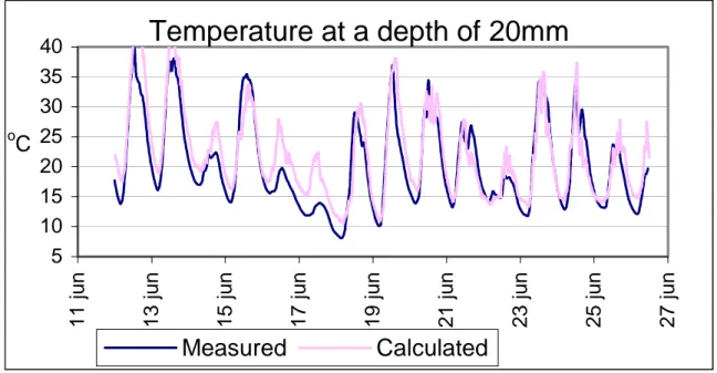
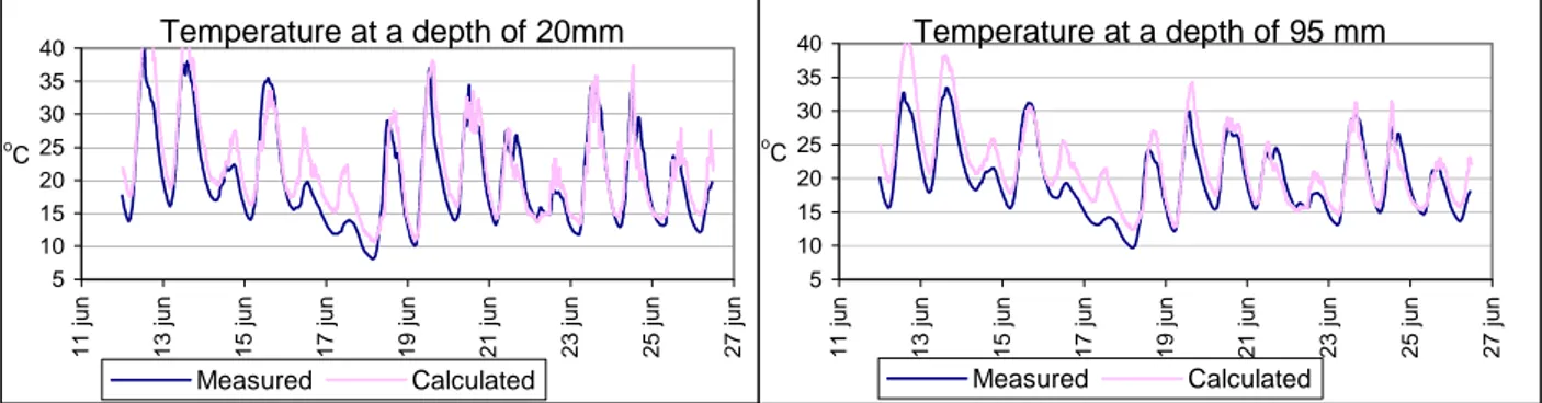
In Paper I a numerical model is described for the calculation of elevated temperatures in pavements during summertime. The model has been developed by the author and uses finite difference approximation of the heat conduction equation when calculating how heat is distributed in the pavement as a function of time. In the paper, a detailed description is also given of the sub-models for short-wave radiation, long-wave radiation and emission and convection losses, which are included in the numerical model. The model has been validated against measurements of temperatures on three different levels below the road surface in an asphalt concrete pavement on road, E18 outside the city Köping west of Stockholm, Sweden. In Figure 1, a comparison is shown for the calculated and measured temperatures at a depth of 20 mm below the rod surface. For the calculation of the pavement temperatures, input data have been obtained from The Swedish Meteorological and Hydrological Institute. Data regarding solar radiation are taken from Stockholm and air temperatures have been taken from a measuring station nearby the site where pavement temperatures where recorded.

Figure 1 Temperatures at a depth of 20 mm on Road E18 during the period June 12 to June 25, 1997. The diagram shows measured and calculated temperatures. Moreover, validation has also been made against measurements performed at a sunny summer day on a small road near the city Köping.

The model has also been used to calculate the highest possible temperature in asphalt concrete pavement. The position of the sun was calculated hour by hour and the sky was assumed to be completely cloudless. Further, the air temperature was set high in relation to the actual site, and it was supposed to be completely calm in order to achieve the highest possible temperature of the pavement. In Figure 2, calculated pavement temperatures are shown as function of time. In figure 2, the input air temperatures are given as the black solid line. The first six days, the input temperatures are those observed during a normal chilly summer day in mid Sweden. The following seven days are modeled as very warm days with completely clear sky, high air temperature and no wind. As has been mentioned previously, the highest pavement temperature is very essential when mixing the ingredients in asphalt in order to achieve a material with desired properties. In USA, the method given in SUPERPAVE serves

Temperature at a depth of 20mm

11 jun 13 jun 15 jun 17 jun 19 jun 21 jun 23 jun 25 jun 27 jun

o

C

3

as a tool for predicting, among other things, the highest temperature in the pavement based upon latitude and air temperature. This method is criticized in Paper I, as it implies the erroneous assumption that there is equilibrium when the highest temperature is reached.

Figure 2 Calculated surface temperatures as function of time. The black line shows the used input, air temperatures.

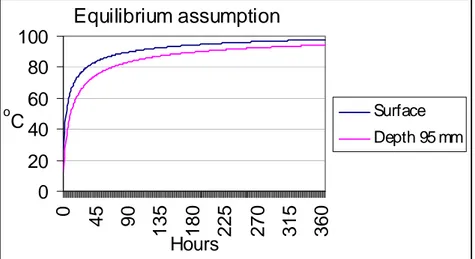
The consequence of this assumption is, that the highest temperature is heavily overestimated as the temperature is obtained with the assumption that the sun is constantly at its 12 o’clock position on Midsummer Day. The pavement temperatures obtained with this assumption are shown in Figure 3. Thus, a surface temperature near 100 oC should be obtained, which is approximately 30 oC higher than what is shown in Figure 2. However, this discrepancy is then compensated for in SUPERPAVE by assuming that the wind speed is 4.5 m/s, when the highest temperature is reached. However, it is the author’s opinion that it is much more probable that high temperatures are reached at feeble winds.

Figure 3 Calculated surface temperatures and the temperature at a depth of 95 mm obtained by the author’s model with the assumptions in SUPERPAVE. The air temperature is set to 30oC and it is also assumed to be completely calm.

Equilibrium assumption

0

20

40

60

80

C

3. LABORATORY FREEZING TESTS AND NUMERICAL FROST MODELING In Paper II a very simple model of how water is transported to the frozen parts of the soil structure and thus causing frost heave of the surface and water/ice accumulation within the soil mass is presented.

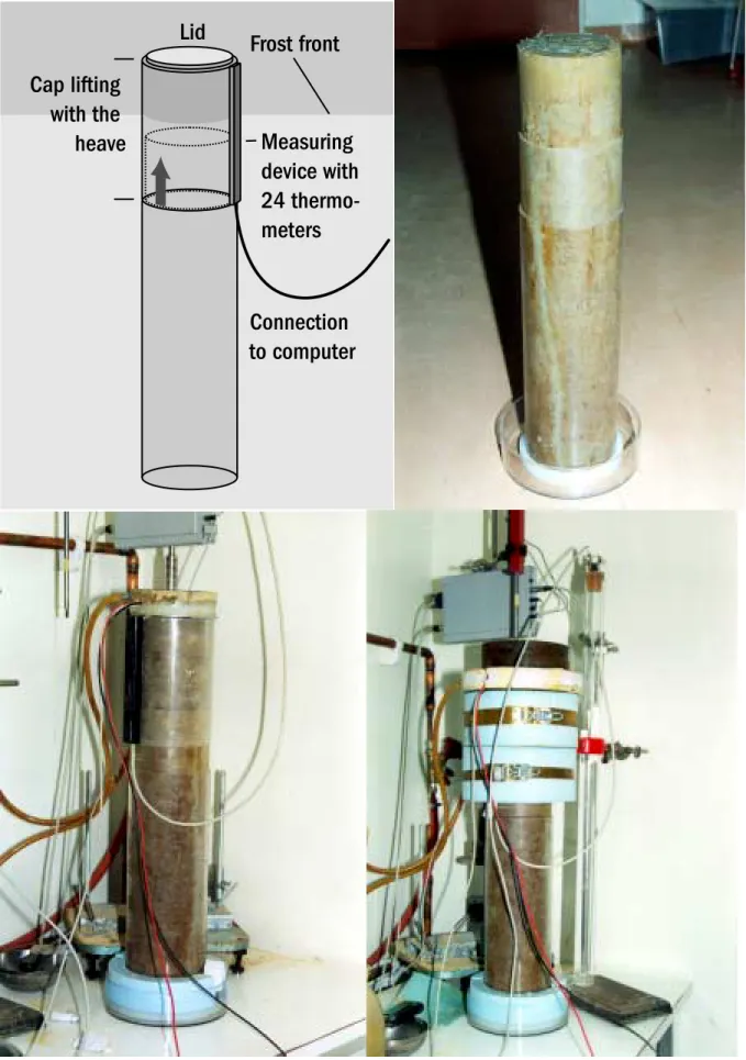
In paper II, it is also described a laboratory freezing testing device developed by the author during 1998. Freezing tests are normally performed on very small samples, typically being approximately 1 dm high, and for practical reasons they are in most cases cooled from bottom and up, and water is added from the top. This is in contrary to what applies in nature, where the cold comes from above and the supply of water is from below in the form of ground water. To study moisture transport in connection with freezing, an equipment was therefore constructed for samples somewhat more than 6 dm high, where cold and water are added from the ”right” direction, see Figure 5.

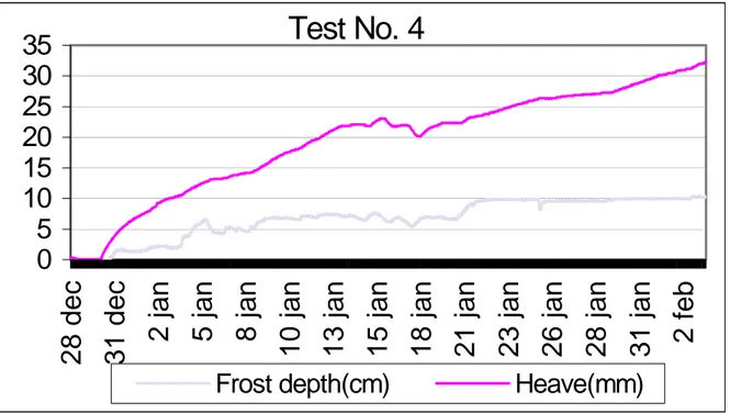
In paper II results are presented that frost heave can very well arise without the addition of external water, see Figure 4.

Figure 4. Frost depth and frost heave as function of time in a test performed without addition of external water.

Test No. 4

0

5

10

15

20

25

30

35

28 dec

31 dec

2 jan

5 jan

8 jan

10 jan

13 jan

15 jan

18 jan

21 jan

23 jan

26 jan

28 jan

31 jan

2 feb

5

Figure 5. The laboratory freezing equipment. It is shown how the tube is filled with a sample, fitted with the cap and then used in a test.

The natural existence of moisture (water content), in material susceptible to frost heave is shown to be quite sufficient for a considerable frost heave. This result contradicts with what normally is found in literature as the explanation to observed frost heave. It is in general assumed, that the heave directly corresponds to the amount of water taken up from the ground water, taking the 10 % volume expansion into consideration when water turns into ice. Results from a number of freezing tests with the equipment, designed by the author, are described in Paper II and it is especially commented how the heave rate seems to depend on the cooling rate of the sample. Results from field observations are also used to illustrate the dependence of the heave rate on the cooling rate (in this case the air temperature). The main part of Paper II contains a description of the numerical model, developed by the author, for the freezing of pavements. The model uses a finite difference approximation of the heat conduction equation in combination with a very simplified assumption of the relation between the cooling rate and the heave rate in order to describe the freezing process. In the model, the frost depth and the frost heave are continuously calculated. Temperature of the pavement surface and the material properties of the pavement are used as input data.

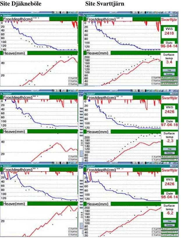
On two minor roads in Sweden, at Svarttjärn and Djäkneböle, manual measurements of frost heave, frost depth and ground water levels have been taken every winter since 1995-96. Both places are located in Sweden at approximately N 64o between the two cities Umeå and Skellefteå. The program has been run by using climatic data from the winters 95-96, 96-97 and 97-98. Figure 6 shows the result of the numerical model together with field measurements. Fairly good agreement is obtained for both sites during the three years. It is clear that the frost heave is completely different at the two sites, even though they are close enough to have an almost identical climate. Even though the frost heave behavior is very different at the two sites, the presented software enables to model the measured frost-heave behavior with acceptable accuracy.

7

Site Djäkneböle

Site Svarttjärn

Figure 6. Solid curves show calculated frost heave and frost depth. Field measurements are shown as dots. The left-hand diagram applies to the site Djäkneböle and the right-hand diagram to the site Svarttjärn. The uppermost diagrams are from winter 1995-96, followed by 1996-97 and 1997-98.

4. FROST HEAVE AND WATER UPTAKE DURING FREEZING TESTS

In Paper III, the relation between the frost heave and the amount of water sucked up by a sample during a freezing test in laboratory is discussed. Many researchers assume that the heave is 10 % greater than the water intake, as water expands by 10 % when it freezes. It is then presumed that the sample is initially saturated and that the unfrozen part remains saturated in the course of the test. In Paper III, papers by three established researchers - Loch (1979), Penner (1960), and Konrad (1984) - assuming that the heave is 1.1 times the water intake are discussed. One of these, Loch, shows measurements of both heave and water intake from ten different freezing tests. In two of these tests the heave is essentially (more than 10 %) greater than the water intake during the first days, which the author of the paper has apparently not observed, since the contrary is claimed in the paper.

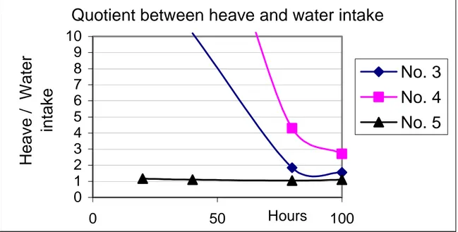
In Figure 7, data read from diagrams in the paper by Loch are used to show that the heave can be considerably greater than the water intake. In Figure 7 the quotients between the heave and water intake are shown, all read from Figures 2 and 3 in the paper by Loch. It should be noticed, that for sample No. 5, the quotient between the heave and water intake is approximately 1.1 during the whole course of the test. For the other samples, however, the heave is considerably greater than the water intake. Although the tests have proceeded for four days the heave is in one case three times greater than the water intake.

Figure 7. The diagram shows the quotient between heave and water intake according to data from Loch (1979).

In Paper III, results from freezing test performed by the author is again shown, highlighting a strong heave without any addition of external water whatsoever, see Figure 4. The explanation presented in Paper III of this behavior, i.e. a heave being obtained without any addition of external water, is based upon the following hypothesis. The material in the unfrozen part of the sample i.e. below the freezing front is being partly dried out and thus supplying the freezing front with water to the created ice lenses. The assumption is then, that ice lenses being located outside the pores demand space, which causes a heave, whereas the water used,

Quotient between heave and water intake

0

1

2

3

4

5

6

7

8

9

10

0

50

Hours

100

Heave / W

a

ter

intake

No. 3

No. 4

No. 5

9

was located in pores further down in the sample. These pores are supposed to have mainly the same size as before they were partly drained out, and thus mainly the same size as before the freezing test started. This means that the water, which gives an increased volume in the form of ice, is taken from the underlying layer without a corresponding decrease in volume. The result is then a net increase of the volume without the addition of external water.

5. REFERENCES

Barber, E. S. (1957) Calculation of Maximum Pavement Temperatures from Weather Reports. Bulletin 168, HRB, National Research Council, Washington, D.C., pp. 1-8

Beskow, G. (1935). Soil freezing and frost heaving with special application to roads and railroads. The Swedish Geological Society, C, no. 375, Year Book no. 3.(In Swedish) Bjurulf, A, & Nordmark, U. (1994). Vägstandardens inverkan på skogsindustrins

råvara.(Standard of roads and the influence on supply of raw materials to the forest industry) In Swedish with Summary in English. The Forestry Research Institute of Sweden, SKOGFORSK

Geiger, R. (1959) The Climate Near the Ground. Harvard University Press, Cambridge, Mass. Gustafson, K. (1981) Road icing on different pavement structures. Swedish National Road

and Transport Research Institute, VTI Rapport 216A

Henry, K. S. (1998). The Use of Geosynthetics to Mitigate Frost Heave in Soils.Ph.D. University of Washington.

Johansen, O. (1975). Thermal conductivity of soils. Ph.D. Trondheim. The Norwegian Institute of Technology.

Kaplar, C.W. (1970). Phenomenon and Mechanism of Frost Heaving. Highway Research Record 304, pp. 1 - 13.

Knutsson, S. (1998). Soil Behavior at Freezing and Thawing. Thesis 1998:20, Luleå University of Technology.

Konrad, J.-M. (1984). Soil freezing characteristics versus heat extraction rate. National Research Council of Canada, DBR Paper No 1257, Ottawa, Ontario.

Konrad, J.-M. (1987). Procedure for Determining the Segregation Potential of Freezing Soils. Geotechnical Testing Journal, GTJODJ, Vol. 10, No. 2, June 1987, pp. 51-58.

Kreith, F. (1973) Principles of Heat Transfer, 3 rd ed. Harper and Row Publishers, New York Loch, J. P. G. (1979). Influence of the Heat Extraction Rate on the Ice Segregation Rate of

Soils. Frost i jord, No 20, pp. 19 - 30.

Penner, E. (1960). The Importance of Freezing Rate in Frost Action in Soils. Proc. ASTM, Vol. 60, pp. 1151-1165.

Penner, E (1972). Influence of Freezing Rate on Frost Heaving. Highway Research Record, No 393 , pp. 1 – 11.

Rumney, T. N., and R. A. Jimenez. (1969) Pavement Temperatures in the Southwest. In Highway Research Record 361, HRB, National Research Council, Washington, D.C., pp. 1-13

Sellers, W. D. (1972) Physical Climatology. University of Chicago Press. Chicago & London. Solaimanian, M., and T. W. Kennedy. (1993) Predicting Maximum Pavement Surface

Temperature Using Maximum Air Temperature and Hourly Solar Radiation. In Transportation Research Record 1417, pp. 1-11.

Stenberg, L (1979). Full scale frost heave tests. Uppsala: Kvartärgeologiska fören.

Sundberg, J.(1988) Thermal Properties of Soils and Rocks. SGI Report No. 35, Linköping Superpave: Performance Graded Asphalt Binder Specification and Testing. Asphalt Institute.

Paper I

A Simulation Model for the Calculation of Pavement

Temperatures, Including the Maximum Temperature.

Åke Hermansson

Presented at the Transportation Research Board (TRB) Annual Meeting,

Washington DC, USA, January 9 – 13, 2000.

A Simulation Model for Calculating Pavement Temperatures, Including the

Maximum Temperature

Åke Hermansson. Researcher, Highway Engineering, Swedish National Road and Transport Research Institute, VTI, SE-581 95 Linköping, Sweden and Dept. of Civil and Mining Eng. at Luleå University of Technology.

Åke Hermansson VTI SE-581 95 Linköping Sweden Phone: +4613204072 Fax: +4613141436 Email: ake.hermansson@vti.se

2 ABSTRACT

A simulation model has been developed to calculate the temperatures of the asphalt concrete during summer. Input data to the simulation model are hourly values for solar radiation, air temperature and wind velocity. Longwave radiation incident to and outgoing from the

pavement surface is calculated from the air and pavement surface temperatures, respectively. The portion of the incident shortwave radiation absorbed by the pavement surface is

calculated from the albedo of the surface. By means of a finite difference approximation of the heat transfer equation, the temperatures are calculated under the surface. Apart from radiation and heat transfer, convection losses from the pavement surface are also calculated depending on wind velocity, air temperature and surface temperature.

The formulas used for the calculation of radiation and the simulation model as a whole are validated by comparison with measurements, showing good agreement.

A method for the calculation of direct solar radiation from a clear sky, at an arbitrary location and time, is used to create input data to the simulation model in order to calculate maximum pavement temperatures.

The formulas used in “Superpave” to calculate maximum pavement temperatures are based on the assumption that there is an equilibrium when a maximum temperature is reached. Such an equilibrium assumption can strongly be questioned, and its consequences are discussed in the paper. Key words: Pavement temperatures Maximum temperature Simulation model Superpave

1 Introduction

The asphalt concrete in pavements is exposed to great strains and stresses. Above all, heavy vehicles put forward strong demands for pavement properties. The traffic affects the asphalt concrete in different ways during summer and winter. During winter it is relatively hard and cracks can arise as frost cracking or as temperature cracks when the pavement shrinks longitudinally. During the summer it is softer, and during strong sunshine on hot days, the risk is high that heavy vehicles cause rutting due to plastic deformation. The various substances of the asphalt concrete and their proportioning can modify its properties.

Consideration should thereby be taken to the lowest and highest expectable temperatures of the asphalt concrete. These temperatures of course differ dependent on the weather conditions existing at different locations. In the USA, a binder and mixture specification for pavement design called Superpave (7) was developed under the Strategic Highway Research Program (SHRP). Superpave is supposed to be able to be applied over the whole continent for paving measures. Besides traffic parameters, the lowest and highest pavement temperatures are included there.

Theories for longwave radiation and shortwave radiation in the atmosphere and the

interaction of the radiation with the earth surface have been thoroughly treated by a number of authors, Kreith (4), Sellers (5), Geiger (2) and others. Barber (1) was one of the first to

develop a specific model for the calculation of pavement temperatures. He suggested a thermal diffusion theory, using daily radiation and its effect on the mean effective air temperature. Rumney and Jimenez (8) developed a method using empirical nomograhs to predict pavement temperatures at a depth of 2 in. These graphs were based on pavement temperature measurements in combination with hourly measurements of air temperature and solar radiation. The simulation model proposed in this paper is built on formulas for

convection, shortwave and longwave radiation as described by Solaimanian and Kennedy (6). It also contains a finite difference approximation for the calculation of heat transfer down into the pavement and underlying sub-grade. Input data to the model are hourly values for solar radiation, air temperature and wind velocity. For the heat transfer calculation, the porosity and the degree of water saturation of the different layers are also needed.

When validating the simulation model by comparing the output with measured pavement temperatures, measured values are used as climate data. For the calculation of maximum pavement temperatures a method for computing direct solar radiation, described by

Solaimanian and Kennedy, is used. It gives the direct solar radiation from a clear sky at an optional time and location, and is used to create climate data, when calculating maximum pavement temperatures in the simulation model. In Superpave, the formula described by Solaimanian and Kennedy is used when calculating maximum temperatures. The formula is built on an equilibrium assumption. The results obtained under such an assumption are compared with the output from the simulation.

4 2 Theory

2.1 Radiation balance

2.1.1 Outgoing longwave radiation

The earth surface is assumed to emit longwave radiation as a black body. Thus, the outgoing longwave radiation follows Stefan-Boltzman law, Solaimanian and Kennedy, Kreith, Sellers and Gustafson (3).

4

s

r T

q =εσ (1)

where q_r is the outgoing radiation in W/ m2, ε emission coefficient, σ is Stefan-Boltzman constant 5.68∗10−8W/(m2K4)and T_sis the temperature of the surface in oK. 2.1.2 Longwave counter radiation

The atmosphere absorbs radiation and emits it as longwave radiation to the earth, so-called counter radiation. Counter radiation absorbed by the pavement surface can be calculated as, Solaimanian and Kennedy

4

air a

a T

q =ε σ (2)

where q_ais absorbed counter radiation in W/ m2,ε_a can be set to 0.7 on a clear day and air

T is the air temperature in oK. 2.1.3 Shortwave radiation

The surface of the sun has a very high temperature, approx. 6000 oK, and therefore emits radiation of high frequency (shortwave). Part of this radiation is diffusely scattered in the atmosphere of the earth in all directions and the diffused radiation reaching the earth is called diffuse incident radiation. Radiation from the sun reaching the earth surface without being reflected by clouds, absorbed or scattered by the atmosphere is called direct shortwave radiation. The distribution of direct and diffuse radiation is dependent on the weather. Clear weather causes a larger portion of direct radiation.

2.2 Convection

The convection losses can be calculated as, Solaimanian and Kennedy )

( _{s air} c

c h T T

q = − (3)

where qc is the loss to the air in

2

/ m

W . The parameter hc depends on the surface temperature and essentially the wind velocity

] ) ( 00097 . 0 00144 . 0 [ 24 . 698 m0.3 0.7 s air 0.3 c T U T T h = + −

where U is the wind velocity in m/s and T_mis the average value of the surface and air temperature in oK.

2.3 Heat transfer

The above describes the energy absorbed and emitted by the pavement surface. Heat is also exchanged with the ground under the surface through heat transfer. This can be handled with e.g. finite difference approximations of the heat transfer equation.

3 Validation of components in the radiation balance

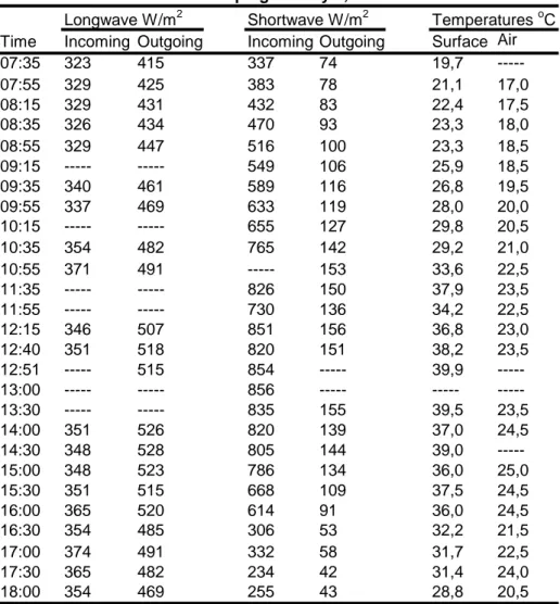
On July 9, 1998 radiation measurements were made on a small road near Köping, 100 km west of Stockholm. The pavement surface was rather light. The measurements went on from 7:35 a.m. until 6 p.m. and were registered two or three times per hour. The weather was extremely sunny the whole morning, not once did clouds or haze block out the sun. The fine weather continued in the afternoon, however with some slight cloudiness during early afternoon and later with rather dense clouds. Longwave as well as shortwave radiation were measured, both outgoing from the pavement surface and incident to the surface. Moreover, air and pavement surface temperatures were measured, see Table 1. These measurements are used below to validate the formulas for the calculation of the components forming part of the radiation balance.

3.1 Calculation of incoming longwave radiation

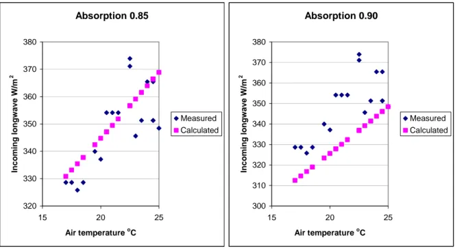
Incoming longwave radiation absorbed by the pavement surface is given by Formula 2. As the absorption coefficient ε gives the portion of the incident radiation absorbed by the surface, the calculated absorbed incident radiation must be divided by ε to obtain the corresponding incident radiation. Below, calculated and measured incident radiation for ε = 0.85 and ε = 0.90 is shown, see Figure 1. Consequently, the graphs show the dependence of the incident longwave radiation on the air temperature.

6 3.2 Calculation of outgoing longwave radiation

Longwave outgoing radiation from the pavement surface is given by Formula 1. As the radiation measured also includes the reflected part of the incident radiation, the outgoing radiation is calculated as q_r+ the part (1 - ε) of the measured incident radiation. Below, calculated and measured outgoing radiation is shown for ε = 0.85 and ε = 0.90, see Figure 2. Consequently, the graphs show the dependence of the outgoing longwave radiation on the pavement surface temperature.

The incident radiation gives the best agreement for the absorption coefficient ε = 0.85. The outgoing radiation agrees approximately equally well for the emission coefficientε = 0.85 and 0.90. As the emission coefficient and the absorption coefficient are in reality the same, it is set equal to 0.85.

TABLE 1 Measurements at Köping on July 9, 1998.

Longwave W/m2 Shortwave W/m2 Temperatures oC

Time Incoming Outgoing Incoming Outgoing Surface Air

07:35 323 415 337 74 19,7 ---07:55 329 425 383 78 21,1 17,0 08:15 329 431 432 83 22,4 17,5 08:35 326 434 470 93 23,3 18,0 08:55 329 447 516 100 23,3 18,5 09:15 --- --- 549 106 25,9 18,5 09:35 340 461 589 116 26,8 19,5 09:55 337 469 633 119 28,0 20,0 10:15 --- --- 655 127 29,8 20,5 10:35 354 482 765 142 29,2 21,0 10:55 371 491 --- 153 33,6 22,5 11:35 --- --- 826 150 37,9 23,5 11:55 --- --- 730 136 34,2 22,5 12:15 346 507 851 156 36,8 23,0 12:40 351 518 820 151 38,2 23,5 12:51 --- 515 854 --- 39,9 ---13:00 --- --- 856 --- --- ---13:30 --- --- 835 155 39,5 23,5 14:00 351 526 820 139 37,0 24,5 14:30 348 528 805 144 39,0 ---15:00 348 523 786 134 36,0 25,0 15:30 351 515 668 109 37,5 24,5 16:00 365 520 614 91 36,0 24,5 16:30 354 485 306 53 32,2 21,5 17:00 374 491 332 58 31,7 22,5 17:30 365 482 234 42 31,4 24,0 18:00 354 469 255 43 28,8 20,5

Figure 1 Calculated and measured incoming longwave radiation at different air temperatures.

Figure 2 Calculated and measured outgoing longwave radiation as a function of

pavement surface temperature.

Absorption 0.85 320 330 340 350 360 370 380 15 20 25 Air temperature oC Incoming longwave W /m 2 Measured Calculated Absorption 0.90 300 310 320 330 340 350 360 370 380 15 20 25 Air temperature oC Incoming longwave W /m 2 Measured Calculated Emission 0.85 400 420 440 460 480 500 520 540 15 25 35 45 Surface temperature oC Outgoing longwave W /m 2 Measured Calculated Emission 0.90 400 420 440 460 480 500 520 540 15 25 35 45 Surface temperature oC Outgoing longwave W /m 2 Measured Calculated

8 3.3 Albedo for incident shortwave radiation

On July 10, 1998 measurements were performed of outgoing and incident shortwave radiation normal to the pavement surface on a test section on Road E18 at Köping, see Table 2. Albedo is defined as the part of the shortwave radiation reflected by the pavement surface and can thus be estimated as the measured outgoing radiation divided by the measured incident radiation. The measurements were made on a location where pavement temperature was measured during 1997, see Section 6.1. On account of heavy traffic, only three

measurements were made of albedo in close succession. However, the variation between the three measurements was small and the value 0.15 was selected as input to the simulation model.

4 The simulation model

The simulation model uses climate data in the form of hourly values for incident shortwave radiation, air temperature and wind velocity. The shortwave radiation is divided into diffuse and direct radiation normal to the horizontal plane. The radiation data to the climate file can be created either from measurements according to Section 5, or through calculation of maximum solar radiation according to Section 7.

During the simulation, the direct and the diffuse parts are not separated, but the same portion of both is absorbed. The portion reflected is equal to the albedo of the pavement surface. Longwave radiation is calculated by Formulas 1 and 2, and convection losses by Formula 3.

For the calculation of heat transfer, the ground is divided into cells, thin ones near the surface and thick ones at a deeper level. Each cell is assigned the properties temperature, porosity and degree of water saturation, of which only the temperature varies during the simulation. Thermal conductivity and thermal capacity are calculated using parameters of water, the material and air, Sundberg (9)

Each cell being given a temperature starts the calculation. The model then calculates a new temperature for each cell - several times for each simulated hour. This is done in accordance with a generally accepted heat transfer theory, i.e. heat flows from warmer to colder cells in an extension depending on temperature difference and thermal conductivity. The temperature change depends in its turn on the amount of energy received and the thermal capacity of the cell.

During the calculations, the exchange of energy of the uppermost cell through the pavement surface in the form of radiation and convection is also handled.

The cell division is made down to a depth of five meters where the temperature is supposed to be constant.

TABLE 2 Measurements of shortwave radiation on Road E18, July 10, 1998

Shortwave radiation W/m2

Time Incoming Outgoing Albedo

12:01 306 47 0,154

12:04 286 44 0,155

5 Input data to simulation

The climate file contains hourly values for diffuse incident shortwave radiation, direct incident shortwave radiation, air temperature and wind velocity. The Swedish Meteorological and Hydrological Institute (SMHI) measures shortwave radiation outside Stockholm, 100 km straight east of the test section at Köping, i.e. at the same latitude. The direct radiation is measured normal to the direction of the solar radiation. Since the simulation model presumes that the climate file contains the radiation normal to the pavement surface, the radiation measured must be converted. According to Solaimanian and Kennedy the zenith angle z for an arbitrary location for an optional date and time of the day is given by

φ δ

δ

φsin cos cos cos sin

cosz= s + s H (4)

H in Formula 4 is calculated as the angle remaining for the earth to rotate until the location in question has the sun as its highest on the sky the actual day. If, for example, 4 hours remain until noon (12.00), H is calculated as 4/24*360. In the afternoon the time passed since 12.00 is instead used. Thus, H is symmetrical round 12.00. δ_s expresses how the inclination of the axis of the earth changes with the time of the year. It varies in the interval +23.5 to - 23.5 degrees. During simulation, the simplification has been made that the inclination changes with the same amount each day during the whole year. On days 91 and 274 the inclination is approx. 0, whereas on day 0 is -23.5 and on day 182 +23.5. φ is the latitude of the location in question.

The radiation measured normal to the direction of the solar radiation is multiplied by

z

cos to obtain the radiation normal to the horizontal plane. To this direct radiation, the measured diffuse radiation is added. This yields the total shortwave radiation received at the pavement surface. 85% of this is supposed to be absorbed by the pavement surface, according to measurements of albedo on Road E18, see Table 2.

6 Validation of measurements and the proposed simulation model 6.1 Validation of the simulation model using data from Road E18

During the summer of 1997 the asphalt concrete temperature was measured at the levels 2 cm, 5 cm and 9.5 cm, under the surface. The temperatures were registered twice an hour during the whole summer. The measurements were made on Road E18 quite south west of the city of Köping and these data have been used for the validation of the simulation model. In the climate file there should be hourly values for diffuse shortwave radiation, direct shortwave radiation normal to the pavement surface, air temperature and wind velocity. The SMHI’s measurements from Stockholm, 100 km straight east of Köping, i.e. at the same latitude, contain these radiation values. However, the direct radiation is measured normal to the direction of the solar radiation and must be converted according to Formula 4. For air temperatures, the nearest road weather station was used.

The parameter ε_a was set equal to 0.7 for calculating longwave counter radiation, ε the emission coefficient for calculating outgoing longwave radiation was set equal to 0.85 according to Section 3.2, and the absorption of shortwave radiation was set equal to 0.85 according to measurements of albedo on Road E18, see Table 2. The parameter h for _c

calculating convection losses was set corresponding to a wind velocity of 4.5 m/s (the value used by Solaimanian and Kennedy). With these climate data and values for parameters, the

10

simulation yielded pavement temperatures which were the whole time lower than the ones measured. The only parameter not verified with measurements was h (unfortunately there c were no wind data available from the test section for the summer of 1997).

Trial and error showed that h corresponding to a wind velocity of 1 m/s yielded a good _c

agreement between measurement and calculation. Below, calculated and measured

temperatures are shown at two different depths of the pavement, Figure 3. On June 16 and 17 there was evidently not very much sunshine and on these days the worst agreement was obtained. This could be explained by ε_a having been selected at 0.7 and this is supposed to correspond to a clear sky. When it is cloudy this probably implies an underestimation of the counter radiation.

Figure 3 Temperature at a depth of 20 mm, and 95 mm respectively, on Road E18 at

Köping during the period June 12 to June 25, 1997. The diagrams show measured and calculated temperatures.

6.2 Validation of measurements at Köping

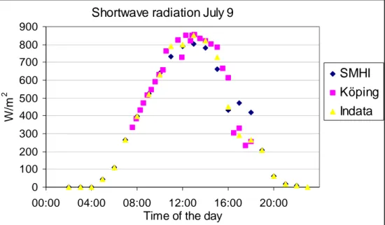
As has already been mentioned, the SMHI performs measurements of direct and diffuse shortwave radiation, in Stockholm. In Figure 4 the SMHI’s measurements from Stockholm, July 1997 are shown. High direct radiation and comparatively low diffuse radiation

characterise clear days. Apparently, July 9, 1997 happened to be a clear day similar to July 9, 1998 when the measurements at Köping, shown in Table 1, were performed. Stockholm and Köping are at the same latitude 100 km distant from each other.

The 1998 measurements at Köping correspond to a radiation normal to the pavement surface, whereas the SMHI measures normal to the direction of the solar radiation. To enable these measurements to be compared, the SMHI measurements must be converted to normal to the pavement surface. This is achieved by multiplying by cos z, calculated according to Formula 4.

In Figure 5 the total of direct and diffuse incident shortwave radiation is shown. The diagram shows the Köping measurements from July 9, 1998 and the SMHI’s measurements from July 9, 1997.

The measurements in Figure 5 show a good agreement, which verifies both the 1998 measuring method and the formula to convert the SMHI’s measurements to normal to the pavement surface. Temperature at a depth of 20mm 5 10 15 20 25 30 35 40

11 jun 13 jun 15 jun 17 jun 19 jun 21 jun 23 jun 25 jun 27 jun

o C Measured Calculated Temperature at a depth of 95 mm 5 10 15 20 25 30 35 40

11 jun 13 jun 15 jun 17 jun 19 jun 21 jun 23 jun 25 jun 27 jun

o C

Figure 4 Direct and diffuse radiation during July, 1997 according to the SMHI’s measurements.

Figure 5 Total shortwave radiation according to measurements on July 9, 1998 and

the SMHI’s measurements on July 9, 1997. The diagram also shows the values used for simulation, Köping, July 9, 1998.

Shortwave radiation.

1 jul 2 jul 4 jul 6 jul 8 jul

10 jul 12 jul 14 jul 16 jul 17 jul 19 jul 21 jul 23 jul 25 jul 27 jul 29 jul 31 jul

W/m

2

Direct Diffuse

Shortwave radiation July 9

0 100 200 300 400 500 600 700 800 900 00:00 04:00 08:00 12:00 16:00 20:00

Time of the day

W/ m 2 SMHI Köping Indata

12

6.3 Validation of the simulation model using data from Köping

In Section 6.1 the SMHI’s measuring values of solar radiation during June, 1997 were used as input data to the simulation model to compare calculated and measured temperatures at different levels in the pavement.

On July 9, 1998 measurements were made of air temperature, shortwave radiation and the pavement surface temperature close to the test section on Road E18 at Köping, see Table 1. These data have also been used to validate the simulation model by comparing measured surface temperatures with those calculated by the model. Input data necessary for this purpose are hourly values for shortwave radiation received at the pavement surface and the air

temperature. Moreover, the wind velocity has to be known to enable the setting of the parameter h when calculating convection losses. The measurements of radiation were made _c

momentaneously without any great regularity, see Table 1, and can therefore not be used as hourly values. Nor did the measurements comprise all the time the sun was out. To obtain hourly values for incident shortwave radiation, the measurements were used for the time they were available and the SMHI’s Stockholm values from July 9, 1997 for morning and evening. Figure 5, which contains both the measurements from July 9, 1998 and the SMHI’s

measurements from July 1997, was used to estimate hourly values. Hourly values were entered into the diagram manually, Figure 5, so that it looked reasonable compared to the 1998 measurements and so that they totally corresponded to those of the SMHI in the morning and evening. The symbol ‘input data’ in the diagram shows the hourly values selected as input data to the simulation.

The 1998 Köping measurements were used as air temperatures for the time they were available. For other times the SMHI’s measurements from Sala were used, being the nearest measuring station. These were registered every third hour and interpolated to hourly values. For the convection it is also necessary that the wind velocity is known. The wind in Sala increased from 2 m/s to 4 m/s during the day. At Köping the wind was felt as rather strong and approximately equally strong the whole day. In view of this, h was set equal to 17, which c corresponds to 4 m/s. In this way h was determined and there were hourly values for air c temperatures and incident shortwave radiation covering a whole day. To give the simulation the possibility of oscillating in, the weather corresponding to July 9 were repeated a number of times in the input data file. Thus, the simulation repeated the July 9 data a couple of times until the calculated temperature course was the same. In Figure 6 calculated and measured surface temperatures for July 9, 1998 at Köping are shown. The morning was completely cloudless but in the afternoon it became cloudier and clouds were blocking the sun now and then. Between the clouds it was completely clear, however. It was difficult to measure incident radiation when the clouds were passing. The instruments were extremely sensitive and quick and drifted considerably when clouds were passing. One of the purposes of the measurements was to estimate albedo, which demands simultaneous and stable values for both incident and outgoing radiation. This implied that the measuring values were often taken during clear periods, which may have caused an overestimation of the radiation in the early afternoon. This could be an explanation to why calculated surface temperatures are too high at the beginning of the afternoon.

Figure 6 The pavement surface temperature at Köping on July 9, 1998. The diagram shows measured and estimated temperatures.

7 Calculation of maximum pavement temperatures 7.1 Calculation of maximum direct solar radiation

According to Solaimanian and Kennedy the direct solar radiation normal to the direction of the solar radiation can be calculated as

m n

R =1394⋅τ_α (5)

Where τ_α varies between 0.62 and 0.81 depending on the weather. 0.81 is supposed to correspond to clear weather. The parameter m is calculated as 1/cosz where cos is z

obtained from Formula 4. In Figure 7 the direct radiation in accordance with this calculation is shown, for τ_α = 0.81, andτ_α = 0.75. As a comparison there are also the SMHI’s measuring values from July 9, 1997. All values have been multiplied by cos to be valid for a horizontal z

surface.

This method is used in Section 7.2 in order to calculate maximum pavement temperatures during an imagined longer period with completely clear weather.

Surface temperature at Köping July 9 1998

0 5 10 15 20 25 30 35 40 45 00: 00 02: 00 04: 00 06: 00 08: 00 10: 00 12: 00 14: 00 16: 00 18: 00 20: 00 22: 00

Time of the day

o

C Computed

14

Figure 7 Calculated direct shortwave radiation for τ_α = 0.81 and τ_α = 0.75. The

diagram also shows the SMHI’s measurement on July 9, 1997.

7.2 Maximum pavement temperatures according to the proposed simulation model By combining Formulas 4 and 5 the direct shortwave radiation normal to the pavement surface can be calculated for an arbitrary location for an optional day and hour. Thus, an imagined maximum direct radiation on a Midsummer Day at Köping has been calculated, hour by hour, with τ_α = 0.81. As hourly values for diffuse radiation the SMHI’s values from July 9, 1997 were used, which can represent a clear summer day. The air temperature was simply set equal to 30oC when the sun is out and 20oC at night. These values of direct and diffuse shortwave radiation and air temperatures, respectively, were selected to represent the weather, which is supposed to give maximum pavement temperatures.

An input file was created starting by some normal cool days. After that, the ‘max day’ was repeated several times in the input file.

In Figure 8 the surface and air temperatures are shown from two different runs with different values of the h , i.e. different wind velocities. One can see that the maximum _c

surface temperature is very much dependent on the wind velocity. Moreover, it appears that the number of days with maximum weather have a much greater importance when the winds are weak. Then, the day max continues to increase considerably during several days, which is not at all the case with somewhat stronger winds.

Direct radiation July 9 1998

0 200 400 600 800 1000 1 3 5 7 9 11 13 15 17

Time of the day

W/m

2 _{Talf .81}

SMHI Talf .75

Figure 8 Surface temperature calculated with the simulation model. The input file is opened with some normal chilly days, from measurements, followed by days with a high air temperature and maximum solar radiation.

7.3 Maximum pavement temperatures according to Superpave

In Superpave there are binder and mixture specifications calculated from the highest and lowest pavement temperatures expectable at different locations in the USA. The formula on page 50 in Superpave is to be used to calculate the high pavement design temperature at a depth of 20 mm in the pavement according to

78 . 17 ) 9545 . 0 )( 2 . 42 2289 . 0 00618 . 0 ( 2 20 = T − Lat + Lat+ − T mm air (6) where mm

T₂₀ is the high pavement design temperature at a depth of 20 mm air

T is the average air temperature for the hottest seven-day period on the location Lat is the latitude of the location

The formula above is calculated by means of the following equation, Equation (12) in Solaimanian and Kennedy

0 ) ( ) ( cos

1394 1/cosz + _{a air}4 − _{c s}− _air − T_s−T_d − T_s4 =

d k T T h T z ε σ εσ ατα (7) where

α = absorption coefficient for shortwave radiation

k = the heat transfer coefficient for the ground

d

T = the temperature at the depth d

The first term of the equation corresponds to the maximum direct shortwave radiation, see Formula 5. The second term is longwave counter radiation, see Formula 2, the third is

convection losses to the air, see Formula 3, the fourth is heat transfer down into the ground and the fifth term corresponds to outgoing longwave radiation, see Formula 1. There is no term for diffuse shortwave radiation. Behind the equation lies an assumption about

Air and surface temperatures, when calm

0 10 20 30 40 50 60 70 80 13 j u n 14 j u n 15 j u n 17 j u n 18 j u n 19 j u n 21 j u n 22 j u n 23 j u n 24 j u n o C

Air and surface temperatures, wind 4m/s

0 10 20 30 40 50 60 70 80

13 jun 13 jun 14 jun 15 jun 16 jun 17 jun 18 jun 19 jun 20 jun 21 jun 22 jun 23 jun

Air Surface

16

equilibrium, i.e. that the total of the five terms is equal to zero when the pavement surface reaches its maximum temperature. There is no term corresponding to the fact that the surface layer consumes energy when its temperature increases, but, as has been stated previously, it is assumed that the surface has reached the equilibrium temperature corresponding to the five terms. Thus, in Equation 7 the surface temperature is sought which would be reached after a very long time with a constant high air temperature and a constant maximum solar radiation. This assumption must be questioned, as we know that the temperature of the pavement surface changes very quickly on sunny days when high temperatures are reached. When the maximum surface temperature is reached, usually round 2 p.m., the surface temperature is far from the equilibrium temperature.

The Superpave method is based on the assumption that the equilibrium is reached when the sun is at its highest at 12 o’clock on Midsummer Day, at the same time as the air is very warm. In the simulation, such an assumption is equivalent to freezing the sun at its noon position on Midsummer Day and simultaneously keeping a high air temperature constant during a long time.

The pavement temperature obtained under such an assumption is the temperature reached asymptotically in Figure 9. Thus, a surface temperature near 100oC is obtained, which is approx. 30oC higher than shown in Figure 8. When calculating the maximum temperature in Superpave, a wind velocity of 4.5 m/s is used for a reason not verified. This must be

questioned, as it is more likely for high temperatures to occur when convection losses are low. Figure 8 show that the wind velocity of 4 m/s reduces the surface temperature by approx. 25oC compared with calm. The two assumptions, equilibrium at a maximum temperature and that a maximum temperature is achieved at 4.5 m/s, on the whole cancel each other out.

Figure 9 Surface temperature and the temperature at a depth of 95 mm calculated

with the simulation model. The sun is kept in its highest position on Midsummer Day.

The air temperature is 30oC and it is completely calm.

Equilibrium assumption 0 20 40 60 80 100 0 45 90 135 180 225 270 315 360 Hours o C Surface Depth 95 mm

8 Conclusions

The proposed simulation model can, according to comparisons with field measurements, calculate the temperatures of the pavement at different levels during summer days. The simulation model does not consider rainfall and is most suitable for fine weather. The

formulas included in the simulation for the calculation of longwave radiation to and from the pavement surface agree well with measured values. The simulation model can also be used to calculate the maximum pavement temperatures at different latitudes.

In Superpave it is assumed there is an equilibrium when a maximum temperature is reached. This equilibrium assumption increases, under certain circumstances, the calculated maximum surface temperature by approx. 30oC. Furthermore it is shown that when assuming, as in Superpave, that a maximum temperature is reached at a wind velocity of 4.5 m/s the temperature is underestimated by approx. 25oC, compared to what is reached during calm. The two assumptions, equilibrium at a maximum temperature and that a maximum

temperature is achieved at 4.5 m/s, on the whole cancel each other out and the final result agrees in certain cases with the one obtained from the simulation.

References

6. Barber, E. S. Calculation of Maximum Pavement Temperatures from Weather Reports. Bulletin 168,

HRB, National Research Council, Washington, D.C., 1957, pp. 1-8

7. Geiger, R. The Climate Near the Ground. Harvard University Press, Cambridge, Mass., 1959.

8. Gustafson, K. Road icing on different pavement structures. Swedish National Road and Transport

Research Institute, VTI Rapport 216A, 1981

9. Kreith, F. Principles of Heat Transfer, 3 rd ed. Harper and Row Publishers, New York, 1973.

10. Sellers, W. D. Physical Climatology. University of Chicago Press. Chicago & London, 1972.

11. Solaimanian, M., and T. W. Kennedy. Predicting Maximum Pavement Surface Temperature Using

Maximum Air Temperature and Hourly Solar Radiation. In Transportation Research Record 1417, 1993, pp. 1-11.

12. Superpave: Performance Graded Asphalt Binder Specification and Testing. Asphalt Institute. Superpave

Series No. 1 (SP-1).

13. Rumney, T. N., and R. A. Jimenez. Pavement Temperatures in the Southwest. In Highway Research

Record 361, HRB, National Research Council, Washington, D.C., 1969, pp. 1-13

Paper II

A New Simple Frost Model, Validated and Easy to Use

Åke Hermansson

Proc. Tenth International Conference on Cold Regions Engineering, Lincoln New Hampshire USA, August 16 - 19, 1999, (Ed.: Jon E. Zufelt), ASCE, Reston Virginia USA, pp. 199 - 210

A New Simple Frost Model, Validated and Easy to Use

Abstract

New equipment for performing freezing tests on soil materials is developed in order to study water transport during the freezing cycle. Laboratory freezing tests and field measurements indicate that the heave rate is almost independent of the heat extraction rate when freezing is in progress. These findings are built into a simulation program, which is presented.

1 Introduction

Frost heave and frost penetration have been intensively studied during many years. Laboratory freezing tests as well as field tests have been carried out. Beskow (1935) was one of the first to study the frost heave phenomena in a systematic way and has more recently been followed by Penner (1960), Loch (1979), Stenberg (1979), Konrad (1984), Knutsson (1998), Henry (1998) and others. It is generally assumed that frost heave is directly related to water uptake, Loch (1979), Penner (1960) and Konrad (1984). The present study shows however, a different behavior for the freezing soil. The tests performed indicate that the relationship between frost heave and water uptake is very weak. Some tests even show considerable heave without addition of water.

Models for ground freezing and thawing have been developed with special attention to roads. The ideas are built into computer programs developed at the Swedish National Road and Transport Research Institute, VTI. The software is designed in order to get an user friendly environment so it may easily be used by the regional departments of the National Road Administration and by contractors. The program might be very helpful in improving the decision basis for when road closures and restrictions on bearing capacity are decided. In northern Sweden, the amount of roads with bearing capacity restrictions during spring thaw may exceed 30%, Bjurulf (1994). The program uses descriptive pictures to show what happens in the ground beneath a road on each simulated day. The one-dimensional temperature distribution is displayed graphically, in addition to the amount of water added to each segment of the ground. The frost heave is also shown.

1

Researcher, Highway Engineering, Swedish National Road and Transport Research

Institute, VTI, SE-581 95 Linköping, Sweden. ake.hermansson@vti.se and Dept. of Civil and Mining Eng. at Luleå University of Technology.

2

The heave is modelled in a highly simplified manner. The heave rate is assumed to depend soly on the rate of heat extraction at the frost front in such a way that below a certain heat extraction value, the rate ofheave is proportional to the heat extraction. For heat extraction values exceeding this, the heave rate is assumed to be constant and at a maximum. This means, that a period with an air temperature of -10 oC will result in about the same amount of heave as a period with an air temperature of -20 oC. This is in contradiction to models commonly used, where heave rate is proportional to heat extraction e.g. see Knutsson (1998). According to Loch (1979) such proportionality was supported by Kaplar (1970) and Penner (1972). Comparisons with measured data show that the program reliably computes not only the freezing process but also the thawing with regard to heave and frost depth.

2 Freezing tube

A new equipment for performing freezing tests on soil materials in laboratory has been developed at VTI. The equipment was designed to allow a minimum distance of 50 cm between the frost front and the ground water. The equipment consists of two Perspex tubes, with internal diameter of 122 mm, see Fig. 1. One of the tubes, named the suction tube, is 48 cm long, in which the upper 10 cm, has been decreased in diameter by 5 mm. The other tube, the cap, is 20 cm long, and its diameter has been increased, in order to get the cap to slide fit over the upper part of the suction tube. Water can be taken up freely by the sample trough the suction tube. Undisturbed soil sample is pressed into the suction tube so it reaches 11 cm above the top of the tube. Surplus material is trimmed at the bottom of the tube. The cap is placed on the sample and the lid rests on the sample without the cap bottoming against the flange on the suction tube. This design is intended to allow the sample to freeze within the cap, which will be lifted without any resistance from adfreezing. The frost front always remains within the cap.

Figure 1. Freezing tube and how the tube is filled with a sample fitted with the cap and used in a test.

The freezing test itself is performed in a cooled room with a temperature of 4-6 oC. Before starting the test, a cooling element is placed on the lid of the cap, the cap is insulated and the freezing tube is placed in a bowl of water. Weights are placed on top of the cooling element to simulate a certain ground pressure and a position transmitter is placed on the weights to record frost heave. The bowl of water is provided with a device to ensure the water level is kept constant during testing and water uptake is recorded. Thermometers are placed along the cap. A very thin layer of the wall of the cap separates the thermometers from the sample. The freezing is regulated manually by varying the electrical current to the cooling element thus

obtaining “ramped freezing”. Immediately after completing the freezing test, the unfrozen portion of the sample is pressed out of the suction tube and sliced in 50 mm slices. The water content in each slice is measured. In the frozen portion of the samples the water content is also determined.

3 Undisturbed soil samples

All the freezing tests performed so far have used samples taken from a road construction site in Värmland, western Sweden. Construction took place during June 1998. At sampling, 10 steel tubes were pressed into the original ground with the aid of an excavator. The samples basically consists of medium silt, but may vary considerably in structure even though they were taken from the same location, very close to each other. The material has a dry density of 1500 kg/m3 and degree of water saturation of 83%.

4 Results from the freezing tests

4.1 Heave and frost depth

So far, four tests have been performed. In each test a new undisturbed sample was used. The tests were ended after 17-35 days.

The first test was erroneously performed with the sample mounted up-side down. The sample was placed in its bowl of water and allowed to stand so for two days before freezing started.

Figure 2. Frost depth and frost heave in test No 1 and test No 2.

Water uptake was expected to be directly related to frost heave. But in the first test, water uptake was only 60% of volume expansion due to frost heave and in second test water uptake was 130% of volume expansion (see Fig. 4 and 5). Third and fourth tests were therefore performed without addition of water. In test 3 and 4 samples were allowed to freeze without any water in the bowl. Both tests indicated similar result. Test 4 was continued for 35 days, while test 1 and 2 were continued for 17 days. Fig. 2 and 3 show the variation in frost heave and frost depth during the tests.

Test No. 1 0 5 10 15 20 25 30

2 nov 4 nov 5 nov 7 nov 9 nov

11 nov 12 nov 14 nov 16 nov 17 nov 19 nov Frostdepth(cm) Heave(mm) Test No. 2 0 5 10 15 20 25

23 nov 24 nov 26 nov 28 nov 29 nov 1 dec 2 dec 4 dec 5 dec 7 dec 9 dec 10 dec Frostdepth(cm)