ACHIEVING A SUSTAINABLE IRRIGATED AGROECOSYSTEM IN THE
ARKANSAS RIVER BASIN: A HISTORICAL PERSPECTIVE AND OVERVIEW OF
SALINITY, SALINITY CONTROL PRINCIPLES, PRACTICES, AND STRATEGIES
P. Lorenz Sutherland
Area Resource Conservationist
USDA-Natural Resources Conservation Service
318 Lacey, La Junta, Colorado 81050-2039
Voice: 719-384-5408 Fax: 719-384-7869
lorenz.sutherland@co.usda.gov
INTRODUCTION
Nature of Agricultural Salt Problems
Salinity is defined as the concentration of dissolved mineral salts in waters and soils. The concentration can be expressed either on a mass, volume, or chemical equivalent basis. Expressed on a mass basis, readers are probably most familiar with the units of parts per million (ppm), while on a volume basis the typical unit is milligrams per liter (mg/l). Another very useful way of expressing the dissolved mineral concentration is on an equivalent basis since many chemical composition calculations involve equivalence calculations. The unit that is commonly used is milliequivalents per liter (meq/l) which is also the same as millimoles of charge per liter, abbreviated as mmolc/l. A dissolved mineral constituent expressed in either ppm or mg/l is converted to its equivalence. For any reported value the chemical equivalent (meq/l, mmolc/l) is equal to the reported value either divided by the ion’s equivalent weight , or multiplied by the reciprocal of the equivalent weight. The equivalent weight of any given ion is the atomic mass divided by its valence. For example, calcium which has a valence of +2 and an atomic mass of 40.078 has an equivalent weight of 20.039. Today most laboratories report each constituent in moth mg/l and meq/l. The major solutes comprising dissolved salts are the cations (sodium, calcium, magnesium, and potassium) and the anions (sulfate, chloride, bicarbonate, carbonate, nitrate). Sometimes the term hypersalinity will be encountered. Here, reference is being made to the concentration of not only the dissolved minerals listed above, but also include other
constituents that may include manganese, boron, lithium, fluoride, barium, strontium, aluminum, rubidium, and silica and specifically describes land salt sources found in enclosed, inland water bodies that have solute concentration well in excess of sea water.
Salinity is often expressed as one of two coalesced parameters representing the aggregated concentration of the dissolved minerals. The first parameter that most people are familiar is either the electrical conductivity or specific conductance. Sometimes hydrologists like to distinguish specific conductance from measured electrical conductivity. In this case, the electrical conductivity hereby referred to, as EC is the reciprocal of the solution resistance measured between two electrodes and the specific conductance (SC) is then the value accounting for variations in the conductivity cell used in the laboratory or field. For our discussion EC and SC are used interchangeably; both have been multiplied by the appropriate “cell constant” and corrected for
temperature and normalized to 25 degrees centigrade. From hereinafter the EC of the applied irrigation water will be referred to as ECw. Soil salinity is typically measured in a saturation soil extract (ECe), a saturated paste (ECp), or in situ by electroconductmetric methods by measuring the apparent bulk conductivity, ECa.
The units for EC can sometimes be confusing. The unit for the conductivity per unit volume of 1 cm3 is siemens per centimeter (cm) but this unit is much too large. Consequently, the most common working units are the millisiemen per cm (mS/cm), the decisiemen per meter (dS/m) which is equal to the traditional millimhos per cm (mmhos/cm) unit dimension for expressing EC (mS/cm= dS/m= mmhos/cm). The second parameter is the gravimetric measure of the aggregated concentration of the dissolved minerals commonly known as the total dissolved solids, or just TDS expressed in units of ppm or mg/l. Knowledge of the gravimetric content of salts is particularly important in determining loading.
One of the overall effects of salinity and the degradation of soils is the special case where
excessive sodium in irrigation water is a contributing factor to infiltration problems. This is referred to as “sodicity.” The two factors that influence the infiltration of water into the soil are (1) the salinity of the water, and (2) the amount of sodium relative to the amount of calcium and
magnesium. The index that has been used most commonly to determine the contributing potential of sodium to infiltration problems is the Sodium Adsorption Ratio (SAR). The SAR can be
expressed in two ways; it’s original form as:
2 Mg Ca Na SARw + =
or it’s “adjusted” form accounting for changes associated with calcium dissolution/precipitation at the soil surface:
2 2 Mg Ca Na R adj eq Na + =
Source of Agricultural Salt Problems
The primary origin of salts is the chemical weathering of geological materials and anthropogenic processes. Congruent, incongruent dissolution, and redox reactions are responsible for salt accumulation in soils and waters by chemical weathering. The anthropogenic salinization processes are driven by evapotranspiration which are discussed briefly as follows.
The concentrations of soluble salts increase in soils as the soil water is removed to meet its atmospheric demand by evaporation and transpiration. The salts, which are left behind concentrate in the shrinking soil-water volume with each successive applied irrigation; passing through the soil profile. Furthermore, soils with shallow, saline water tables can become salinized as the result of the upward flux of water and salt into the rootzone. It is these soluble salts that if not managed, will eventually build up in irrigated soils to the point that crop yield is adversely affected.
PHYSIOGRAPHIC FEATURES AND AGROECOLOGY OF THE ARKANSAS
RIVER BASIN
Physiographic Features
The Arkansas Valley originates upstream from Leadville, Colorado, at an elevation of more than 14,000 feet. A notable feature of the Arkansas River Drainage Basin, which encompasses about 26,150 square miles including the Cimarron River watershed, is that its headwaters are at the highest point (14,433 ft above mean sea level) in Colorado. The river leaves the state downstream at the lowest point in Colorado of less than 3,400 feet elevation. Between these two points the river flows about 360 miles through Colorado. The river’s transition from the mountains to the plains is near Canon City, 36 miles west of Pueblo. West of this transition the river gradient averages about 40 feet per mile; east of this point the river gradient is reduced to a little less than nine feet per mile.
The Sawatch Mountain Range separates the basin from the Colorado River Drainage Basin on the northwest; the Rio Grande Drainage Basin by the Sangre de Cristo, and Culebra Ranges on the southwest. There are 23 peaks in these three mountain ranges that have elevations greater than 14,000 feet above sea level. On the north, the Mosquito Mountain Range and Monument Divide also referred to as the Palmer Lake Divide or Palmer ridge separates the northern boundary from the South Platte River Drainage Basin.
The basin is typically divided into two physiographic provinces; to the west is the Southern Rocky Mountain Province while to the east is the Great Plains Province. The division between the two provinces is approximately at the 105-degree parallel (longitude). The Southern Rocky Mountain Province consists primarily of the mountain area underlain by Precambrian igneous and
metamorphic rock formations. Late Cretaceous marine shales and limestones underlie the Great Plains Province. The Great Plains Province can be further divided into the “Colorado Piedmont” and the “Raton Section.” A parallel line divides them approximately 25 miles south of the Arkansas River representing the elevated plain north of the line and the trenched peneplain south of the line. Surface and groundwater irrigation water, return flows, and irrigation ditch overflow are the
primary water sources. Surface water supplies consist of both direct-diverted, native waters and transmountain diverted water imported in to the Arkansas River Basin. Since 1996 all diversions of tributary groundwater (wells) for irrigation including those within the proposed project area are subject to specific augmentation requirements. Based on whether the groundwater source is used as supplemental or sole source water supply for irrigation purposes, a percentage of the total water pumped is to be replaced to the Arkansas River. This replacement of these so-called presumptive stream depletions are placed to prevent material injury to senior surface water rights and depletions to the Colorado-Kansas stateline flows under the Colorado-Kansas Compact.
Agroecology
Settlers arriving in the area relied on cultivated irrigated crops. As early as 1853 it was recorded that in addition to corn and wheat, the potato, rutabaga, and beet were easily cultivated. Other crops that drove the early production system of the region were alfalfa, watermelon, first grown in 1878; and cantaloupe, first grown in 1884. In 1896, the Rocky Ford Melon Growers Association
was organized to bring producers together into one marketing group. Melons were shipped with the brand name "Rocky Ford" cantaloupe, a name that remains widely known across the country. By 1905, four seed companies had developed businesses in Rocky Ford. By 1907, one of these, the Rocky Ford Seed Breeders Association, was selling 30 tons of cantaloupe seed per year to growers in the Imperial Valley of California. By 1925 ninety percent of the cucumber seed and 75 percent of the cantaloupe seed planted in the United States were grown in Otero County.
However, the perishability of these commodities and price fluctuations led farmers to seek a more diversified irrigated agriculture.
The crop introduced to fill the void turned out to be the sugar beet. Much of the original irrigation development has been tied to the sugar beet industry. At the peak of the industry, 22 sugar beet processing facilities operated in southeastern Colorado. Ultimately, the valley had more factories than the farmers and land were able to support. This coupled with lower yields, caused by poor quality irrigation water, sugar-pricing problems, and outbreaks of beet blight (“curly top”) resulted in sharp decline and elimination of profits. All but one of the factories had closed by 1967 and all are presently closed.
Another key crop in the development of the agricultural heritage was Pascal celery. It was through the efforts, in part, of the Pierce Seed Company of Pueblo that the “Pueblo celery” became recognized as high quality celery surpassing that of the products produced in Michigan and California. The Pueblo Pascal celery, which was characterized by its crispness, whiteness, and distinctive nutty flavor, soon became the preferred choice over the Golden celery grown elsewhere. By 1919, shipments amounted to 500 refrigerated railcars, each carrying 40,000 pounds.
The celery grown from what were called the Booth Gardens fields near Pueblo was being served on the tables of hotels in New Orleans and St. Louis during the early 1900’s. The celery was served in the dining cars of the Missouri Pacific and Santa Fe railroads. Between 1923 and 1927 it was this celery grown near Pueblo, Colorado, that President Coolidge and his wife wanted for their holiday White House dinners.
One of the most notable celery producers by the name of Charley Barnhart became the largest celery producer in the area (Evans, 1994). He was considered the leader in celery production, overcoming the many cultural problems including the method of planting the stalks back three times during the year. Although most of the crop went to market during the Thanksgiving and Christmas holidays, Barnhart advanced the storage technique of placing celery in trenches covered with straw and soil. Under favorable conditions this allowed the celery to be kept as late as April of the following year and marketed when prices were high. Celery met a similar fate to that of the sugar beet. The sugar beet leafhopper and the aster yellows virus proved disastrous to the local celery industry. The last celery crop was grown in 1981.
Although the “Rocky Ford” cantaloupe, sugar beet, and the “Pueblo Pascal” celery were two of the earliest crops critical to development of the valley, other crops have proved to be adaptable to the area. Crops currently grown include corn, grain sorghum, alfalfa, soybean, dry bean, wheat, onions, tomato, potato, watermelon, honeydew, cucumber, cabbage, cantaloupe, chile, wine grapes, cabbage, apples, sweetcorn, raspberries, pumpkins, black-eyed peas, green beans, squash, cherry, plum, okra, barley, parsnip, winter turnip, garlic, turf, and zinnia flowers for seed.
One will find a cornucopia of fresh vegetables in today’s roadside markets including a host of chile pepper varieties, spelled “chile” not “chili” (Domenici, 1983). The first pepper to be grown was the cherry pepper. In 1961 just a year later, Denver’s Dreher Pickle Packing Co. contracted three acres. By 1996, the acreage grew to almost 800 acres and has come to include many of the pungent as well as non-pungent chile peppers with household names such as ‘Big Jim’, and ‘Anaheim’. Just as the “Pueblo celery” dominated the early 20th century, the “Pueblo chile”, is becoming a recognized important part of the agricultural commodity system. A mirasol (meaning ‘looking at the sun’) chile, it is a preferred pungent type for many culinary uses including salsas. Two seed companies remain as leaders in the development, culture, and marketing of curcurbit and other specialty seeds worldwide. Melon development continues as well. The “Rocky Sweet,” a cross between a cantaloupe and honeydew was grown commercially for the first time in 1985 and is steadily becoming a favorite for the melon connoisseur.
A part of the special agricultural production heritage of the middle reach of the basin relates to the dominance of the small farmer many of who are of southern European decent. Most came to the United States during the early 1900’s to work in the Colorado Fuel and Iron (CF&I) steel mill. Looking for alternate income sources during mill slowdowns, they started small truck farms and developed roadside markets. Although the farms have tended to become larger over time the small truck farm operations still play a very important role in today’s production system.
A HISTORIAL PERSPECTIVE OF IRRIGATION DEVELOPMENT AND ITS
CURRENT STATUS
Regional Irrigation History
Much of the interesting irrigation history in the southwest surrounds the debate that all puebloan groups including the Rio Grande Valley of New Mexico practiced irrigation before the Coronado expedition. It has been asserted without a great deal of evidence that these puebloans learned to irrigate from the Chacoan Anasazi. It is important to note though that protohistoric Sonorant irrigated agriculture was observed by both the Coronado and Ibarra expeditions. However, the records of Coronado did not mention anything about the engagement of Rio Grande puebloans in irrigated agriculture.
This other side of the debate suggests that not all puebloan groups inherited the knack for
irrigation; that it were the encomenderos and missionaries that imposed the irreversible reliance on irrigated culture (Wozniak, 1998) on the native peoples of this region that would eventually become Colorado and New Mexico. One substantial piece of evidence to support the push of intensive agriculture came out of the Espejo expedition starting in 1582. The expedition included visits to a number of pueblos including those of the Piro and Salinas Provinces in the vicinity of present-day Socorro, New Mexico. It was reported that corn was being irrigated with dams and canals apparently from the Rio San Jose or Rio Cubero Rivers that looked to have been built by the Spaniards (Hobbs, 1997). Just previous to the Espejo expedition, reports from the Rodriguez-Chamuscado expedition in 1581 provided positive evidence of puebloan irrigation just north of present-day Bernalillo. Cornfields were being irrigated from what is assumed to be Las Huertas Creek that drains the north slopes of the Sandia Mountains. In a region that neither Espejo nor the
Chamuscado expeditions had explored, Gasper Castano de Sosa reported all six pueblos in the Sante Fe area that his expedition visited in 1591 had canals for irrigation.
The generally accepted beginning of Spanish irrigation in the region, however, was marked by the construction start of an irrigation ditch or Acequia madre (mother ditch) for the Tewa Pueblo in 1598. Under the Spanish repartimiento and encomienda system the demands compelled the Puebloans to intensify agricultural production through irrigation during the seventeenth century. The demanding system for labor, the inclination for Puebloans to hunt rather than farm; economic exploitation and religious persecution as history recounts, led to the Pueblo Revolt of 1680 which decimated the Spanish settlements.
This brings us to the Spanish Colonial New Mexico period following the Reconquest of New Mexico. This period was ushered in with a new economic regime; one that focused on land grants rather than encomiendas. With the exception to Diego de Vargas himself, the Spanish settlers were required to support themselves by their own labors. Rehabilitation and development of new acequia madres was of primary consideration.
Much of Colorado’s irrigation history is centered in the Arkansas River Basin. The richness of the agricultural heritage as related to irrigation is significantly enhanced from the geographic setting where the Arkansas River divided the future state. This was the border separating Mexico and the United States between the years 1803 (Louisiana Purchase) and 1848 (Treaty of Guadalupe Hidalgo), which signaled the end of the Mexican-American War.
The first known attempt at modern irrigation within this region of the Spanish Territory is
documented to have been near Pueblo. In the summer of 1787 ten years after his appointment, Juan Bautista de Anza, the Governor of the Spanish New Mexico Province entered into a treaty with the Jupe tribe of the Comanche Indians (McHendrie, 1952). It was one of the outcomes of this treaty that led to the establishment of the first recorded irrigation system.
Leading up to the treaty there were hit-and-run raids by the Comanche Indians on the Ute villages, Spanish hamlets, and pueblos along these northern regions of the territory. Previous attempts to squash the Jupe Commanche raids were unsuccessful. The Spanish would advance over Raton Pass or Sangre de Cristo Pass only to have the Jupe Comanche Indians spot dust clouds and campfires of Spanish soldiers and then perspicaciously retreat to western Kansas to safety (Quillen, 1994). The raids, led primarily by Chief Cureno Verde (Green Horn), tormented and menaced the Spanish settlers and villagers to the point that in 1779, Governor Anza led a military party to the Jupe Comanche hunting grounds on Greenhorn Creek. It was a location on Greenhorn Creek, a tributary to the St. Charles River where Verde was engaged in battle and killed
(Aschermann, 1994). An ancestor of Anza’s cartographer has recently disputed the original marked site of this battle (Vigil, 2001). Because of the original mistranslation of the Spanish word “zanja” coupled by retracing the mileage in Anza’s diary it is now thought that the battle was fought near the intersection of Water Barrel Road and Burnt Mill Road. Greenhorn Peak, the highest within the Wet Mountains, just southwest of present-day Pueblo and readily visible from the proposed project area is named in honor of this battle.
Anza had not only demonstrated his leadership abilities as a military leader but also as an expert frontiersman. He had already founded San Francisco (San Francisco Presidio) and Mission
Dolores in 1776 and earned the name “Great Colonizer.” As a part of the treaty that Governor Anza had orchestrated with the Jupe Comanche following the untimely death of Verde, Anza sent about 20 Spanish farmers and artisans to settle a colony with the tribe who had given in to the Spaniards and were willing to settle in villages.
This colony was built on the banks of the San Carlos (St. Charles) River at the confluence of the Arkansas River. It was named “San Carlos de Jupes.” Provided with seeds to plant and sheep and cattle, the Spaniards with their Comanche counterparts constructed a ditch that took water from the San Carlos (St. Charles) to irrigate a large tract of land that had been sodbroken and put into cultivation. The Colony was eventually abandoned.
There are at least two accounts for the lack of success of the venture. The lack of leadership by the successor to Governor Anza who died in 1788 coupled with the Commanche’s lack of enthusiasm for the manual labor required for irrigated farming and homes contributed to the Colony’s demise. Another account suggests that the death of a woman who had been admired by Chief Paruanarimuco contributed to abandonment; that the Comanche viewed the woman’s death as a divine sign of disapproval (Aschermann, 1994). As a result they deserted the settlement and other Spanish colonists weren’t interested in moving to San Carlos.
There are accounts of several early unsuccessful attempts of irrigation and farming in the basin following the Louisiana Purchase. These include a ditch that was built near Bent’s Fort in 1832 in which about 40 acres of corn, beans, squash, and melons were planted. However, Indian ponies grazing on the growing crops thwarted any kind of productive harvest.
Probably the first record of what could be considered a successful irrigation venture was the establishment of the settlement in 1841 of what would become known as “El Pueblo” (Fort Pueblo). Along with the trading post there was extensive acreage cultivated until Ute and Apache Indians killed the Mexican inhabitants in 1854. An irrigation enterprise was established in 1846 where the Taos Trail crossed Greenhorn Creek (Ashermann, 1994). The location became known as John Brown’s Store near present day Rye. In the same area a settlement of French-Canadian hunters and their Indian wives were reported farming in the Greenhorn Valley in 1847 by G.F. Ruxton (Taylor, 1963). In the same year, the Bent Brothers under the guidance of John Hatcher, downstream of present day Trinidad on the Purgatoire River (El Rio de Las Animas Perdidas en Purgatorio) dug an irrigation ditch.
In 1853 a report by Lieutenant Beckwith traveling with Gunnison’s exploration party showed that six Mexican families were diverting water out of Greenhorn Creek using the ditches previously
constructed by John Brown. It was also in 1853 that a ditch was dug for purposes of irrigation by Charles Autobees on the west bank of the Huerfano River.
In 1859, at the same location where Beckwith reported the diversion of water from Greenhorn Creek, Zan Hicklin and his wife Estefana who was Charles Bent’s daughter established one of the largest irrigated farming operations. Using the ditches originally dug by John Brown and employing large numbers of Mexican laborers, the Hicklin’s cultivated a total of 380 acres. This water right associated with the appropriation of this water was the earliest adjudicated appropriation in the basin (March 31, 1859) in the name of Hicklin Ditch on Greenhorn Creek.
The first two water rights on the main-stem of the Arkansas were decreed 30 days apart in 1861; the second to be that of the Bessemer ditch. By the middle 1880’s the main-stem and tributaries of the Arkansas were fully appropriated. Water right decrees later than 1887 are little more than flood rights providing water only during snow melt and after summer rainstorm events; the last decreed right is 1933. Major irrigation development required large scale financing to enlarge the very early diversions. Most of the systems were constructed between 1874 and 1890.
Contemporary Irrigation
Historically, the area of land irrigated in the Arkansas Valley has remained relatively stable. In 1969 the U.S. Bureau of Reclamation (1969) estimated the land-irrigated equal to about 415,000 acres. In the mid 1980’s the estimated number of irrigated acres was cited to be about 411,000 acres, of which 56,000 acres are located in the upper portions of the basin (Dash and Ortiz, 1996, Litke and Appel, 1986). The seasonal water supply in the basin is subject to considerable
fluctuation. Waters native to the Arkansas River, its tributaries, and water imported into the basin via the Frying Pan Arkansas Project, are used and reused. The basin also includes a number of storage reservoirs. Institutionally Arkansas River Drainage Basin (Water Division II) is divided into 13 Water Districts. For a complete description of the operations of the various water systems, the reader is referred to Abbott (1985).
Arkansas River Mainstem. In the upper reach of the Arkansas River above Pueblo Reservoir (Districts 11, 12) water is diverted to irrigate alfalfa, hay, or irrigated pasture, and serves small orchards. Major conveyance systems include the South Canon Ditch, Pump Ditch and the Crooked Ditch, Canon City Hydraulic Ditch, Fruitland Ditch, Grandview Ditch, Canon City and Oil Creek (Mill) Ditch, Fremont County Ditch, Union, Hannenkratt ditch, and the Lester and Atteberry ditch.
Below Pueblo Reservoir Major irrigation conveyances diverting from the main stem of the Arkansas River in Water District 14 are the Bessemer Ditch, Colorado Canal, Rocky Ford Highline Canal, and Oxford Farmers Ditch. There are also several small irrigation ditches including the Hamp-Bell, West Pueblo, Riverside Dairy, Excelsior, and Collier.
Above John Martin Reservoir the Otero, Catlin, Holbrook, Fort Lyon Storage, Rocky Ford, Fort Lyon, and Las Animas Consolidated Canals headgates are all in Water District 17. The canal and ditch systems on the mainstem below John Martin Reservoir are in Water District 67; these include the Fort Bent Canal, Keesee, Amity Canal, Lamar Canal, Hyde, Manvel, X-Y Canal and Graham Ditch, Buffalo Canal and Sisson Ditch. Although the diversion of the Frontier Ditch is physically located in Colorado just west of the state line it irrigates cropland in Kansas and therefore considered a Kansas ditch.
Arkansas River Tributaries. There are a number of significant water conveyance systems that divert water from Arkansas River tributaries. Included in the Wet Mountain Valley, located in Custer and Fremont County is the DeWeese-Dye ditch; located on Fourmile, Hardscrabble, and Beaver Creeks are Park Center, Hardscrabble ditch, and Brush Hollow Supply Ditch.
Other tributaries with minor diversions include Fountain Creek and the Apishapa River. Serving the terrace lands on Fountain Creek between Colorado Springs and Pueblo are the Fountain Mutual ditch and the Chilicott Canal. Limited water is diverted for irrigation In the upper reach of the Apishapa River from the Escondito, Salisbury and Widderfield ditches
As previously mentioned the main tributary of the St. Charles River, is Greenhorn Creek the location of the earliest priority in the Arkansas River basin: the Hicklin ditch, with a water right from spring 1859. Smaller ditches include St. Charles Flood, Tucker, Fairhurst,, McDowell, Chase, Wagner, Eagle, Fisher,Bryson, and Anderson.
Diversions on the upper Huerfano River include the Medano Ditch and small direct diversions on Pass, Williams, and Turkey Creeks convey water to a number of ranches near Red Wing, Colorado. Other diversions include the Orlando Ditch, Huerfano Valley, Farmers Nepesta, and Welton Ditch. Also there are waters used for irrigation supply from the Cucharas River, tributary to the Huerfano River. These are Middle Creek, Wahatoya Creek, Abeyta Creek, Bear Creek, and Santa Clara Creek, and the Gomez Ditch.
The other tributary supplying significant water for irrigation is the Purgatoire River. Diverted through eight structures on the Purgatoire River’s, water is delivered to 11 ditch companies and entities from the Bureau of Reclamation’s “Trinidad project.” Diverting water from the north side of the river include the Salas, Burns and Duncan, Hoehne, Model Inlet/Johns Flood, El Moro, and Picketwire. The Lewelling-McCormick, South Side, Victor Florez, and Chilili Ditches divert water from the south side of the Purgatoire River. Downstream from the Purgatoire Canyon and above the confluence with the Arkansas River are the headgates of the Ninemile and the Highland Canals.
Drainage Districts. Within the Arkansas River Drainage Basin, at least 30 separate drainage districts, many of which are now inactive, were established under statute during the early twentieth century. These included the May Valley, Wiley of Big Bend, Pleasant Valley, Vista del Rio, East May Valley, McClave, Deadman, Lubers, Kornman, Riverview, Granada, Holly, Hasty, Arbor, Prowers, A.B.S. Company East Farm, Las Animas Consolidated, Consolidated Extension, A.B.S. Company No.1, A.B.S. Company No. 2, Olney Springs, King Center, Ordway No.1, Valley View, Crowley, Numa, Grand View, Patterson Hollow, Holbrook and Fairmont.
Authorized under the 1911 and 1919 Colorado Drainage District Acts, the organization of these districts in Water Districts 17 and 67 led to the construction of an extensive drainage infrastructure consisting of about 107 miles of open drains and about 84 miles of subsurface tile drains1. This network that served nearly 100,000 acres was constructed for the purpose of maintaining productivity while providing return flows, is now in varied state of disrepair, deterioration, and dysfunction. Much of the original underground infrastructure, which upon completion by 1925, can no longer be located.
1
Personal communication, 2004, J. Welkins-Wells, Department of Sociology, Colorado State University, Fort Collins, Colorado.
RELATIONS OF SALINITY TO SELECTED PHYSIOGRAPHIC FEATURES IN THE
ARKANSAS RIVER BASIN
The areal and seasonal salinity characteristics within the Arkansas River Basin have been studied extensively (Cain, 1985, Dash and Ortiz, 1996). The information has included data for both the surface and groundwater resources. The information has emphasized electrical conductivity (specific conductance), its areal spatial, temporal variability and relationship to streamflow. Concentrations of dissolved solids and major ions have also been examined.
One of the first comprehensive studies was that conducted by Miles (1977). A key finding of this study was that an estimated 14 percent of the total salt load within the basin can be attributed to irrigation; industrial and municipal uses contributes about 8 percent with the remaining 78 percent resulting from natural sources. For the period studied (1965-1972) approximately 1.4 million tons of salt were diverted annually in the irrigation water from Canon City to the Colorado-Kansas stateline.
Areal and Temporal Distribution of Salinity and Relationship to Streamflow
The median electrical conductivity (EC) of the Arkansas River increases with increasing distance downstream (Figure 1). The lowest values occur in the upper reach. Small increases occur above Canon City. At Canon City the median EC is 0.3 dS/m or about 240 ppm. Between Canon City and Pueblo the salinity nearly doubles. The largest increases occur between La Junta and Las Animas. From the headwaters of the river to the Colorado-Kansas State line the salinity increases nearly 30 fold. The median salinity at the stateline is about 4.1 dS/m. The maximum salinity is about 6.5 dS/m. The total electrolyte concentration within the basin (Figure 2) ranges from about 0.97 meq/l (mmolc/l) to 61 meq/l (mmolc/l). In terms of the TDS the gravimetric salt content ranges between 76 mg/l to 4058 mg/lThe distribution of the dissolved chemical constituents and relationships of EC to dissolved solids are also very important particularly in evaluating waters suitability and calculating mass balances. The waters of the Arkansas River are primarily gypsiferous (calcium sulfate). The sulfate
concentration ranges from about 40 percent (0.71 meq/l) of the total anions (1.78 meq/l) in the headwaters to 85 percent (47.8 meq/l) at the stateline.
In terms of cations, there occurs almost 6 times as much dissolved calcium (0.9 meq/l) as sodium (0.15 meq/l) in the upper reaches. The ratio of calcium to sodium decreases with increasing distance downstream. The concentrations become almost equal below John Martin Reservoir. As expected the lowest salinity occurs during late spring and the irrigation season (May-Sep); the periods of high snowmelt and flow. Conversely, the greatest salinity occurs during the winter months and the non-irrigation season (Oct-Apr) in periods of low surface flow (Figure 2). As such there is strong correlation between salinity and streamflow. Seasonally and spatial log-log relations have been shown to best represent the inverse relation between salinity and streamflow. These relationships can be used to accurately estimate ECw (specific conductance) from measured or simulated streamflows.
0.0 0.5 1.0 1.5 2.0 2.5 3.0 3.5 4.0 4.5 5.0 0 50 100 150 200 250 300 350 400
River Reach Distance (Downstream), miles
M e di a n Spe c if ic C onduc ta nc e , dS/ m Surface Water, 1965-1984 Surface Water, 1990-1993 Moving Average Trendline Moving Average Trendline
Great Plains Province
Pierre Shale, undivided Pierre Shale, Sharon Springs Niobrara Shale & Limestone Carlile/Graneros Shale & Greenhorn Limestone La Junta 12,210 mi2 Southern Rocky Mountain Province Coolidge 25,410 mi2 Avondale 6,327 mi2 Portland #1 4,024 mi2
Number below each location name represents accumulative drainage area
Canon City 3,117 mi2
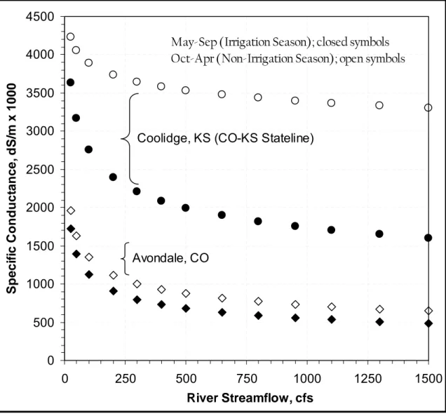
Figure 1. Spatial variation of surface water salinity in the Arkansas River Drainage Basin. Looking closer in Figure 4 the relationship between river streamflow and specific conductance comparing the irrigation season and non-irrigation season is significantly different for an upstream location (Avondale) as compared to a downstream location (Coolidge). During the non-irrigation season and low native surface flow the higher proportion of groundwater return flow to the river accounts for the overall streamflow and high specific conductance at the downstream location.
0.0 10.0 20.0 30.0 40.0 50.0 60.0 0.0 10.0 20.0 30.0 40.0 50.0 60.0
Total Electrolyte Concentration (Cations), meq/l (m molesc/l)
T o ta l A n io n s , me q /l (m mo le s c /l ) 1965-1984 1990-1993 Figure 2 y = 733.09x1.1357 R2 = 0.9986 0 500 1000 1500 2000 2500 3000 3500 4000 4500 0.0 1.0 2.0 3.0 4.0 5.0 Specific Conductance, dS/m T o tal D isso lved S o li d s ( T D S ), m g /l 1965-1984 1990-1993 Figure 3
0 500 1000 1500 2000 2500 3000 3500 4000 4500 0 250 500 750 1000 1250 1500 River Streamflow, cfs Spe c if ic C onduc ta nc e , dS/ m x 1 0 0 0 Avondale, CO
Coolidge, KS (CO-KS Stateline)
May-Sep (Irrigation Season); closed symbols Oct-Apr (Non-Irrigation Season); open symbols
Figure 4. Relationship between river streamflow and specific conductance during periods of the year for an upstream location (Avondale) as compared to a downstream location (Coolidge).
MANAGING FOR SUSTAINED CROP PRODUCTIVITY AND WATER RESOURCE
PROTECTION
As an anthropogenic cause of salinity, irrigation has a profound effect on introducing soluble salts into irrigated agroecosystems. There are four rules regarding irrigation and salinity that need to be understood:
• RULE #1: ALL waters used for irrigation contain salts of some kind in some varying amount.
• RULE #2: Salinization of soil and water is inevitable to some extent.
• RULE #3: An irrigated agroecosystem cannot be sustained without drainage, either natural or artificial. • RULE #4: Rules 1 through 3 can’t be changed.
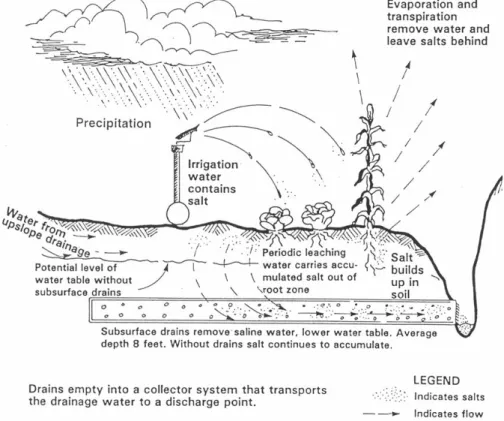
Figure 2 illustrates the salinization process in irrigated terrestrial system and is described as follows. The anthropogenic salinization process by irrigation is driven by evapotranspiration. The concentrations of soluble salts increase in soils as the soil water is removed to meet its
atmospheric demand by evaporation and transpiration. The salts, which are left behind as a consequence of plant uptake of nearly pure water concentrate in the shrinking soil-water volume are added to the existing quantity of salt in the root zone with each successive irrigation that is applied and passed through the soil profile. As an example, an irrigation source with a salt content of 850 ppm is introducing 1.16 tons of salt for every acre-foot of water applied.
Figure 5. Mechanics of the salinization process in irrigated cropland systems (adapted from Tanji, et al., 1986).
Furthermore, soils with shallow, saline water tables can become salinized as the result of the upward flux, probably more familiarly known as capillary rise, of water and salt into the rootzone. Simply stated, these shallow water tables result when the natural discharge is less than the
irrigation-induced recharge. There is a very close correlation between the level of salt accumulation in the soil with the water table depth, the salt content of the groundwater, and the soil’s hydraulic properties. It is these soluble salts, that, if not leached, managed, and disposed of properly with drainage, will eventually build up in irrigated soils to the point that crop yield is adversely affected. There is not usually a single prescription for an effective salinity management strategy. Rather, different practices and approaches need to be combined into a management scheme that is satisfactory in addressing an existing salinity problem or preventing one from manifesting itself into the terrestrial system. A given solution to a salinity problem can be complex. Not only are there the hydrogeology and edaphic, factors but economic and social factors to be carefully considered. The following discussion outlines an important guiding principle and its elements in the
development and adoption of appropriate management strategies.
Since it’s the chemical composition of the irrigation water that creates the adverse soil condition to begin with it seems logical to form a problem-solving framework starting with assessing the given water’s suitability for use. In this regard perhaps the one overarching guiding principle that the practitioner needs to understand in order to develop the most effective salinity control strategy for a given situation should be evaluated on the basis of the potential use of a given source of water. Simply stated the principle is as follows:
“Water has no intrinsic quality, except in the resource setting for which it is to be used. The suitability of any given water source relies strictly on what can be done with it under the specific conditions of use.”
In as much there are several important elements in the development and adoption of appropriate management strategies within this cornerstone principle. These essential elements are (1) grow suitable salt tolerant crops, (2) use planting and tillage procedures that prevent excessive salinity accumulation in the seedbeds, (3) deliver irrigation water to fields efficiently, (4) apply irrigation water in an efficient manner that minimizes the leaching fraction and resulting deep percolation, (5) provide adequate drainage, and (6) monitor irrigation adequacy and soil profile salinity.
Grow Suitable Salt Tolerant Crops
The adverse effects of salts on plants are generally divided into three parts; 1) the osmotic effect (total salt effect), 2) specific ion effects, and 3) the indirect effects caused from soil dispersion due to excess sodium. The emphasis of this section is directed at the first two categories; osmotic effects and to lesser importance the tolerance of plants to foliar salt injury caused by specific ion effects. The indirect soil dispersion effect and the management of infiltration problems will be addressed in a later section.
Osmotic Effect. The plant extracts water from the soil by exerting an absorptive force in response to a gradient along the soil-plant-atmospheric-continuum; one that is greater than that adsorptive force that holds water within the soil matrix. When the plant cannot exert enough energy to extract sufficient water from the soil matrix the plant develops water stress.
Similarly, as the salt concentration of the water within the soil matrix increases, the energy that the plant needs to exert also increases. Increased salt concentrations narrows the gap between the soil water and internal plant energy potential. This is referred to as the osmotic effect caused by the increase in the osmotic potential of the root-zone soil solution. In order to maintain a suitable energy gradient for water uptake to occur, non-halophytes (glycophytes) require additional expenditure of metabolic energy. This additional energy expenditure shift would normally go to building dry matter and other plant functions.
For our purposes here, soil salinity is expressed as the mean electrical conductivity of a saturated-soil extract of the root zone, ECe(avg). The SI unit expressing electrical conductivity is decisiemens per meter. The osmotic potential (bars) of the root zone soil water at field capacity can be
approximated with the relation, OPfc= -0.725ECe(avg)1.06.
All crop plants do not respond to salinity in the same way; some produce acceptable yields at higher soil salinity levels than others do. Each crop species has an inherent ability to make the needed osmotic adjustments enabling them to extract more water from a saline soil. This ability for some crops to adjust to salinity is extremely useful. In areas where the accumulation of salinity within the soil profile cannot be controlled at acceptable levels, an alternative crop can be selected that is more tolerant resulting in the production of better economical yields.
Yield Response Functions. The relative salt tolerance of most agricultural crops is known well enough to provide general guidelines about salt tolerance for making management decisions. The salt tolerance of any given crop can best be illustrated by plotting the potential yield, sometimes referred to as the relative yield, as a function of soil salinity. The potential yield (Yr) or relative yield, expressed as a percent, is defined as the yield under saline conditions (Ya) relative to the yield under non-saline conditions (Ym):
Yr= (Ya/Ym)100 (1)
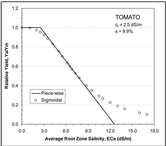
Although it has been shown that the relation between potential yield and soil salinity follows a sigmoidal curve, a piece-wise linear response function is used to easily describe the potential yield/soil salinity relation for acceptable crop yields (Figure 3). Two intersecting straight-line segments represent this linear piece-wise response function. One of the segments has a slope of zero. This means that the yield potential is constant across a range of soil salinity. The second line segment is a salinity-dependent line whose slope describes the yield reduction per unit increase in soil salinity. The point where the two line segments intersect specifies the threshold soil salinity (ECe(ct)) or the maximum average root zone soil salinity at which yield reductions will not occur. Yield reductions will occur when soil salinity levels exceed this threshold value. Mathematically, this piece-wise function can be represented as follows:
When, ECe(avg) is greater than or equal to ECe(ct),
Yr= 100- b(ECe(avg)-ECe(ct)) (2)
and when,
ECe(avg) is less than ECe(ct),
where b is the slope of the second line segment expressed as the percent yield decrease per unit increase in soil salinity, ECe(avg).
0.0 0.2 0.4 0.6 0.8 1.0 1.2 0.0 3.0 6.0 9.0 12.0 15.0 18.0
Average Root Zone Salinity, ECe (dS/m)
R e la ti v e Y ie ld , Y a /Y m Piece-wise Sigmoidal
TOMATO
ct = 2.5 dS/m s = 9.9%Figure 6. Yield response to soil salinity for tomato.
Rearranging Equation 2 the soil salinity at which a given yield potential can be obtained may also be calculated:
ECe(avg)= (100+bECe(ct)-Yr)/b (4)
Likewise, the slope (b) of the line can also be calculated by rearranging Equation 2,
b= 100/(ECe(avg)[0% Yield]-ECe(avg)[100% Yield]) (5) where ECe(avg)[0% Yield] and ECe(avg)[100% Yield] are soil salinities at 0 yield potential and 100% yield potential, respectively. The analysis of tolerance field data shows that crops with similar tolerances form groups. The upper boundaries and relative tolerance rating have been assigned to these groups as shown by the thick-segmented lines (Figure 4). The four (4) regions between the lines define specific divisions for relative crop salt tolerance. These groups are classified as
sensitive (S), moderately sensitive (MS), moderately tolerant (MT), and tolerant (T). Field soil salinity values that fall beyond the dotted line are considered to be unsuitable for most crops of economic importance. 0.0 0.2 0.4 0.6 0.8 1.0 0 5 10 15 20 25 30 35
Average Root Zone Salinity, ECe (dS/m)
R e la ti v e Y ie ld , Y a /Y m Sensitive Moderately Sensitive Moderately Tolerant Tolerant
S
MS
MT
T
Figure 7. Crop yield response to salinity and categories for classifying salinity tolerance. Although these groups are arbitrary, they are particularly useful in those instances where insufficient field data for a crop is available, but a relative rating can be assigned based on field experiences and local observations. The yield response of a crop that has been given a relative tolerance can be then be described (Table 1).
Table 1. Relative crop salt tolerances.
Relative Crop Salinity Slope (b)
Tolerance Rating ECe(avg) [0% Yield] ECe(avg) [100% Yield] [Equation 5] --- dS/m --- -% per dS/m -
Sensitive (S) 7.0 1.3 17.5
Moderately Sensitive (MS) 16.0 3.0 7.7
Moderately Tolerant (MT) 24.0 6.0 5.6
Appendix 1 lists the salinity thresholds (ECe(ct)) and slopes, (b) for the most common crops and plants. In addition, these species have been rated as sensitive (S), moderately sensitive (MS), moderately tolerant (MT), and tolerant (T). The reader is referred to Maas (1990) for an expanded list of crops and their salinity tolerance.
It has been suggested that using the piece-wise linear relation is somewhat flawed (Shannon and Grieve, 1999). The reasons cited are that (1) there’s a significant error in evaluating the slope near the threshold, that few studies include treatments to accurately determine the threshold value, and (2) the slope decreases with increasing soil salinity at the upper end of the curve. One of the more popular sigmoidal models for quantifying crop salt tolerance has been the logistic model that incorporates the parameter representing the salinity (dS/m) at which the yield is reduced by 50%, designated as C50 as presented by van Genuchten and Hoffman (1984). The general logistic model numerical expression takes the form, then, as:
Yr = 1/(1+ (C/C50)p) x 100 (6)
where C is the soil salinity expressed as ECe. When too few data points are available to precisely evaluate the salinity threshold, the value of C50 and p, a crop dependent constant determining the curves shape, provides a more definitive and stable characterization of the yield response to salinity. However, the values of C50 and p have been evaluated for a limited number of crops. It is important to note that for the most part the threshold soil salinity values that are cited were established from field studies where chloride was the predominant anion. In preparation of saturated-soil extracts in the laboratory, gypsum (CaSO4) will be dissolved. For soils that are dominated by gypsum, the ECe(avg) may range from 1 to 3 dS/m higher than non-gypsiferous soils at the same moisture content and electrical conductivity of the soil water, ECsw. This means that values of ECe(ct) for crops grown on soils dominated by gypsum may exceed table values by as much as 2 dS/m.
If the soil salinity levels greatly exceed the tolerance of all of the crop selections options and yield potentials of less than 100 percent are not acceptable, "reclamation" leaching may be necessary prior to any cropping. There are two conditions where reclamation leaching are most likely to be neccesary. The first condition is where an inverted soil salinity profile (accumulated salts decreases with soil depth) has developed. This condition is most familiar where salts have
accumulated in the presence of a shallow water table. The second condition is where a regular soil salinity profile (accumulated salts increases with soil depth) exists at excessive levels caused by inadequate leaching. The goal of reclamation leaching must be to reduce the salt concentration in the upper portion of the root zone to a level that approaches the crop tolerance.
Susceptibility of Crops to Foliar Salt Injury Due to Sprinkler Irrigation. Foliar salt injury has been observed on a number of crop species. Similarly to the varying response of crops to soil salinity, species vary widely in their response to this injury from sprinkler irrigation utilizing saline waters. The foliar injury, commonly referred to as "salt burn", is caused by leaf absorption of excess concentrations of sodium and chloride.
Of all crop species evaluated, citrus and deciduous fruit trees, like apricot, plum, and almond, are the most susceptible to foliar injury. The extent of the injury may go beyond considerable leaf
necrosis and may also include leaf defoliation. Among the herbaceous crops, plants’ belonging to the Solonaceae family is generally the most sensitive. This would include potato, tomato, and peppers.
Table 2 provides some general guidelines for determining the susceptibility of crops to foliar salt injury from sprinkler irrigation based on the concentrations of sodium or chloride. These data represent field studies where the sprinkling occurred during daytime hours. There appears not to be a correlation between a crops tolerance to soil salinity and its susceptibility to foliar injury. Two examples include strawberry and avocado; both are very salt sensitive crops, but field data shows the risk of foliar injury to be negligible. Changes in management have been shown to reduce the risk of foliar salt injury. These include irrigating at night, avoiding periods of hot, dry winds, increasing sprinkler droplet size, and increasing rates of application.
Table 2. Tolerance of crops to foliar salt injury from water applied using sprinkler irrigation methods.
Critical Sodium (Na+) or Chloride (Cl-) Concentrations (meq/l)
Tolerant Sensitive
>20 10-20 5-10 <5
Cauliflower Alfalfa Grape Plum
Sugarbeet Sorghum Pepper Citrus sp
Cotton Safflower Tomato Almond
Sunflower Barley Potato Apricot
Corn
Stages of Growth. The soil salinity/crop tolerance relations in Appendix 1 apply primarily to responses from the late seedling growth stages to maturity. Field data on the variable crop tolerance during the early stages of growth (i.e. germination, emergence and seedling growth) are extremely limited. As a general rule most plants are tolerant during germination. After
germination, plants may then become sensitive during emergence and the development of the seedling. Past studies have shown that increased salt concentrations may delay emergence, but does not affect final emergence. However, secondary conditions such as soil crusting could result in reduced crop stands. A general recommendation is that a soil salinity level of 4 dS/m in the seed zone will delay emergence seedling growth.
Use Planting and Tillage Procedures that Prevent Excessive Salinity
Accumulation in the Seedbed
A number of crops tend to be sensitive to salinity during germination and seedling establishment. Stand losses can occur particularly when raised beds or ridges are employed. These losses can be significant even when the average salinity levels in the soil and in the irrigation water are moderately low particularly under furrow irrigation. Since salts move with the water, the salt accumulates progressively towards the surface and center of the raised bed or ridge. Thus the
greatest damage occurs when a single row of seeds is planted in the middle of the bed. This is so because salts tend to accumulate under furrow irrigation in those regions of the seedbed where the water flows converge and evaporate this problem is magnified when saline waters are used for irrigation (Bernstein and Fireman, 1957).
Seedbed planting systems and furrows need be designed to minimize this problem. This can be accomplished by considering alternative bed-furrow configurations and irrigation practices that involve seedbed shape, seed placement and irrigation techniques including alternate furrow irrigation. Figure 3 illustrates typical salt patterns in flat and sloping beds.
Figure 8. Salt accumulation patterns of flat and sloping beds as influenced by irrigation practice (Adapted from Bernstein and Fireman, 1957; Bernstein, et al., 1955).
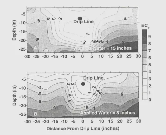
With the expansion of the use of subsurface drip irrigation in the Arkansas River basin, it is important to consider the distribution of salts within the root zone and bed. The patterns that form under subsurface irrigation are distinct and differ significantly from the pattern where the drip tubing is on the soil surface. Common to both cases salinity gradually increases as the horizontal
distance from the line increases and the greatest salinity occurs at the leading edge of the wetting front very high salinity levels can occur near the soil surface (Figure 9).
While adequate leaching occurs below the buried tubing, the accumulation of salts above the drip tubing presents a dilemma. A salinity hazard can develop if insufficient non-crop season
precipitation occurs and moves the surface soil accumulated salts back into the immediate seed zone that can be detrimental to the subsequent year’s crop. One strategy is to leach the salts with sprinkler irrigation.
Figure 9. Root zone salt distribution with subsurface drip irrigation system.
Deliver Irrigation Water to Fields Efficiently
Unmistakably, the strategy for sustaining crop productivity and reducing the risk of salinity hazards of irrigated lands requires good irrigation management. The basis for good irrigation management for salinity control is timely uniform irrigations, applied in an adequate quantity to meet the crop’s consumptive use (evapotranspiration) and at the same time satisfy the leaching requirement. In addition, the causal and interacting elements of good irrigation water management include the delivery system and the method and manner of irrigation. For example water delivery based on predetermined amounts or preset periods without consideration of seasonal variations generally encourages over-irrigation. A consequence of these institutional constraints is limited adoption of higher efficient irrigation such as sprinkler and drip. The optimum water delivery infrastructure is one that can provide metered, controlled water nearly on a continuous basis so that the soil water content in the rootzone can be kept within prescribed limits.
The other two factors that must be considered as an overall strategy are controlling (i) seepage losses and (ii) maintaining drainage systems. Excessive loss of irrigation water from canals constructed in permeable soil contributes to not only the mineral dissolution of the underlying geologic materials, but contributes significantly to the manifesting of high water tables and soil salinization. Every effort should be taken to minimize these seepage losses.
The maintenance of the drainage system is also a key factor. Both in-field tile lines and open drains should be kept in working order. As far as sustaining irrigated agriculture it may well be necessary to reactivate many of the drainage districts in the basin.
Apply Irrigation Water in an Efficient Manner that Minimizes the Leaching
Fraction and Resulting Deep Percolation
As discussed earlier some salt accumulation is inevitable attributed to two processes. Salt loading occurs from mineral weathering and dissolution of soluble salts. Moreover, salt concentration occurs from plant uptake of water driven by evapotranspiration, thus leaving the salts behind. When the accumulation of salts in the soil root zone becomes excessive to the point of affecting crop yield, they can easily be leached in the absence of a water table. The goal is to move a portion of the salts below the root zone (deep percolation) by passing irrigation water through the root zone.
The ability to pass a specific volume of water through and passed the root zone is dependent on sufficient water-entry at the soil surface or infiltration. The negative effect of salinity, specifically the amount of calcium and magnesium, relative to the amount of sodium is the interference in the normal infiltration rate and subsequent percolation of the infiltrated water (also referred to as permeability) through the vadose zone. When an infiltration problem results from the deleterious effect of the adsorbed sodium it is most commonly referred to as a sodium hazard or “sodicity”. This section discusses the leaching fraction (LF), the proper calculation of the LF and assessing sodium hazards.
Leaching and Deep Percolation. Clearly, if the volume of water applied can be minimized in a quantity not to exceed a crop’s requirement, then the amount of salt added to the soil can be minimized. For example, water immediately below John Martin Reservoir contains about 3.3 tons of salt for every acre-foot of water diverted.
Leaching, as the key factor in controlling the soluble salts, is accomplished by applying an amount of water that is in excess of the crops seasonal evapotranspiration and runoff. This excess amount of water is called the leaching fraction (LF), normally expressed in the decimal form. As an
example, a LF of 0.5 means that 50% of the water infiltrating into the soil profile passes through and out of the root zone.
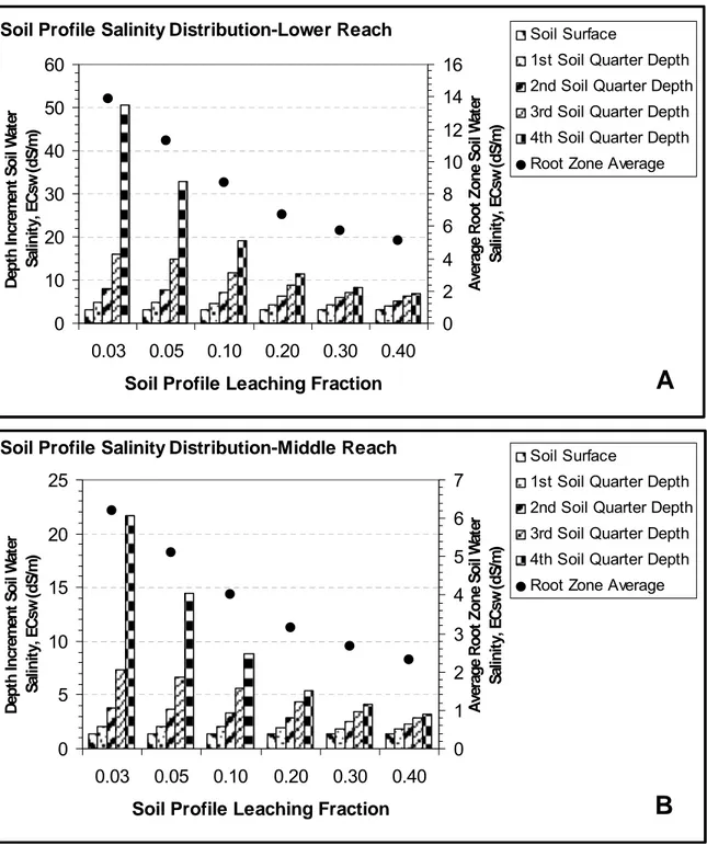
The strategy is to optimize the leaching fraction to an acceptable minimum. The basis for attaining a minimum LF is two-fold. First as the LF decreases the precipitation of the dissolved salts applied in the irrigation water increases. The precipitation of salts consists of calcium, bicarbonate, and sulfates as carbonates and gypsum. The salt precipitation results in a decrease of the amount of salt in the soil and subsequent discharge from the rootzone. Second, reducing the amount of water passing through the root zone reduces the risk of additional dissolution of weathered minerals from substrata from the percolating water. The extent to which the LF can be minimized is limited by (i) the irrigation system, (ii) a crop’s tolerance to an increase in the root zone salinity. To demonstrate the effect of leaching fraction on soil profile salinity, an example is given using the expected dissolved salt constituents of water diverted at two different landscape positions and six
different leaching fractions. Figures 10a and 10b compare the soil profile salinity distribution and the precipitation-dissolution of gypsum when irrigated with water composition expected of that below John Martin Reservoir compared to that expected between John Martin and Pueblo Reservoirs.
Soil Profile Salinity Distribution-Lower Reach
0 10 20 30 40 50 60 0.03 0.05 0.10 0.20 0.30 0.40
Soil Profile Leaching Fraction
D ep th In cr em en t S oil W at er Sa lin ity , E C sw (d S/ m ) 0 2 4 6 8 10 12 14 16 A ver ag e R oo t Z on e S oil W at er Sa lin ity , E C sw (d S/ m ) Soil Surface
1st Soil Quarter Depth 2nd Soil Quarter Depth 3rd Soil Quarter Depth 4th Soil Quarter Depth Root Zone Average
A
Soil Profile Salinity Distribution-Middle Reach
0 5 10 15 20 25 0.03 0.05 0.10 0.20 0.30 0.40
Soil Profile Leaching Fraction
D ep th In cr em en t S oi l W at er Sa lin ity , E C sw (d S/ m ) 0 1 2 3 4 5 6 7 A ver ag e R oo t Z on e S oil W at er Sa lin ity , E C sw (d S/ m ) Soil Surface
1st Soil Quarter Depth 2nd Soil Quarter Depth 3rd Soil Quarter Depth 4th Soil Quarter Depth Root Zone Average
B
Figure 10. Soil profile salinity distribution as a function of the leaching fraction for the (A) lower reach and (B) middle reach of the Arkansas River basin.
Below John Martin Reservoir (Figure 4a) the leaching fraction increases as the average expected soil ECe in the absence of a water table decreases ranging from 6.9 dS/m at a 3 percent LF to an ECe of 2.5 dS/m at LF equal to 40 percent. [Note that the ECe is about half of the EC of the soil water.] Above John Martin (Figure 4b) the average expected soil ECe in the absence of a water table ranges from 3.1 dS/m at a 3 percent LF to an ECe of 1.2 dS/m at LF equal to 40 percent. This illustrates the greater potential of reducing the leaching fraction of waters within the middle reach. To keep the salts balanced so that the soil profile ECe is equal to 2.5 (ECw= 5) we can minimize the LF to 40 percent and 5 percent using water diverted below and above John Martin Reservoir, respectively.
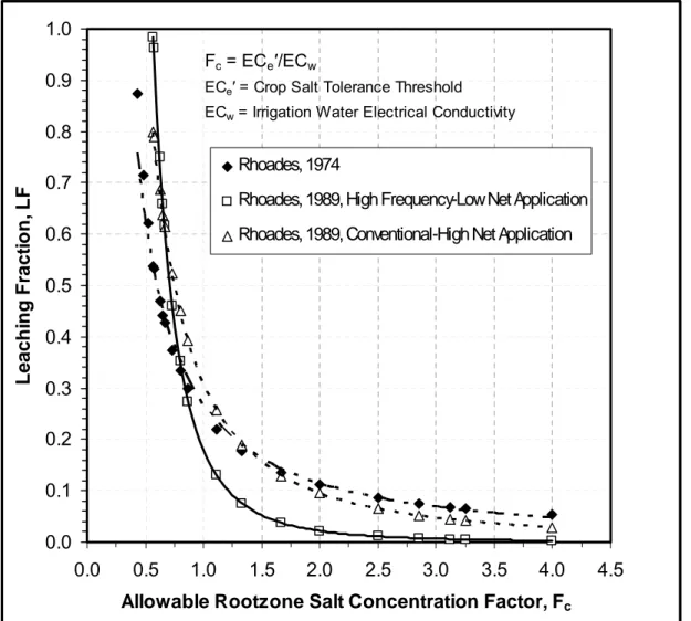
Leaching Fraction Estimation. In order to estimate the LF and the amount of water required, only three pieces of information are needed; (i) the crop threshold soil salinity, ECe(ct), (ii) the salinity of the irrigation water, ECw, and (iii) seasonal maximum evapotranspiration (ETm) of the crop. Figure 7 shows the relation between the leaching fraction, LF, and the ratio, Fc.
0.0 0.1 0.2 0.3 0.4 0.5 0.6 0.7 0.8 0.9 1.0 0.0 0.5 1.0 1.5 2.0 2.5 3.0 3.5 4.0 4.5 Allowable Rootzone Salt Concentration Factor, Fc
L e a c hi ng Fr a c ti on , L F Rhoades, 1974
Rhoades, 1989, High Frequency-Low Net Application Rhoades, 1989, Conventional-High Net Application
Fc = ECe′/ECw
ECe′ = Crop Salt Tolerance Threshold
ECw = Irrigation Water Electrical Conductivity
Figure 11. Relationship between the allowable rootzone salt concentration factor, Fc, and the leaching fraction, LF.
This ratio (Fc) is the crop threshold salinity divided by the irrigation water salinity (Fc= ECe(ct)/ECw). This relation shows that for any particular crop, the LF exponentially increases as the salinity of the water increases (ratio decreases).
Knowing the threshold salinity, ECe(ct), for a given crop and the electrical conductivity of the irrigation water, ECw, the necessary leaching fraction (LF) can be graphically determined from Figure 11. For a more accurate LF estimation the exponential relations shown in Figure 11 can be simplified for any particular crop. The “classical” method (Rhoades, 1974; Ayers and Westcot, 1985) of determining the LF is described by the following equation:
LF= ECw/(5ECse(ct) - ECw) (7)
where ECse(ct) is the average ECe at which the yield potential is 90% or greater.
In recent years (Rhoades, et al., 1989) it has been shown that the LF is affected by the net water application. To account for this effect an alternative method of determining the LF has been developed based on the allowable root zone concentration factor, Fc. Since the net water application can be related to the irrigation system these relations are divided into two categories, namely (i) conventional and (ii) high frequency. Under "conventional irrigation" where there are relatively large net water applications, a higher leaching fraction is required at the same value of Fc as compared to high frequency irrigation (small net water applications). Conventional irrigation scenarios where net water applications are relatively large include deep rooted crops grown under surface irrigation. High frequency irrigation scenarios include shallow rooted crops under surface irrigation or where sprinkler or drip irrigation systems are used.
The exponential relations for the conventional irrigation (Cl) and high frequency irrigation (HF) can be calculated as follows:
LF= 0.1794/(Fc)3.0417 (High Frequency Irrigation-HF) (8) LF= 0.3086/(Fc)1.7020 (Conventional Irrigation-Cl) (9) The net annual depth of irrigation water (Dw) that is required to meet both the crop
evapotranspiration (ETm) and the leaching requirement, Dsw′ (excluding runoff) is equal to:
Dw = ETm + Dsw′ (10)
Relative to the crop’s total annual evapotranspiration the net annual depth of irrigation water can then be calculated:
Dw = ET/(1-LF) (11)
where the ET and Dw are expressed in inches. From Equation 10, the portion of water that is applied for the leaching can then be calculated as:
Dsw′ = Dw - ET (12)
or,
Field studies and observations have shown that as a general rule the timing of leaching is not critical as long as the crop tolerance threshold is not exceeded during critical periods or extended time periods. Alternative timings include every irrigation, at selected seasonal irrigations or less frequently. It must be noted that water losses attributed to deep percolation that occur during the season, particularly with surface irrigation systems, are often in excess of the leaching fraction. A careful analysis must be done to determine whether or not the amount of water required for salt leaching will be satisfied by the field's irrigation inefficiency.
Infiltration and the Sodium Hazard. Salinity and sodicity affect soil structure in which the aggregate stability provides a network of conducting pores or optimum infiltration and permeability to take place. As previously introduced, a negative effect of salinity and the amount of sodium is the interference in the normal infiltration rate and subsequent percolation of the infiltrated water (also referred to as permeability) through the vadose zone. In the presence of sodium surface crusting, swelling, and dispersion are the primary processes responsible for an infiltration problem occurring In the presence of sodium which is reflected in the reduction in the soils hydraulic conductivity.
The soil’s sodicity can be described based on the exchangeable sodium ratio (ESR) or the more familiar term; the exchangeable sodium percentage (ESP) which is the percentage of the total exchange complex (or cation exchange capacity, CEC) saturated with sodium. Although the sodium hazard is a direct function of the soils exchangeable sodium percentage (ESP) the sodium adsorption ratio (SAR) of the soil solution is the variable that is used to describe the sodic condition since the SAR is more easily ascertained.
0 5 10 15 20 25 30 0.0 1.0 2.0 3.0 4.0 5.0 6.0
Electrical Conductivity of Infiltrating Water, dS/m
Sodi um A d s o rp ti on R a ti o a t S o il Sur fa c e Area of unlikely
permeability hazard (No reduction in infiltration rate)
Area of likely permeability hazard (Reduction in infiltration rate)
Figure 12. Soil permeability hazard as influenced by salinity of infiltrating water and sodium and SAR.
In review, we said that the two factors that affect water infiltration are the (1) water’s salinity and, (2) its sodium content in relation to the content of calcium and magnesium. The following general precepts are good few rules of thumb to remember:
• High salinity water (i.e. high EC) increases infiltration
• Conversely, low salinity water (i.e. low EC ) decreases infiltration
• Water with a high sodium content relative to the calcium and magnesium content (i.e. high SAR) decreases infiltration.
The principle to keep in mind is that both factors, the salinity of the water and sodium content, operate at the same time. In other words, just because a certain water’s electrical conductivity (ECw) is low or the water’s SAR is high doesn’t necessarily mean that an infiltration problem will be manifested. This can be thought of in another way. That is to say that if there is sufficient calcium to offset the dispersing effect of the excessive sodium and that the total electrolyte concentration of the applied water is above the critical flocculation concentration, the soil pore sealing and soil dispersion causing reduced infiltration is unlikely.