The Puzzle between Economic Growth and Income Inequality

(1)

The Puzzle between Economic

Growth and Income Inequality

December 2013

Bachelor’s Thesis in Economics

Authors: Mahmood Jamal

Omar Sayal

Tutors: Scott Hacker

Mark Bagley

(2)

Acknowledgment

We would like to express our great appreciation to our supervisors, Scott Hacker and Mark Bagley, for their valuable support, encouragement and advices for writing this thesis.

(3)

Bachelor’s Thesis in Economics

Title: The Puzzle between Economic Growth and Inequality Authors: Mahmood Jamal

Omar Sayal

Tutors: Scott Hacker (Supervisor) Mark Bagley (Deputy Supervisor) Date: December 2013

Keywords: Income inequality, economic growth, Gini index, Lorenz curve, Kuznets curve, cross-sectional

Abstract

The purpose of this paper is to investigate the correlation between income inequality and economic growth in a cross-section of 90 countries from 2002 to 2006. The controversial Kuznets Hypothesis, the economic model that hypothesizes the relationship between inequality and per capita income is an inverted U-shaped curve, is scrutinized and investigated to consider its viability and accuracy. A multiple linear regression model is estimated and the viability of the regression model is supported by several statistical tests. Based on the estimated model, a negative correlation between growth and inequality has been found.

(4)

1. Introduction ... 1

1.1 Purpose ... 2

1.2 Disposition ... 2

2. Measuring Inequality ... 3

2.1 Lorenz Curve and the The Gini index

...

3

3. Theoretical Framework ... 5

3.1 Kuznets Hypothesis ... 5

3.2 Other Economic Theories on the Linkage between Growth and Inequality ... 6

4. Previous Studies on Growth and Inequality ... 7

4.1 The Puzzle between Growth and Inequality ... 7

4.2 The Existence of the Inverted U-curve ... 7

4.3 Criticism of the Inverted U-curve ... 8

4.4 Criticism of the Mechanistic and Casual Relationship between Growth and Inequality ... 9

5. Empirical Framework and Findings ... 11

5.1 Investigating the Kuznets curve... ... ……...11

5.2 Method and Model ... 12

5.3 Descriptive Statistics ... 14

5.4 Data... ... ....15

5.5 Regression Results ... 16

5.6 Tests of the Regression ... 17

5.7 Discussion……… ... .19

6. Conclusion ... 20

6.1 Suggestion for Further Research ... 21

(5)

Figures

Figure 1: Graphical presentation of The Gini index coefficient………...…..…...4

Figure 2:Plotting the Lorenz curve………..4

Figure 3: Hypothetical Kuznets curve……….5

Figure 4: Scatter plots of income per capita vs.The Gini index………...……...11

Figure 5: Income category and the Kuznets curve……….………12

Figure 6: Residual plots of The Gini index and growth……….……….18

Tables

Table 1: Countries’ classification………...………13

Table 2: Variables' definition………..…14

Table 3: Descriptive statistics……….15

Table 4: Regression results of dependent vs. independent variables………...16

Table 5: Variance Inflation Factors...17

Table 6: Heteroscedasticity’s White test……….….18

Appendix

Appendix 1: Income data distribtution...24

Appendix 2: The value of The Gini index for each country…. ………..28

Appendix 3: The list of the classified countries with corresponding PPP………29

Appendix 4: The descriptive statistics...30

Appendix 5: Regression results……….31

Appendix 6: Regression results with two additional variables………..……31

Appendix 7: The correlation matrix...32

(6)

1. Introduction

All animals are equal, but some animals are more equal than others. George Orwell, Animal Farm

During the course of history, many thinkers, philosophers and economists have been occupied with the issue of inequality and inequality in income distribution. Inequality in many societies have caused great wars and revolutions such as the French Revolution (1789-1799), the Russian Revolution (1917) and the Chinese Revolution (1949) that had great, fundamental and far-reaching impacts on many countries and schools of thoughts. Egalite (equality) was one of the three mottos of the French Revolution. The famous French writer, Honore De Balzac, was so frustrated with the situation to write that “behind every great fortune is a crime.”

Even before the French thinkers, such as Saint-Simon and Fourier who raised the issue of inequality, Plato, the Greek philosopher, said that “any city, however small, is in fact divided into two, one the city of the poor, the other of the rich; these are at war with one another.” Economic inequality has an important and sacred place on people’s beliefs and trust about fairness and justice in society. Ethically people do not favor sharp inequalities in income, wealth and other resources of society such as public services and opportunities because of its dire consequences and impacts on society in general. High inequality can deteriorate and harm outcomes such as health, school attainment, longevity, personal achievements, etc. Wilkinson (1996) points out that people who live in countries with high income inequality may experience worse health than those who live in countries with low income inequality. When income inequality and inequalities in other fields produce undesirable outcomes for individuals in particular and for the society in general, one must investigate why they arise. The recent turmoil in the Middle East and North Africa, also known as the Arab Spring that started on December 2010, is deeply related, among other factors, to inequality and poverty in those societies. And when on September 2011 the Occupy Wall Street movement began, its slogan, “the 99 percent”, was the stark demonstration of the Americans anger against the sharp inequalities in the US.

However, despite the economic development and GDP growth in many countries around the world since the industrial revolution, particularly in the developed countries, and despite the reduction in poverty rate in some countries recently, the income inequality, against conventional wisdom (Kuznets Hypothesis), has increased even in those countries that had have to experience reduction in inequality because of the enormous economic growth. Saez’s joint work with Piketty, which tracks the incomes of the poor, middle class and the rich around the world, shows that top earners in the US have taken an increasingly larger share of the overall income during the past three decades. Their findings show that average real income per family in the US from 2009 to 2012 grew modestly by 6.0%. “Top 1% incomes grew by 31.4% while bottom 99% incomes grew only by 0.4% from 2009 to 2012. Hence, the top 1% captured 95% of the income gains in the first three years of the recovery” (Saez, 2013). The gap between the top 10% earners and the bottom 90% earners also widened in some other countries of the world (see Appendix 1 for more details).

(7)

economic growth and income inequality pioneered the way for a number of other researchers and economists to study the relationship between the two. The results of the studies can be categorized into three wide-ranging groups: (1) positive correlation between growth and inequality, (2) negative correlation between growth and inequality and, (3) no systematic correlation between the two. This paper studies the relationship between growth and income inequality that has been measured by the Gini index in a panel of countries from 2002 to 2006. We have categorized the countries under study into three different categories, i.e. high income, middle income and low income.

In our investigation, particularly on the analysis part, we have born in mind that growth is not the only explanatory variable for the increasing or decreasing trends in inequality in different countries that are in their different phases of economic and socio-political development. There are many other factors that can fundamentally influence both growth and inequality which have been briefly discussed in the theoretical and previous studies sections of this paper.

1.1 Purpose

The purpose of this paper is to study the relationship between growth and income inequality. The Kuznets Hypothesis will be investigated using data across many countries to find if there is any correlation between growth and income inequality. The paper also will attempt to find the nature of that correlation, i.e. whether is it a negative or a positive correlation.

1.2 Disposition

Section two provides information about the measurement of inequality and the Gini index that has been used in this paper for measuring inequality. The Lorenz curve, plotting the Lorenz curve and graphically calculating the Gini index through the Lorenz curve are also covered in this section.

In section three the theoretical framework of the paper is covered. Besides mentioning other relevant theories on the linkage between growth and inequality, the Kuznets Hypothesis (Kuznets curve) is mentioned because one of the main purposes of this thesis is to investigate the Kuznets curve.

Previous studies and findings on the relationship between growth and inequality are mentioned in section four.

In section five, first the relationship between income per capita and the Gini index in a two dimensional approach is graphically investigated. Then the method used for the regression is described. The model is described and the descriptions of the dependent and independent variables are included. The regression, descriptive statistics, and the correlation and the regression analysis are also discussed in this section. Discussion on the results from our investigation on the relationship between growth and inequality is also covered in this section. The analysis is based on the empirical findings of the paper, the theories on growth and inequality and the Kuznets Hypothesis on the issue.

The conclusion in section seven, sums up the purpose and findings of this paper. Suggestions for further research are also mentioned in this section.

(8)

2. Measuring Inequality

In this section of the paper, a brief description of inequality measurement is presented. The main focus is on the Gini index and the Lorenz curve. The main source for this section is Ray (1998).

Income inequality might be visible between two or three different people, but it is more complicated to observe it in situations when two or more regions or countries are compared. Therefore, a measurement is required for comparing and ranking when there are more than two countries or regions. Efforts led to the development of several indices and metrics, such as Hoover index, also known as Robin Hood index, Thiel index, Kuznets ratios and the Range. These measurements are more practical and useful for situations when there is a need to obtain a further insight into inequality. The standard properties for what an index should have are controversial, as there are many indices that have their own properties that produce different results and outcomes. But there are four major criteria or principles that are widely accepted. The Gini index (also known as the Gini coefficient), and the Lorenz curve, which are used in this paper to measure inequality, satisfies all of the four criteria.

These criteria and properties are:

1. Anonymity: When two people earn a different income, both of them are treated equally. No race or profession is treated different from others. Income always could be ranked from the poorest to the richest, i.e. it does not matter who is earning the income.

2. Population: When two populations with different sizes are compared, the size of the population does not affect the outcome. The only difference comes from the proportions of population that earn at different levels of income.

3. Relative Income: Only relative income matters, not absolute income. When comparing two different groups with varying income, the result for each group should be relatively the same. 4. The Pigou-Dalton principle: The Pigou-Dalton principle is an important criterion for measuring inequality. The principle is that transfer of income from the rich to the poor reduces inequality so long as that transfer does not switch the ranking or order between the two. It also maintains that a regressive transfer in income, a transfer from worse-off (poor) to the better off (rich), increases inequality and decreases social welfare.

2.1 The Lorenz Curve and the Gini index

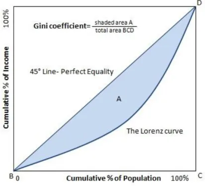
A graphical presentation of an income inequality is useful because it produces a picture that could be easily used for interpretation, comparison and, then, reaching to a meaningful conclusion. The Lorenz curve possesses this characteristic by satisfying the four criteria of the inequality measurement. The Lorenz curve presents the relationship between income and population. As figure 1 shows, the horizontal axis represents the cumulative population and the vertical axis indicates the cumulative income. Both are measured in percentage terms. The graph is split by a 45°line that depicts a perfect equality between the two variables, e.g. when 50% of population corresponds to 50% of income.

(9)

Figure 1: Graphical presentation of the Gini index coefficient

The Lorenz curve initiates at the beginning of the 45° line and ends at the same line. The inequality is depicted by the curve (Lorenz curve), which is bowed downwards. Lorenz curves that are bowed further away from the perfect equality line correspond to those economies that have more inequality. The Gini index is the ratio of the area between the Lorenz curve and the line of perfect equality to the area of the triangle below the line of perfect equality. Mathematically, the Gini index is equal to A/BCD. See figure 1 above for more illustrative details.

In the illustrative example, figure 2, the point (25, 5) represents the (hypothetical) fact that the bottom 25 percent of population have 5% of the income; the point (50, 20) shows that the bottom 50 percent of population have 20% of the income, and the point (75, 40) shows that the bottom 75 percent of population have 40% of the income. However, point (50, 50) shows perfect income equality because 50 percent of population has 50% of the total cumulative income.

There are two problems arising when using only the Lorenz curve for measuring inequality. First, it does not provide a quantitative measure that is more accurate than a graph. And second, it does not allow

rankings as two curves might cross. The Gini index solves these two problems by providing a quantitative measurement that could be used for a deeper accuracy and ranking among several observations. The Gini index is widely applied in the empirical research of inequality due to

(10)

its simplicity. It takes values between 0 and 1. The value of 1 indicates perfect inequality and 0 indicates a perfect equality. Any increase in the value indicates an increase in the inequality level.

Attached to appendix 2 is the value of the Gini index for each country that is used for this thesis.

3. Theoretical Framework

In this section a number of prominent economic theories, which attempt to find the linkage between inequality and economic growth, are covered.

3.1 Kuznets Hypothesis

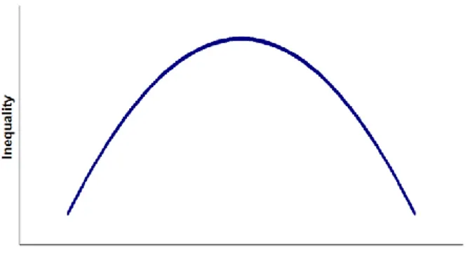
In an influential paper in 1955, the Nobel laureate, Simon Kuznets studied the correlation between economic growth and income inequality and cautiously hypothesized that there is a cycle of inequality caused by market forces. He, after studying and analyzing the historical income distribution data of the United States, England and Germany, found out that during the initial phases of economic growth, income inequality within nations tends to increase, but as the nations’ economies grow and they accumulate more wealth, inequality tends to slow down. Kuznets explains this in terms of shift away from rural/agricultural economy to urban/industrial economy as referred to industrialization and urbanization (Kuznets, 1955). Using both cross-country and time series data, Kuznets (1963) found an inverted U-shaped (known as Kuznets curve) relation between income inequality and GNP per capita, as graphically presented in Figure 3.

Figure 3: Hypothetical Kuznets curve

The Y-axis measures the level of inequality against X-axis which describes the growth of income per capita. So graphically the level of inequality is a function of the level of GDP per capita. As income per capita increases, the level of inequality also increases until a certain turning point (the peak of the inverted U-curve). After this point (threshold), as the income per capita grows due to industrialization and urbanization overtime, inequality follows a downturn slope, i.e. decreases overtime. However, Kuznets (1955) warned that his “paper is perhaps 5 per cent empirical information and 95 per cent speculation, some of it possibly tainted by wishful thinking”.

(11)

3.2 Other Economic Theories on the Linkage between Growth and Inequality

Because of the complexity and interconnectivity of inequality phenomenon with tens of other essential factors, there are many political, social and economic theories that attempt to study and analyze the relationship between growth and inequality. In this paper, we cover only the economic theories that link inequality to growth. Political theories that, for example, emphasize on the development of institutions or political stability for growth (Alesina and Perotti, 1994) or social theories that, for instance, link inequality to growth through education and class prejudice (Perotti 1993 and Basu 2001) are out of the scope of this paper.

Empirical studies have found different trends and results on the impact of inequality on growth or vice versa. Neo-classical economic theories consider incentives essential for growth and therefore they consider some degree of inequality positive for growth. According to Okun (1975), there is a trade-off between equity and growth. While Kaldor (1956) suggests that inequality creates incentives to use the resources in a more productive way, Voitchovsky (2005) connects inequality with innovation, entrepreneurship and risk-taking.

However, Murphy, Schliefer, and Vishny (1989) consider high inequality as not inducive for growth as high inequality reduces aggregate national demand and therefore slows down the process of industrialization and economic growth. Keynes (1936) establishes connection between savings rate and income level. Therefore, if the rich cannot save more, due to redistribution through taxation, the level of investment will be reduced.

Imperfect market characteristics, especially in the credit market, provide theoretical explanation for the linkage between inequality and growth. With asymmetric information and the limitation of legal institutions, such as limited collateral and poor contract enforcement, creditors are reluctant and not eager to issue loans due to the absence of compensation and protection and debtors are not protected in case of bankruptcy. Therefore, these limitations destroy investment potentials and prevent the poor from accessing the capital market, reducing entrepreneurship, investment and growth (Ray, 1993). With the improvement of capital market and legal institutions during the development process, the effects of inequality on economic growth would be larger for the poor countries than the rich ones (Barro, 2000). More access to capital market at the presence of legal institutions and symmetric information would increase the overall level of societal capital, enabling the poor to make investment and increase their wealth. With the accumulation of wealth above a certain level, the wealth will “trickle down” from the rich to the poor because the rich will invest and create jobs for the poor (Aghion and Bolton, 1993).

Banerjee and Newman (1993) argue that if the ratio of very poor to the very rich is high, growth will “run out of steam” and low employment and low wages would be the results. Thus, an economy with a low number of poor people, even in the absence of high per capita income, will grow rapidly and end up in high wage and low unemployment.

Theory within political economy often regards more inequality destructive for growth. Barro (2000) points out that in the model of Alesina and Rodrik (1994), where the relative share of labor and capital endowment is monotonically related to distribution of income as determinants of voting behavior of voters, if the mean income in a country is more than the median income, majority system voting tends towards more redistribution from the rich to the poor. Thus, a greater level of inequality advocates more redistribution through voting (median voter theorem). This consequently will distort economic decisions, such as reducing the amount of investment and high taxation for public projects financing.

(12)

Josten and Truger (2003) propose the fiscal model. In their model, rising inequality leads to redistribution, higher distribution requires more taxation for financing and, finally, more taxation distorts incentives and reduces growth.

4. Previous Studies on Growth and Inequality

In this section a brief review of other research concerning the growth and inequality is presented. Later it will be used in the analysis part to compare previous findings and results with the result of this paper.

4.1 The Puzzle between Growth and Inequality

Over centuries the question of inequality has occupied many researchers in many different fields of social sciences. They have attempted to explain the causes and the consequences of inequality in a society. Paukert (1973) rightly mentions that the notion of inequality has not been just a pure economic concept. Equality before the law, political equality and social equality have been topics appearing in different literatures throughout the history.

In spite of the profound interest on the topic of economic inequality, no systematic work has been carried out to study the concept of income inequality. Even Adam Smith limited his concern to distribution among factors of production and not exactly to the size of income distribution (Paukert, 1973). Influenced by the French Revolution, some Utopian socialists, such as Saint-Simon, Fourier and Owen, raised the question of inequality, but they did not advocate full equality of income. Their views were not coherent as they missed including issues such as merit and need in their treatment of the problem. Also, the whole political economy of Marx is concerned with equality and how to form an equal society.

However, interest in the issue of income distribution regarding size of inequality and the relationship between inequality and economic growth has its origin in the classical article of Simon Kuznets on economic growth and income inequality which led to the relationship’s growing popularity until it came to “acquire…the force of economic law” (Robinson 1976 and Srinivasan 1977). Since then, the interest in the issue has occupied many researchers and economists to study and investigate if the Kuznets U-Hypothesis (Kuznets curve) sustains its validity in different stages of economic development of different countries or not.

4.2 The Existence of the Inverted U-curve

In his research on historical distribution data within the US, UK and Germany, Kuznets (1955) found that with an increase of per capita income, the aggregate inequality within nations will increase at the early stages of growth, but after some turning point (threshold point) and as growth continues and nations become wealthy, income inequality will start to decrease nationwide. Kuznets (1963) found an inverted U-shaped relationship between income inequality and GNP per capita. The result was interpreted as describing the evolution of the distribution of income over the transition from the rural sector with low productivity to the industrial sector with high productivity.

(13)

Theoretically and empirically the Kuznets curve is a controversial issue. “The Kuznets curve is neither a law nor even a central tendency. The pattern is that there is no pattern” (Krueger, 2002). Different researchers have found different results because of the use of more advanced data sets and different functional forms.

In influential papers, Ahluwalia (1974 and 1976) and Ahluwalia, Carter and Chenery (1979) confirm the inverted U-curve. “There is strong support for the proposition that relative inequality increases substantially in the early stages of development, with a reversal of this tendency in the later stages” (Ahluwalia, 1976). They stated that the extent of poverty differs in countries and it depends upon two factors: (1) the average level of income and (2) the degree of inequality in its distribution. Ahluwalia (1976) has argued that in the early stages of growth inequality increases, but it does not offset the effects of growth. Actually, income level of the poorer will rise but slower than the average rate.

However, Ahluwalia, et al. (1979) emphasize that the cross-country relationship should not be regarded as an iron law. Those countries that are able to establish preconditions for more equal distribution of income and create a stimulating environment for growth will be able to either avoid the increase in inequality or moderate the phase of increasing inequality. The fact that the inequality will rise in the initial stage of the growth is, among other things, due to the increasing demand for more skilled labor in the face of a limited supply of skilled labor. This consequently will broaden the gap in wages and result to income inequality (Ahluwalia, et al., 1979).

Barro (2000) conducts panel studies on broad number of countries between 1960 and 1995 and concludes that there is a weak relationship between growth and investment and the level of income inequality. Barro’s studies show the same pattern as Kuznets’s, but in Barro, it is the new technologies that explain the difference between incomes. The old sector tends to use old technologies while the new sector uses the new technologies. The difference will create a gap between the incomes of the two sectors with two different technologies. But as the old sector learns and adopts to use the new technology, the income inequality between the two sectors eventually will decrease.

However, Forbes (2000) challenges the belief that income inequality has a negative relationship with growth. Scrutinizing the previous works by a wide range of researchers, including those by Barro and Deininger and Squire that reject the notion of positive correlation, she argues that measurement error in equality and omitted-variable bias are those analytical problems that resulted to the negation of a positive relationship between growth and inequality by previous papers. Using improved panel data, she argues that changes in inequality are correlated with changes in growth within individual countries. An increase in a country’s income inequality has a positive correlation with the economic growth of a county in the short and medium term (Forbes, 2000). Because of the lack of sufficient data for a longer period, Forbes (2000) cannot predict over a longer term than ten years.

4.3 Criticism of the Inverted U-curve

As I read the evidence, it suggests that it is time to give a decent burial to that famous „law‟, which was actually advanced not by Kuznets, who was much too cautious, but by Kuznetsians, who were not.

(14)

Deininger and Squire (1998) consider the historical data, which have been used by different researchers to prove the inverted U-curve “doubtful quality”. By using new datasets and new criteria1 which they believe are more comprehensive than those used in previous studies, they argue that inequality is affected by initial conditions, such as initial distribution of assets (land, financial assets such as investment credits, etc.), and policies, and the hypothesis of a systemic contemporaneous link between inequality and income levels is not consistent. The impact of growth, at whatever rate, on the poor will also depend on how its benefits are distributed throughout the population and how the poor can benefit from land and aggregate investment. They argue that “our longitudinal data indicate that per capita income fails to be significantly associated with changes of inequality in the vast majority of countries” (Deininger, et al., 1998). Also, Deininger and Squire (1998) point out that “inequality in several industrialized countries—especially the UK and the USA—has increased recently, another piece of evidence that would argue against simplistic acceptance of a „Kuznets-type‟ relationship”.

Scrutinizing the findings of Ahluwalia (1976b) and Ahluwalia, et al. (1979), Anand and Kanbur (1993) undertake a critical approach on the empirical literature on the area of growth and inequality and argue that the same data can produce different results if different functional forms and analytical approach are used. “A rigorous statistical methodology is used for testing non-nested functional forms against one another and it is found that alternative forms which are equally well supported by the data imply very different shapes for the inequality-development relationship” (Anand, et al., 1993).

The findings of Alesina and Rodrik (1994) on the relationship between average rate of growth over 1960-1985 and the Gini index of income and land around 1960 show that greater inequality in the distribution of income and land decreases economic growth. Studies by Person and Tabellini (1994) also conclude that equality has a positive effect on economic growth. These authors argue that during the political process (voting) in more unequal societies people tend to vote for more high redistribution through high taxes that eventually reduces incentives for investment and therefore slows down growth. Thus, more equal societies have more potential for faster growth. Further, Rodrik (1998) simply states “the Kuznets curve is fiction”.

Bourguignon and Morrisson (1998) argue that in the previous studies on the subject, which were influenced by the Kuznets Hypothesis, the researchers ignored the dualistic nature of an economy, particularly in the early stages of growth. Total inequality can be divided into inequality within urban and rural sectors, and inequality between them (Bourguignon, et al., 1998). Therefore, increasing the level of productivity in the agricultural sector may have become the most efficient way to reduce poverty and inequality (Bourguignon, et al., 1998).

4.4 Criticism of the Mechanistic and Casual Relationship between Growth and Inequality.

Per capita income alone can “explain” some, but not all and not even half, the overall observed variations in inequality from country to country.

Debraj Ray, 1998

1_{“The data must be based on surveys; the population covered must be representative of the entire country; and}

(15)

non-Lundberg and Squire (1999) argue that studies on inequality and growth have either tried to find a mechanistic relationship between them-like the studies of Anand and Kanbur 1993- or to find causal explanations, like the studies of, for example, Barro (2000) which looked only on growth or the studies of Li, Squire and Zou (1998) which looked at inequality. They argue that previous studies have failed to “identify those factors which might simultaneously influence both growth and inequality” (Lundberg, et al. 1999). In their studies, Lundberg and Squire found that both cross-country evidence and Indian-Taiwan comparison suggest that there is no immutable relationship between income and inequality. They suggest that others factors-institutions, policies, external events- are more essential in explaining the different observed outcomes of studies on growth and inequality.

Ravallion (1995) argues that economic growth is not the only factor that can reduce inequality and poverty. His studies show that other variables, such as initial conditions, must be considered when explaining the causes of inequality and poverty in a specific country. “Indeed, looking instead at overall inequality, there is no sign that growth has been associated with a tendency for inequality within developing countries to either increase or decrease. The diverse changes in overall inequality observed in the 1980s were uncorrelated with performance in raising average living standards. One must look elsewhere for an explanation of those changes” (Ravallion, 1995). Easterly (2006) discusses almost the same initial conditions in a different way. He divides inequality into two categories: (1) Structural inequality, which is the reflections of historical events such as conquest, slavery, colonization, and land distribution by the state or colonial power, and (2) market inequality. Market forces also lead to inequality because success in free markets is not always very even and equal. While China’s inequality is clearly market-based, the high inequality in Brazil or South Africa is a structural one. High structural inequality is a large and statistically significant hindrance to developing the mechanisms by which economic development is achieved. Previous literature has missed the big picture – inequality does cause underdevelopment (Easterly, 2006). In the discussion sub-section of this paper we also attempt to consider the other interrelated factors, such as structural inequality, etc. in sight when analyzing our findings. Birdsall, Ross and Sabot (1995) also studied the growth process in eight “high performing Asian economies” (HPAEs). Their studies show that HPAEs could achieve an unparalleled rapid growth in the region while attaining low inequality. They argue that their findings are against the conventional wisdom on the issue, where that wisdom follows the findings of Kaldor 1978 and Kuznets 1955, in which there is a positive correlation between growth and inequality. The persistent and higher rates of growth of HPAEs are concurrent with the reduction in poverty and higher rate of school enrollment and achievements in higher education. According to Birdsall, et al. (1995) policies that reduce inequality and poverty and policies that have shared growth across the board have been essential to persistent growth and growth stimulation in HPAEs. The combination of rapid growth and low inequality over a twenty-five-year period has been the paramount achievement of the East Asian economies. In the empiric and discussion section of this paper we also attempt to test the viability and accuracy of the Kuznets curve based on our own cross-sectional data set and will compare the findings of our result with the results of the above-mentioned researchers. As the above research shows the application of different approaches, functional forms and regression and data sets can lead to different and even conflicting results. Therefore, we should proceed with utmost caution when interpreting our results.

(16)

5. Empirical Framework and Findings

In this section an investigation of the Kuznets inverted-U curve is provided along with complete statistical issues of the thesis such as presenting the model, descriptive statistics, regression result, and the related tests. Finally a discussion of our empirical findings is provided.

5.1 Investigating the Kuznets curve

In order to observe any systematic inverted U-shaped curve between inequality and income per capita, the Kuznets curve is graphically investigated in a two-dimensional way. We intend to confirm or reject Kuznets’ speculation by implementing his approach using our empirical data. This procedure is conducted by plotting the data of the Gini index, which represents the degree of inequality, against the GDP per capita based on purchasing power parity (PPP) in 2002, measured in the US dollars.

The graph below, figure 4, illustrates the scatter plotting of the Gini index and income per capita. The solid line shows the nearest-neighbor fit line of the data, which considers the trend and closeness of the data. The line points out an increasing and decreasing trend of inequality in different levels of income per capita that is consistent with Kuznets curve, especially regarding the early stages of growth. However, from certain point, inequality and income per capita does not follow the Kuznets curve, because the solid line appears to flatten out at sufficiently high per capita income.

Figure 4: Scatter plots of income per capita vs the Gini index

Illustratively, according to Kuznets curve, our data should have the following distribution: Low income data supposed to be clustered in the area of low income and low Gini, the middle

20 30 40 50 60 70 0 10,000 20,000 30,000 40,000 50,000 60,000 Income per capita

G

IN

(17)

income data should be placed at a position where the Gini index is low and income per capita is high, as in figure 5. Although the fitted line in figure 4 displays a similar inverted U-curve, specifically for low and middle income countries, for the high income countries there does not appear to have any systematic relationship in accordance with the Kuznets curve as it appears that the observations for these countries are randomly distributed. However, it seems that the Kuznets’ stylized fact does apply, at a reasonable degree, on our cross-sectional study for the period from 2002 to 2006. Nevertheless, due to the deviation that exists between figure 4 and 5 regarding the high-income countries, we cannot entirely accept or reject the Kuznets’ curve. Increased inequality in some developed countries, especially in the US, the UK and Japan, is another reason against the simplistic acceptance of the Kuznets curve.

7

D

Mi

+ε

i (1)

where

Ŷ= GDP per capita growth Gi= the Gini index

Ti= Trade openness (the sum of export plus import as a percentage of GDP)

Ii= Gross domestic investment

Si= Secondary education in percentage of total enrollment, regardless of age, to the population

(18)

Pi= Primary education in percentage of total enrollment, regardless of age, to the population

that belong to the official primary level age

DLi= Dummy for low income countries, 1 for low income, 0 otherwise

DMi= Dummy for middle income countries, 1 for middle income, 0 otherwise

The

ε

_i represents the error term, which captures all other elements that might affect growth. The trade openness variableis expected to have a positive relationship with growth which is in compliance with the Ricardian and other trade related theories and models, such as Hechscher-Ohlin model, which predict that trade, due to comparative advantage and factor endowments, increases the output by producing for export. This, in return, increases the comparative advantage and consumption possibilities. The new trade theory (NTT) which emphasizes on economies of scale with monopolistic competition (e.g. Krugman, 1979) and network effects can also explain the positive relationship between growth and trade, specifically in a global scale.

The neoclassical growth theory states that capital formation (investment) is an essential element in growth because of its contribution in increasing the output per capita that leads to further enhancement in economic capacity of production. Endogenous growth theory emphasizes on education as a wayto build up human capital to increase the overall output. In addition, the dummy variables are control variables for countries’ income classification. Since our study considers income inequality on a global scale, in order to observe the effects of different countries’ income on growth, it is imperative to divide the countries into different categories based on their incomes. Global institutions, such as the World Bank and the UN, implement their own classification by using gross national income (GNI) or a composite statistic such as Human Development Index (HDI) and Inequality-adjusted Human Development Index (IHDI). We classified the selected countries based on gross domestic product per capita (PPP) in 2002. We have simplified the income groups into three instead of the conventional four. Table 1 shows countries classification with corresponding per capita GDP (PPP).

Table 1: Countries’ classification

Category Per capita GDP (PPP) 2002 in current US$ Low income 500-5,999

Middle income 6,000-13,999 High income 14,000-60,000

A complete list of the countries with their classification and corresponding GDP per capita PPP values is in appendix 3. The break-off points for this particular classification is based on the scatter plots of income per capita versus the Gini index. See figure 4 in the previous sub-section.

The base model in the regression indicates high income; DLi represents 1 for low income and

0 otherwise, while DMi represents 1 for middle income and 0 otherwise. For both dummies,

the expected coefficient sign in equation (1) is positive. As the neoclassical and endogenous growth theories predict, over time an income and growth convergence should occur between

(19)

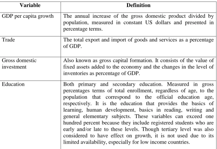
countries that differ in their income levels. Based on the convergence theory, we would expect that low and middle income countries have a higher rate of growth than the rich ones. The Gini index variable is the focal point of this paper. Therefore, it is crucially important to consider it in each area of this study. Of course other explanatory variables that are derived from growth theories might have also strong effects on growth. It is beneficial to define each variable further to facilitate and provide a complete picture of the model. In accordance with the World Bank definitions, a short description and measurements of these variables are provided in table 2.

Table 2: Variables’ definition

Variable Definition

GDP per capita growth The annual increase of the gross domestic product divided by population, measured in constant US dollars and presented in percentage terms.

Trade The total export and import of goods and services as a percentage of GDP.

Gross domestic investment

Also known as gross capital formation. It consists of the value of fixed assets added to the economy and the changes in the level of inventories as percentage of GDP.

Education Both primary and secondary education. Measured in gross percentages terms of total enrollment, regardless of age, to the population that correspond to the official education age, respectively. It is the education that provides the basics of learning, human development, basics in reading, writing and general elementary subjects. These variables can exceed one hundred percent because they include registered students who are early and/or late to these levels. Though tertiary level was also considered to have effect on growth, it is not used due to its limited availability, especially for low income countries.

5.3 Descriptive Statistics

Table 3 shows the descriptive statistics of our data, providing important information about the data variations. More complete descriptive statistics are provided in appendix 4. The maximum and minimum value ranges from negative values, as observed in the growth data, to an excess of one hundred percent as observed in the education data, which could occur as explained in table 2.

Variations can be observed if one examines the minimum and maximum value of the variables. The mean values of the data trend to be evenly between the minimum and maximum values. As such they appear to be not biased towards any end of the distribution.

(20)

Therefore it may not produce any biased results once statistical regressions and tests are performed.

Table 3: Descriptive statistics

N Minimum Maximum Mean Std. Deviation

Growth 90 -1.300336 13.37781 3.727678 2.628575 Gini Index 90 23.17850 62.32557 38.34273 9.548821 Trade 90 25.18976 277.5374 84.82184 41.36503 Capital Formation 90 10.01062 41.48055 22.45783 5.069246 Primary Education 90 12.01845 142.9345 83.33904 26.60916 Secondary Education 90 51.32259 141.5717 103.7155 11.43584 5.4 Data

The cross-sectional data consist of averaged 2002 to 2006 data for 90 countries. The data were averaged in order to overcome any minor data absence and short term fluctuations. Also, there was no major economic crisis and no major fluctuations in this particular time period that might disturb the data. These countries were not sampled but selected on the basis of the availability of at least one Gini index observation.

For this kind of macroeconomic study, a major database is required which must contain all the figures we need for the variables in our model. The World Bank database (Databank, World Development Indicators) is selected on the basis of credibility and accessibility, because it is a major global institution and collaborates with public institutions of its member-countries worldwide. Except for the Gini index data, all other variables’ data have been collected from the World Bank database. Data on countries’ Gini indices have been collected from the UNU-WIDER, a body that belongs to the United Nations.

Regarding the Gini index data there are some data limitations that are worth mentioning. These limitations might disturb the regression process and yield non-viable results. One of these limitations is the unavailability of a complete five-year Gini index data set for the majority of our selected countries. In these cases the Gini index is averaged over less than the full set of years, 2002 to 2006. In some cases only one year is used for the Gini index. This is not considered to be a major problem since the Gini index is expected to change very slowly. There is also a minor absence of education data for some countries for some years, and again simply less years are used in the averages.

(21)

5.5 Regression Results

The Ordinary Least Square (OLS) method is implemented to estimate the model. Table 4 depicts the regression results with crucial information about the variables’ coefficients and their corresponding p-values. The fitness of the data to the overall regression line is represented by R2, which indicates the variation in growth by these variables. The complete results are shown in appendix 5.

Table 4: Regression results of dependent versus independent variables2

Variable Coefficient Prob.

C -3.398982 0.1418 Gini index -0.073313 0.0211* Trade 0.004427 0.3794 Capital Formation 0.209632 0.0000** Secondary Education 0.024065 0.0324* Primary Education 0.000517 0.9787 DL 4.217618 0.0000** DM 4.152479 0.0000** R2 0.550394 F-Statistic 14.34025

Adjusted- R2 0.512013 Prob. (F-statistic) 0.000000

**Significant at 1% level *Significant at 5% level

By investigating the regression result, we observe that some of the variables are highly significant while others are highly insignificant. The coefficient of the Gini index is negative and significant at the 5% level. Therefore, it indicates a negative correlation between income inequality and growth, i.e. when Gini index increases by one percentage point the growth decreases by 0.073 percentage points.

On the other hand, the dummy variables’ coefficients are highly significant at any standard level, which match our expectation, which is based on convergence theory. The gap in output growth between the high-income countries on one side and the middle and low income countries on the other side seems to be narrowed in accordance with convergence theory. The low-income countries converge at a faster rate than the middle income as their growth rate is more than fourfold than the high. The middle-income countries grow less than that. This

2_{In order to observe how income category affects the dynamics of inequality two additional variables were}

created in our standard model by multiplying Gini index by DLi and DMi respectively. The result is presented in

appendix 6. We have omitted these two variables because they caused the Gini index coefficient to become highly insignificant.

(22)

could be the reason for the relatively higher growth rate and potential investment opportunities in the low and middle-income countries respectively.

Furthermore, at any standard level of significance, the capital formation coefficient provides a meaningful statement for the existence of the positive relationship between investment and growth. The prediction of our model regarding investment states that a 1 percentage point increase in an investment capacity of an economy at the aggregate level leads to 0.2 percentage points of growth. The emphasis on investment by the neoclassical theory seems appropriate.

At a lower degree of significance, i.e. the 5% level, the secondary education variable contributes at 0.024 percentage points to growth. But due to the insignificant value of the primary education variable and the absence of the tertiary level, the education element in our model cannot provide a complete framework of its relationship to growth. Also, the trade openness variable is highly insignificant.

5.6 Tests of the Regression

There are several statistical tests that must be performed in order to determine and ensure the validity of the estimated model. The tests are also helpful to determine if the model can be accurately used for inferential statistics and predictions.

The Variance Inflation Factor (VIF) test checks the degree to which multicollinearity might create a problem. If the correlation between explanatory variables is high, it poses several statistical problems by affecting each other’s explanatory power. Multicollinearity almost always exists in statistical regressions. However, the issue is not of its existence, but its degree. Therefore, a rule of thumb states that when the VIF is less than ten then the issue of multicollinearity is not considered to be a serious problem. Table 5 shows the VIF for each variable.

By observing the VIF we can assess the multicollinearity issue. Statistically it might not be considered to be a severe problem since the VIF is less than ten for all the variables. Attached to appendix 7 a further investigation is depicted in a correlation matrix.

Table 5: Variance Inflation Factors

Variable Centered VIF

C NA Gini 2.339361 Trade 1.133549 Capital formation 1.126414 Secondary education 2.284158 Primary education 1.288492 DL 3.307048 DM 2.114980

Also, the data must be normally distributed in order to provide accurate results, because the method implemented requires normality. Despite that the Jarque-Bera test probability,

(23)

presentation of the residuals shows similarity to a bell-shaped normal curve. Nevertheless, the non-normality indicated by the Jarque-Bera test indicates that we should be cautious regarding inference with this model.

A heteroscedasticity test was performed to determine if the OLS method is valid for our estimated model. The complete figures attached to appendix 9. Table 6 shows the results of White’s test. Based on the p-value of the chi-square, the test indicates that we cannot reject the null hypothesis of homoscedasticity. Statistically the heteroscedasticity does not appear to be a problem for inference.

Table 6: Heteroscedasticity’s White test

Obs*R-squared 32.55865 Prob. Chi-Square(32) 0.4393

In addition to these tests which provide an insight into the estimated model’s credibility and the ability for a possible accurate prediction, a test of linear function validity is required. To see whether our data fits a linear equation and if the method appropriately used, we conducted a residual plots procedure of both the Gini index and growth. The residual plots, displayed in figure 6, are derived from two regressions respectively, the Gini index and the growth against the rest of the variables. The figure displays a negative relationship between the Gini index and the growth in an otherwise non-systematic pattern. Also, it does not provide a sufficient evidence for a non-linear function relationship. Therefore, figure 6 provides additional support for the negative estimated coefficient of the Gini index in equation (1) and table 4.

Figure 6: The residual plots of the Gini and growth -4 -2 0 2 4 6 8 -15 -10 -5 0 5 10 15 20 GINI G R O W T H

(24)

5.7 Discussion

The outcomes of the empirical framework of this paper provide interesting results. The main regression results and tests, at the aggregate level, suggest a significant negative correlation between GDP per capita growth and the Gini index (inequality). The result is supported by several statistical tests procedures that make it viable and, therefore, it provides a general understanding of the issue in the global context.

The negative sign of the Gini index coefficient is contrary to the findings of the Kuznetians which indicate a positive correlation between inequality and growth. When investigating the validity of the Kuznets curve, it is essential to consider the stages of development of each country because Kuznets hypothesis considers the positive correlation in the early stages of development, i.e. during the transfer from an agricultural to an industrial economy. However, generally the negative coefficient of the Gini index considers low inequality inducive and beneficial for growth. Our finding is in line with the findings of Alesina and Rodrik (1994) and Person and Tabellini (1994), which are that high inequality is detrimental for growth. As has been mentioned in the theoretical part, Murphy, Schliefer, and Vishny (1989) also consider high inequality not inducive for growth as high inequality reduces aggregate national demand and therefore slows down the process of industrialization and economic growth. However, as Anand and Kanbur (1993) state, if different functional forms and different analytical approaches are used, different correlations could be found. Thus, despite that the main regression result of our model is in line with the conclusions of Deininger and Squire (1998), Alesina and Rodrik (1994) and Person and Tabellini (1994) which reject the notion of positive correlation between growth and inequality, another regression result on eight Latin American countries indicates a positive correlation between growth and inequality3. Interestingly, the result of the regression on these Latin American countries is in line with Kuznets stylized fact and many other researchers, notably the findings of Ahluwalia, et al. (1979) and Forbes (2000). Since most of the Latin American countries in our regression are in the early stages of development and wealth accumulation, that finding is more coherent and consistent with the Kuznets hypothesized curve, particularly with the upward sloping portion of the curve. However, as far as the number of observation in the Latin American countries’ regression is only eight and the regression has an unusually very high R2 which is 0.999698, we should be very cautious in interpreting this result and its implication.

The finding of the main regression of this paper is also in line with the previous findings on high performance Asian economies (HPAEs). These Asian economies could manage to experience high growth with low inequality, which is against conventional Kuznetsian wisdom.

While the main results of this paper regard low inequality both stimulating and beneficial for growth, one must be very cautious to generalize the findings because of the positive correlation between growth and income inequality that has been found in a number of previous studies. However, as discussed and found in many recent academic and empirical studies on developing countries, unless certain policies, such as government direct transfer, improvements in education, are in place, growth alone cannot decrease inequality after certain point. Berg and Ostry (2011) point out that these developing countries cannot sustain their growth unless they bring the level of inequality down, because growth is robustly associated

(25)

with low inequality. This supports our result at the aggregate level, which considers low inequality inducive and beneficial for growth.

Actually, the mechanical study of the correlation between growth and inequality is not the right way and approach to find the effect of growth on inequality or vice versa. Growth is a variable that might affect inequality, but there are many other factors, such as institutions, geographical location, land reform, education, form of government, etc. that can affect growth and inequality simultaneously either in a positive or negative way.

The ambiguity of the issue requires further research and a new framework that must include different factors and actors in the field. Growth alone cannot explain the causes and consequences of inequality or low inequality, and inequality or low inequality is not the only factor that policy makers must consider when looking for growth stimulating policies. The complexity and the contradictory nature of the issue require those other economic, social, political, historical, and even cultural factors to be considered when studying and analyzing the relationship between growth and inequality.

For the sake of more convincing, viable and accurate results, inequality should be studied at a microeconomic level in relationship with other microeconomic variables, along with growth, because per capita income growth cannot explain the overall observed variations in inequality in different countries. Consequently, the relationship between growth and inequality, including the form, scale and depth of this relationship, should be treated with caution because the application of different approaches, functional forms and frameworks can produce different results and conclusions that could be conflicting and contradictory to each other as are the results of our study with the previous studies of many other researchers in the field of growth and inequality.

6. Conclusion

This paper has investigated the correlation between growth and income inequality (the Gini index) in a cross-sectional data of 90 countries from 2002 to 2006. All the variables have been averaged and the countries have been classified into three categories based on their income per capita according to the findings of figure 4: high income, middle income and low income. The Kuznets Hypothesis (also known as inverted U-shaped curve or Kuznets curve), which is a controversial economic theory, states that there is a positive correlation between growth (growth in income per capita) and inequality in the early stages of economic development and as countries accumulate more wealth and grow more, the inequality decreases over time. This paper has examined this theory and has empirically investigated if the theory is relevant. The Kuznets Hypothesis and some other economic theories on the linkage between growth and inequality are further used to analyze the empirical results of this paper.

The Gini index has been used as the main independent variable, with trade openness, capital formation, primary education, secondary education and dummies for the middle and low income countries as control variables. The main focus of the paper has been on inequality that is measured by the Gini index.

The main regression result of the paper shows a negative correlation between growth and the coefficient of the Gini index at a significant level. The negative correlation suggests that low

(26)

inequality is beneficial for growth, i.e. countries with low inequality tend to grow faster. However, as far as some previous studies found a positive correlation, we must be very cautious to jump to any conclusion, such as suggesting that high or low inequality is good for growth because of the positive or negative sign of the coefficient of the Gini index.

Furthermore, the result of the scatter plots of the Gini index versus income per capita shows that Kuznets curve is detected to a certain point.

The conflicting results of this paper and also the previous conflicting findings of others (ranging from upright “U” to inverted “U” to positive linear and negative linear) on the relationship between growth and inequality suggest that only growth and inequality variables cannot explain all the variations in inequality and/or growth from country to country. Other economic and socio-political factors and actors can affect the result profoundly.

6.1 Suggestion for Further Research

The results of this paper indicate a negative relationship between the coefficient of the Gini index and growth which is significant at any standard level. The residuals and the individual scatter plots of growth and the Gini index, despite some outliers that have been resulted to a wider distribution of the data around the fitted line, indicate a linear negative correlation between the two variables. Conversely, some previous studies on the issue found a positive correlation between growth and income inequality.

These conflicting results suggest the need for further studies on the microeconomic level that should consider the specific economic and socio-political structure and factors of each individual country or a group of countries with the more or less the same level of economic development, institutions and other socio-political factors. Historical factors (such as colonialism and land reform), a variety of economic and political institutions and legal framework are among those factors that might affect inequality and, therefore, they should be included in any further study on the issue. Time series analysis over more than 20 years might provide accurate, viable and significant empirical results on the relationship between inequality and growth.

(27)

List of References

Aghion, P. & Bolton, P. (1997). A theory of trickle-down growth and development. The Review of Economic Studies, 64(2), 151-172.

Aghion, P., Caroli, E., & Garcia-Penalosa, C. (1999). Inequality and economic growth: the perspective of the new growth theories. Journal of Economic literature, 37(4), 1615-1660. Ahluwalia, M. S. (1976). Inequality, poverty and development. Journal of development economics, 3(4), 307-342.

Ahluwalia, M. S., Carter, N. G., & Chenery, H. B. (1979). Growth and poverty in developing countries. Journal of Development Economics, 6(3), 299-341.

Alesina, A. & Rodrik, D. (1994). Distributive politics and economic growth. The Quarterly Journal of Economics, 109(2), 465-490.

Alesina, A., & Perotti, R. (1994). The political economy of growth: a critical survey of the recent literature. The World Bank Economic Review, 8(3), 351-371.

Anand, S. & Kanbur, S. R. (1993). Inequality and development A critique. Journal of Development economics, 41(1), 19-43.

Banerjee, A. V. & Newman, A. F. (1993). Occupational choice and the process of development. Journal of political economy, 101(2), 274-298.

Barro, R. J. (2000). Inequality and Growth in a Panel of Countries. Journal of economic growth, 5(1), 5-32.

Birdsall, N., Ross, D. & Sabot, R. (1995). Inequality and growth reconsidered: lessons from East Asia. The World Bank Economic Review, 9(3), 477-508.

Deininger, K. & Squire, L. (1998). New ways of looking at old issues: inequality and growth. Journal of development economics, 57(2), 259-287.

Forbes, K. J. (2000). A Reassessment of the Relationship between Inequality and Growth. American economic review, 90(4), 869-887.

Godoy, R. A., Gurven, M., Byron, E., Reyes-García, V., Keough, J., Vadez, V., ... & Pérez, E. (2004). Do markets worsen economic inequalities? Kuznets in the bush. Human Ecology, 32(3), 339-364.

Josten, S. D. & Truger, A. (2003). Inequality, Politics, and Economic Growth: Three Critical Questions on Politico-Economic Models of Growth and Distribution (No. 3). Diskussionspapier/Helmut-Schmidt-UniversitätHamburg,Fächergruppe

Volkswirtschaftslehre.

Korzeniewicz, R. P. & Moran, T. P. (2005). Theorizing the relationship between inequality and economic growth. Theory and Society, 34(3), 277-316.

(28)

Kuznets, S. (1955). Economic growth and income inequality. The American economic review, 45(1), 1-28.

Kuznets, S. (1963). Quantitative aspects of the economic growth of nations: VIII. Distribution of income by size. Economic development and cultural change, 11(2), 1-80.

Lundberg, M. & Squire, L. (2003). The simultaneous evolution of growth and inequality*. The Economic Journal, 113(487), 326-344.

Murphy, K., M. Shleifer, A. & Vishny, R. (1989). Income distribution, market size, and industrialization. The Quarterly Journal of Economics, 104(3), 537-564.

Paukert, F. (1973). Income distribution at different levels of development: a survey of evidence. International Lab. Rev., 108, 97.

Persson, T. & Tabellini, G. (1991). Is inequality harmful for growth? Theory and evidence (No. w3599). National Bureau of Economic Research.

Ray, Debraj (1998). Development Economics, Princeton, Princeton University Press.

Saez, E. & Recession, G. (2013). Striking it Richer: The Evolution of Top Incomes in the United States (Updated with 2011 estimates). University of California-Berkley working Paper, 1-8.

Data Sources

Alvaredo, Facundo, Anthony B. Atkinson, Thomas Piketty and Emmanuel Saez, The World Top Incomes Database, http://topincomes.g-mond.parisschoolofeconomics.eu/, 03/12/2013. The World Bank, Data Bank. http://databank.worldbank.org/data/home.aspx. Retrieved on 2013-10-09

United Nations University, UNU-WIDER

(29)

Appendix 1: Income data distribution

Data Source: Credit Suisse Research Institute, Global Wealth Report, October 2010.

Data Source: Congressional Budget Office, Average Federal Taxes by Income Group, “Average After-Tax Household Income,” June, 2010.

(30)

(31)

(32)

(33)

Appendix 2: The value of the Gini index for each country

Country Gini Country Gini Country Gini

Ecuador 62,3 Bahamas, The 40,7 Tajikistan 33,0

Brazil 57,5 Malaysia 40,3 Mongolia 32,8

Paraguay 56,8 Serbia 39,8 China 32,6

Panama 55,8 Uzbekistan 39,7 Lithuania 32,4

Colombia 55,3 Burkina Faso 39,5 Canada 31,9

Chile 54,6 Malawi 39,0 Korea, Rep. 31,6

Honduras 54,4 Jordan 38,8 Ireland 31,5

Bolivia 52,8 Guinea 38,6 Spain 31,3

Argentina 52,4 Iran, Islamic Rep. 38,4 Switzerland 31,1

Nicaragua 52,3 Ukraine 38,2 Pakistan 30,9

Guatemala 52,1 Japan 38,1 Australia 30,1

Peru 51,4 Portugal 38,0 Albania 29,6

Dominican Republic 51,1 Yemen, Rep. 37,7 Croatia 29,0

Mexico 50,4 India 36,8 Germany 28,3

El Salvador 50,1 Kazakhstan 36,5 Malta 28,0

Costa Rica 48,9 Kyrgyz Republic 36,4 France 27,3

Russian Federation 48,0 Estonia 36,2 Norway 27,1

Philippines 47,9 Macedonia, FYR 36,0 Luxembourg 27,0

Mozambique 47,3 Moldova 35,7 Netherlands 27,0

Nepal 47,2 Poland 35,6 Belgium 27,0

Georgia 46,6 Romania 35,3 Cyprus 27,0

Venezuela, RB 46,4 Italy 34,7 Austria 26,5

United States 46,2 Lao PDR 34,6 Slovenia 26,0

Uganda 45,7 United Kingdom 34,5 Hungary 25,7

Turkey 45,5 Egypt, Arab Rep. 34,4 Finland 25,7

Uruguay 45,5 Bulgaria 34,1 Slovak Republic 25,6

Cote d'Ivoire 44,5 Latvia 34,0 Sweden 24,6

Armenia 42,9 Greece 34,0 Denmark 24,5

Thailand 42,0 Indonesia 33,9 Iceland 24,0

The Puzzle between Economic Growth and Income Inequality