Characterizing the state of water in an amorphous magnesium carbonate using Dielectric spectroscopy

(1)

UPTEC-F 13015

Examensarbete 30 hp

Maj 2013

Characterizing the state of

water in an amorphous magnesium

carbonate using Dielectric spectroscopy

(2)

Teknisk- naturvetenskaplig fakultet UTH-enheten Besöksadress: Ångströmlaboratoriet Lägerhyddsvägen 1 Hus 4, Plan 0 Postadress: Box 536 751 21 Uppsala Telefon: 018 – 471 30 03 Telefax: 018 – 471 30 00 Hemsida: http://www.teknat.uu.se/student

Abstract

Characterizing the state of water in an amorphous

magnesium carbonate using Dielectric spectroscopy

Olle Ahlström

In the industry of today, materials which can adsorb and hold large amounts of water are playing an important role. Here, the free and bound water carrying capacity of an amorphous magnesium carbonate and how these parameters depend on the relative humidity of the surrounding environment is investigated. To do this, the technique of dielectric spectroscopy is employed. Along with the water binding properties, the concentration of charge carriers and the diffusion coefficient was determined. A smaller part of around 10-30 % of the water adsorbed was shown to behave as free water in the material. The concentration of charge carriers was calculated to be in an order of magnitude of 10^18-10^22 m-3 for the higher relative humidity

environments. The diffusion coefficient was shown to be about 5*10^-9 (m^2)/s for the adsorption spectrum which is in good agreement with the value for OH- ions in water.

ISSN: 1401-5757, UPTEC-F 13015 Examinator: Tomas Nyberg Ämnesgranskare: Maria Strømme Handledare: Isabelle Pochard

(3)

Sammanfattning

Amorfa material som kan adsorbera stora mängder vatten blir allt viktigare i dagens industri. I den här rapporten studeras ett sådant ämne som nyligen är framtaget. För detta ändamål används tekniken Dielektrisk spektroskopi. Tekniken används oftast för att beskriva inre struktur i ett material. Material som ska undersökas placeras mellan två elektroder och en växelspänning med varierande frekvens appliceras. Frekvenssvaret i form av permittivitet, impedans, konduktans etc ges som utdata vid en mätning. Dessa värden tolkas sedan med avseende på de polarisationsmekanismer som ger sig tillkänna. Huruvida, och, i vilken mängd som vatten som adsoberas i materialet binds till materialet eller upptas i materialets små porer vid olika luftfuktighet utreds här. Dessa mätningar utförs och analyseras både för adsorption och desorption eftersom de båda kurvorna väntas ge något skiftande värden vilket också visar sig vara fallet. Ytterliggare information om materialet i form av koncentration av laddningsbärare, diffusionskoefficienten undersöks även här. Materialet visar sig ha 10-30 % av det absorberade vattnet fritt och rörligt i porerna medan restrerande mängd binds direkt till materialets molekyler. Koncentrationen av laddningsbärare beräknades till omkring 1018 -1022 m-3 för de högre relativa luftfuktigheterna. Diffusionskoefficienten visade sig vara ca. 5*10-9 m2/s för adsorbtionskurvan.

(4)

1

1. Introduction

1.1 Background

Inorganic amorphous materials which adsorb and can harbor large amounts of water are important in the industry of today. The number of applications in which they prove useful us has steadily been growing in the past decade. Their usefulness range from hygiene products like skincare moisturizers1 to environment sustainability Carbon Capture and Storage devices.2 There exist several materials with similar properties to the one in the current study. An advantage of, and a promising future market for this particular amorphous magnesium carbonate is to be used for reducing humidity of air in laboratories, particularly when synthesizing medicine, a process particularly sensitive to any trace of moisture interfering. The reason for this is in part due to the capacity to adsorb high levels of moisture content at low relative humidity environments but mainly because of its low regeneration temperature which lowers the expenses for production.2 However, the full potential future

usefulness of the material on the market is yet to be discovered. 1.2 Aim of thesis

The aim of this thesis is to find several parameters of interest concerning this amorphous magnesium carbonate. In doing this, the technique of dielectric spectroscopy will be used. The first parameter that will be looked for is the way in which the water behaves inside this material, i.e. whether it is bound at the surface of the material or if it behaves as free water. A method for doing this is developed and described. Prior to, and in order to do this, an in-depth analysis of the permittivity spectrum will be done. Other parameters investigated here is the number of charge carriers and the diffusion coefficient . In order to extract these parameters it will be necessary to know the direct conductivity . Hence, calculating will forego developing a method for and performing the extraction of and .

(6)

3 2

Theory

2.1

Dielectric polarization

The dielectric spectroscopy technique makes it possible to describe the internal structure of or examine a specific property of a material by analyzing the various polarization phenomena observable in that material. Hence, in order to fully grasp the concept of the dielectric spectroscopy technique, some background knowledge on dielectric polarization comes in handy. Here, the most basic principles of polarization will be sketched.

The term polarization refers to various phenomena taking place in materials in the presence of an electric field. Dielectric polarization means the specific kind of polarization that occurs in a dielectric medium. In this section, after treating the basic principles, we will describe some specific forms of polarization phenomena that could contribute to the result of our dielectric spectroscopy measurements.

2.1.1 General description of the polarization phenomena

The theory presented in this part is previously described by Jonscher.3 When a dielectric material is placed in an electric field, a separation of charges takes place which gives rise to a polarization P:

= (2.1)

Here, is the electric susceptibility, is the permittivity in vacuum, and E is the applied electric field. The electric susceptibility indicates the degree of polarization in a dielectric material in response to an electric field.4 It makes the electric susceptibility a material-specific parameter. As polarization occurs, charged species inside the material will align in the direction of the field. As a result, an electric field opposing the external field is observable within the media thus reducing the overall electric field. The polarization phenomenon occurs both at the subatomic level (inside the atom), at the atomic level and at the molecular level. An example of polarization at the subatomic level is the electronic polarization, when the electron cloud of an atom becomes slightly displaced due to an applied electric field as in Figure 2.1. At the same time, polarization can occur at the atomic level. An example of this is ionic polarization in which a charged ion will become displaced with respect to other ions, hence giving rise to a polarization.

Figure 2.1 Electronic polarization, occurring at the subatomic level. The electron cloud becomes displaced due to an applied electric field.

Figure 2.2 Dipolar polarization occurring at the molecular level in water. As an electric field with magnitude E is applied, the water molecule aligns in the direction of the field.

(7)

4

5

A third possible level of polarization is at the molecular level. An example of molecular polarization is when dipoles change alignment due to an applied electric field as in Figure 2.2, called dipolar polarization.

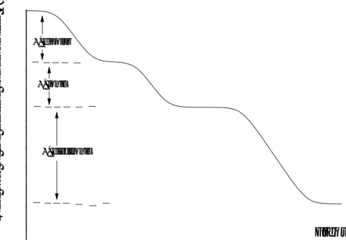
The three basic polarization mechanisms (i.e. electronic, ionic, dipole) described are present in different frequency regions.5 It can be seen in Figure 2.3. At optical frequencies, the dielectric constant arises almost entirely from the electronic polarizability. The dipolar and ionic contributions are small at high frequencies because of the inertia of the molecules and ions.5 A more in-depth description of the significance of the dielectric constant and the connection between polarization and the dielectric spectroscopy technique will be outlined in the chapter on dielectric spectroscopy.

, electronic , ionic R e a l p a rt o f th e e le ct ri c su sce p ti b ili ty,  Frequency , dipolar

Figure 2.3 Different forms of polarization mechanisms contributing to the electric susceptibility .

Polarization mechanisms that are observable with the dielectric spectroscopy technique are usually possible to describe in terms of ionic and dipolar mechanisms, the electronic mechanism being only observable by optical spectroscopy.

2.1.2 Maxwell-Wagner polarization

As a material consists of different phases, a separation of charges can take place between these phases.6 This type of polarization can be many orders of magnitude larger than to that caused by molecular fluctuations. In our case, the magnesium carbonate being investigated is amorphous, hence it has small pockets filled with air or, as it is placed in a different relative humidity, with water. This type of polarization will be visible as a steep rise in the permittivity output at approximately 10-1000 Hz range.

(8)

5 2.1.3 Electrode polarization

The theory in this part is previously described.7 Another example of separation of charges taking place is the electrode polarization. This polarization is similar to that of Maxwell-Wagner polarization in that it occurs at interfaces, but instead of the separation taking place between different phases inside the material, the electrode polarization occurs between the sample and the electrode. When a media is placed between two electrodes, as is the case in dielectric spectroscopy, mobile charge carriers (i.e. ions) are aligned towards the electrode of opposite charge. This gives rise to a capacitive effect between the electrode charges and the layer of charges in the electrolyte which decreases the overall electric field in this region. The capacitance arising from the layer of ions near the electrode can be described as

= (2.2)

where C is the capacitance per unit area, d is the separation distance between the electrode and the layer of charge in the electrolyte. As will be seen later on in this report, the electrode polarization phenomena will be visible in the dielectric spectroscopy measurement results.

2.1.4 Other polarization phenomena possibly contributing.

As water is adsorbed to a material, its polarizability can be expected to change. This is because the adsorbed water has different polarizability than the material which adsorbed it. In a nanoporous material like ours, the water molecules can either behave as free water (located in small interstices, pores inside it) or it can be bound to the surface of the material with any combination of the two states to different amounts of water being possible. To find the amount of the adsorbed water being bound to the surface of the material and the amount being free is the main objective of the current project.

Figure 1.4 Electrode polarization. Separations of charges takes place in the electrolyte and negative charges align toward the electrode surface, thus giving rise to a capacitive effect between the electrode and the electrolyte. The separation distance is d.

(9)

6

2.2 Dielectric Spectroscopy

In this part, I will do a brief explanation of the basics of dielectric spectroscopy (DS). First, a derivation of the classic Debye equations will be done. These equations are great tools in understanding the dielectric spectroscopy technique and they are also (in a slightly modified form) often useful when interpreting measurement data. The derivation of the Debye equations builds from the foundation laid in the previous section on polarization. Next, a few things will be said about how the dielectric spectroscopy technique has evolved over time. Summing up, an example of a dielectric spectroscopy measurement will conclude the chapter.

2.2.1 Derivation of the Debye equations

In this section, many concepts has been described previously.8 In Dielectric Spectroscopy, the material of interest is placed between two electrodes, a sinusodial AC-voltage rendering an electric field

= (2.3)

is applied, and the angular frequency is varied over a range of frequencies. Here, is the amplitude of the field, is the angular frequency of the field, and t is the time elapsed. This procedure causes polarization to occur inside the material. When the voltage changes sign, a de-polarization takes place and as a result, in a very short amount of time, the polarized species has returned to their original positions. Assuming that Equation (2.1) is still valid for the dynamic response, which is the case for small values of E, we define the polarizability P of the material:

= ( ) (2.4)

Here, ( ) is the frequency-dependent electric susceptibility. Assuming that the rate of change of P is always proportional to the deviation from the equilibrium value for the current applied field

= (2.5)

Here, the relaxation time is introduced. This is the time it takes for a polarized species to return to its original position. Each polarization mechanism corresponds to a certain relaxation time. Using Equation (2.5) this gives:

( ) = ( ) ( ) (2.6)

The term (0)is the susceptibility at low frequency, referred to as the static susceptibility. Restructuring gives:

( ) = ( ) = − ′ (2.7)

When using dielectric spectroscopy, there are an upper limit to the maximum frequency, in our case a range ≤ 10 MHz are being used. At higher frequencies (in the order of > 1 GHz), the contributions are hidden in a “infinity-frequency” term . We will also extend this expression to the case where we have many mechanisms contributing:

(10)

7

∗_{( ) =} _{+ ∑} ( ) _(2.8)

Splitting into real and imaginary components:

= + ∑ ( ) (2.9)

= ∑ ( ) (2.10)

These equations were first published in 1927 by Peter Debye. Hence, polarization mechanisms with this type of behavior are usually called Debye-type mechanisms. Physically, this type of behavior refers to polar molecules which are freely floating in a dielectrically inert non-polar fluid. There are therefore no restoring forces tending to impose a preferred direction, only the randomizing influence of thermal agitation.9 Although, responses resembling that of the Debye response is rarely seen in solids and almost exclusively found in some liquid crystals, the simplicity of the response makes up a good starting point for deeper understanding of the dielectric spectroscopy technique.

In Dielectric spectroscopy, instead of the susceptibility, the dielectric permittivity is generally used as output10:

( ) = {1 + − ′} = ( ) − ( ) (2.11)

The frequency-dependent dielectric permittivity ( ) indicates the resistance encountered when forming an electric field in a medium, hence it is closely related to the susceptibility (which translates into the degree of polarization in a medium due to an external field). For simplicity, the summation has been removed but of course, just as with the susceptibility, many mechanisms may be contributing to the permittivity.

As will be seen in the method part of this report, we have a special interest in the permittivity at high frequencies. The decline in permittivity due to a polarization mechanism we denote ∆ and the permittivity can then be written as: 11

( ) = + ∆ (2.12)

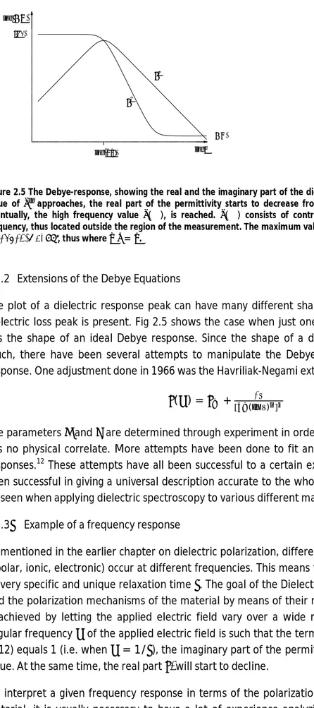
As an example, the frequency response of a material with at least one Debye-type mechanism is shown in Figure 2.5.

(11)

8 log  log '  log(1/ ' ''

Figure 2.5 The Debye-response, showing the real and the imaginary part of the dielectric permittivity. As the maximum value of approaches, the real part of the permittivity starts to decrease from the value at low frequency ′( ). Eventually, the high frequency value (∞), is reached. (∞) consists of contributions from mechanisms at higher frequency, thus located outside the region of the measurement. The maximum value of the imaginary part is reached at a frequency of 1/τ, thus where = .

2.2.2 Extensions of the Debye Equations

The plot of a dielectric response peak can have many different shapes and usually more than one dielectric loss peak is present. Fig 2.5 shows the case when just one mechanism is apparent which has the shape of an ideal Debye response. Since the shape of a dielectric response can differ so much, there have been several attempts to manipulate the Debye-equations to fit the observed response. One adjustment done in 1966 was the Havriliak-Negami extension:

( ) = + ∆

[ ( ) ] (2.13)

The parameters and are determined through experiment in order to fit the observed values and has no physical correlate. More attempts have been done to fit an even wider range of observed responses.12 These attempts have all been successful to a certain extent though none of them has been successful in giving a universal description accurate to the whole variety of responses that can be seen when applying dielectric spectroscopy to various different materials.

2.2.3 Example of a frequency response

As mentioned in the earlier chapter on dielectric polarization, different polarization mechanisms (i.e. dipolar, ionic, electronic) occur at different frequencies. This means that every mechanism will have its very specific and unique relaxation time . The goal of the Dielectric spectroscopy technique is to find the polarization mechanisms of the material by means of their respective relaxation times. This is achieved by letting the applied electric field vary over a wide range of frequencies. Once the angular frequency of the applied electric field is such that the term in the denominator of eqn (2.12) equals 1 (i.e. when = 1/ ), the imaginary part of the permittivity ′′ will have its maximum value. At the same time, the real part ′ will start to decline.

To interpret a given frequency response in terms of the polarization mechanisms taking place in a material, it is usually necessary to have a lot of experience analyzing the frequency responses of various materials.

(12)

9

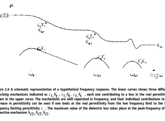
In Figure 2.6, a hypothetical dielectric is shown with three polarization mechanisms contributing to reducing the real permittivity.

Figure 2.6 A schematic representation of a hypothetical frequency response. The lower curves shows three different polarizing mechanisms indicated as ∈ " , ∈ " , ∈ " , each one contributing to a loss in the real permittivity, shown in the upper curve. The mechanisms are well separated in frequency, and their individual contributions to the decrease in permittivity can be seen if one looks at the real permittivity from the low frequency limit to the high frequency limiting permittivity ∈∞. The maximum value of the dielectric loss takes place at the peak-frequency of the

(13)

10

3. Experimental

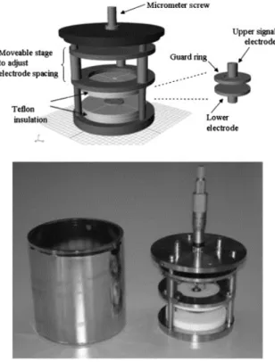
The materials used were obtained in the form of powders that had previously been synthesized by a doctoral researcher. The powders were then pressed at a pressure of 30 MPa (using a uniaxial pressing machine) to form thin, circular shaped discs of 30 mm diameter and less than 0.5 mm thick. The dielectric spectroscopy measurements were carried out using a Novocontrol Alpha-AN dielectric measurement system (Novocontrol Technologies GmbH & Co. KG). Prior to the measurements, the sample was placed in an oven at 700 C to ensure it was completely dry. The sample was placed between two gold-plated brass electrodes having a diameter of 10 mm and the electrode separation was set with a millimeter screw, Figure 3.1. The electrode arrangement was encapsulated in a stainless steel container. In the bottom of the container, a saturated salt solution was placed in order to obtain the desired relative humidity. For each desired value of the relative humidity, a specific saturated salt solution was being used. The salt solutions used were LiCl, CH3CO2K,

Mg(NO3)2, NaCl, KNO3 corresponding to 11, 23, 53, 75 and 95 % relative humidity. For the 0 %

relative humidity experiment, molecular sieves (Sigma-Aldrich, 3 Å) were placed in the bottom of the container. As with the sample, prior to the measurement, the molecular sieves were placed in an oven at 1200 C for 24 hours to dry them. The whole

arrangement was encapsulated with parafilm and stored for 24 prior to the measurement. The measurements were carried out in a frequency spectrum of 10-2-106 Hz.

Figure 3.3 Image showing the Novocontrol Alpha-AN dielectric sample holder. Reprinted with permission.

(14)

11

4. Method, results & discussion

Up until now, we have focused on the theoretical background to the Dielectric spectroscopy technique. In this part, its usefulness in solving the task at hand, which is to estimate the amount of free water in this amorphous magnesium carbonate, is developed and described. 13 Some of the physical parameters of interest such as the number of charge carriers and diffusion coefficient of the material is also calculated and discussed.

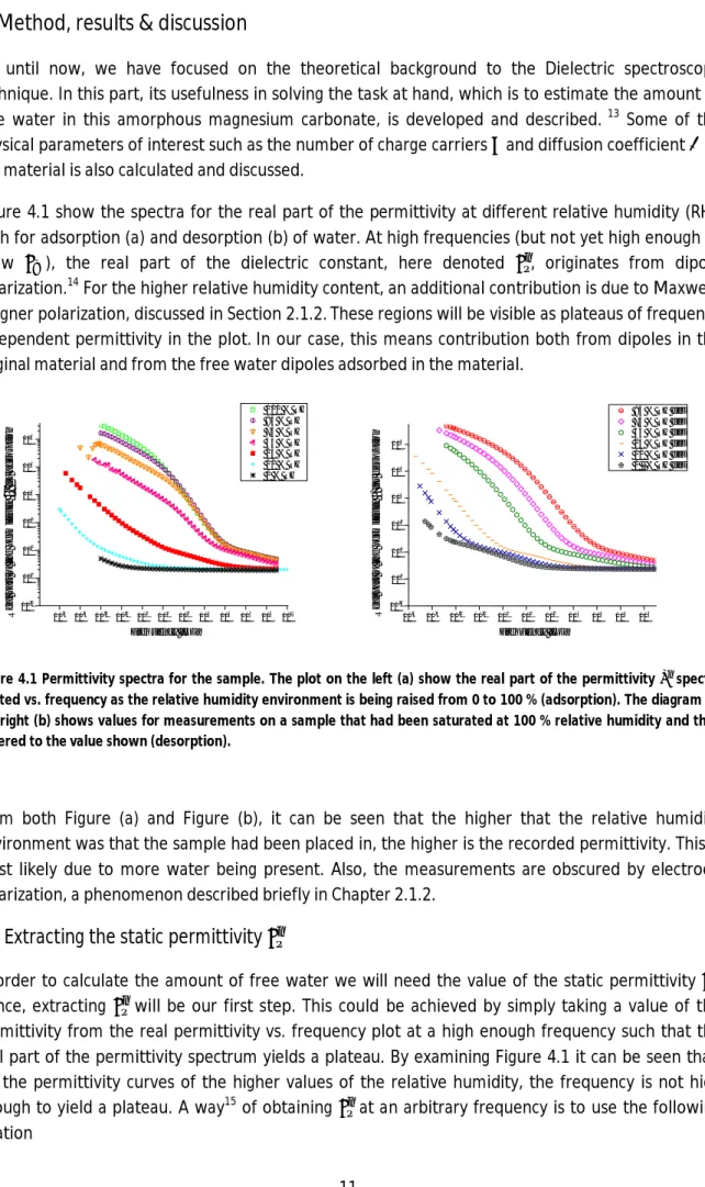
Figure 4.1 show the spectra for the real part of the permittivity at different relative humidity (RH), both for adsorption (a) and desorption (b) of water. At high frequencies (but not yet high enough to show ), the real part of the dielectric constant, here denoted , originates from dipole polarization.14 For the higher relative humidity content, an additional contribution is due to Maxwell-Wagner polarization, discussed in Section 2.1.2.These regions will be visible as plateaus of frequency independent permittivity in the plot.In our case, this means contribution both from dipoles in the original material and from the free water dipoles adsorbed in the material.

10-4 10-3 10-2 10-1 100 101 102 103 104 105 106 107 10-1 100 101 102 103 104 105 100 % RH 94 % RH 75 % RH 53 % RH 23 % RH 11 % RH 0 % RH Re a l p a rt o f th e p e rm it ti v it y ' fo r a d s o rp ti o n Frequency [Hz] 10-4 10-3 10-2 10-1 100 101 102 103 104 105 106 10-1 100 101 102 103 104 105 94 % RH des 75 % RH des 53 % RH des 23 % RH des 11 % RH des 0 % RH des R e a l p a rt o f th e p e rm it ti v it y  ' f o r d e s o rp ti o n Frequency [Hz]

Figure 4.1 Permittivity spectra for the sample. The plot on the left (a) show the real part of the permittivity spectra plotted vs. frequency as the relative humidity environment is being raised from 0 to 100 % (adsorption). The diagram on the right (b) shows values for measurements on a sample that had been saturated at 100 % relative humidity and then lowered to the value shown (desorption).

From both Figure (a) and Figure (b), it can be seen that the higher that the relative humidity environment was that the sample had been placed in, the higher is the recorded permittivity. This is most likely due to more water being present. Also, the measurements are obscured by electrode polarization, a phenomenon described briefly in Chapter 2.1.2.

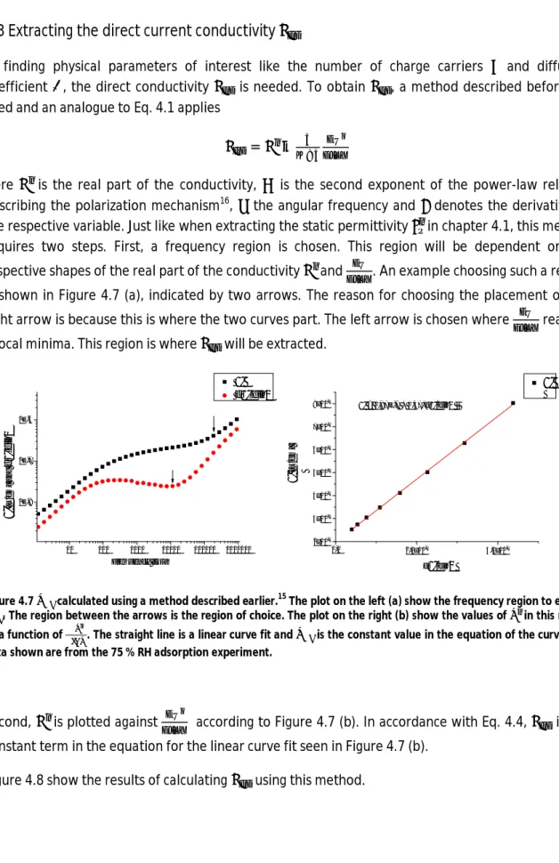
4.1 Extracting the static permittivity

In order to calculate the amount of free water we will need the value of the static permittivity . Hence, extracting will be our first step. This could be achieved by simply taking a value of the permittivity from the real permittivity vs. frequency plot at a high enough frequency such that the real part of the permittivity spectrum yields a plateau. By examining Figure 4.1 it can be seen that, for the permittivity curves of the higher values of the relative humidity, the frequency is not high enough to yield a plateau. A way15 of obtaining at an arbitrary frequency is to use the following relation

(15)

12

= − (4.1)

The variable being the exponent of the power-law relation describing the polarization mechanism16 and is the angular frequency. Here, denote the derivative of the respective variable. By plotting

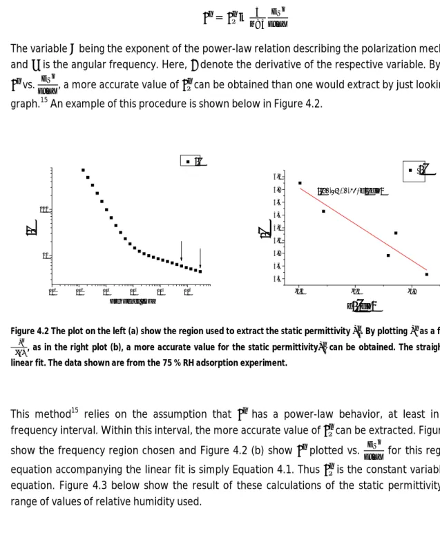
vs. , a more accurate value of can be obtained than one would extract by just looking at the graph.15 An example of this procedure is shown below in Figure 4.2.

101 102 103 104 105 106 10 100 ' ' Frequency [Hz] -1,2 -1,0 -0,8 4,4 4,6 4,8 5,0 5,2 5,4 5,6 5,8 6,0 ' 

'

d

'

/dln 'd'dln

Figure 4.2 The plot on the left (a) show the region used to extract the static permittivity . By plotting as a function of , as in the right plot (b), a more accurate value for the static permittivity can be obtained. The straight line is a linear fit. The data shown are from the 75 % RH adsorption experiment.

This method15 relies on the assumption that has a power-law behavior, at least in a small frequency interval. Within this interval, the more accurate value of can be extracted. Figure 4.2 (a) show the frequency region chosen and Figure 4.2 (b) show plotted vs. for this region. The equation accompanying the linear fit is simply Equation 4.1. Thus is the constant variable in this equation. Figure 4.3 below show the result of these calculations of the static permittivity for the range of values of relative humidity used.

(16)

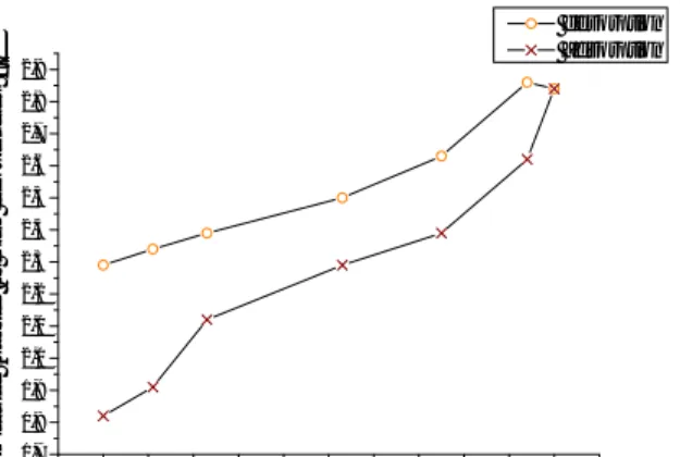
13 0 20 40 60 80 100 1,7 1,8 1,9 2,0 2,1 2,2 2,3 2,4 2,5 2,6 2,7 2,8 2,9 P e rm it ti v it y ( s ta ti c ) a t h ig h f re q u e n c ie s s ' Relative humidity % desorption adsorption

Figure 4.3 Values of the static permittivity at high frequencies as the relative humidity is increased and decreased, obtained using eq. 4.1.

Looking at Figure 4.3, the values of for the desorption spectra are higher than is the case for adsorption. The reason for this is that once the relative humidity has been raised to 100 %, thus being saturated, some part of the adsorbed water stays there even if the relative humidity is lowered. In order to completely remove all the water after saturation the sample has to be heated to approximately 700 C. A more detailed description of this phenomenon is seen in Figure 4.5 (a). As mentioned, the values obtained of the dielectric constant in Figure 4.3 are not originating solely from water dipoles free in the material but from dipoles present in the original material as well. Thus, in order to separate out the water contribution from the contribution of the material itself, some additional calculations will be necessary.

4.2 Extracting the water content

A suitable way of extracting the water content is to use the Maxwell-Garnet formula: 17

= (4.2)

Here, is the effective permittivity of the material (water included), is the permittivity of the dry material, is the permittivity of the inclusion (water in this case) and is the volume fraction of the inclusion. Water has a permittivity of 80 and the dry material 1,82. The value for the effective permittivity is, in this particular case, the same as the static permittivity shown in Figure 4.3. Hence, these values can be used in Eq. 4.2. The MG-formula is only valid when the majority component acts as a skin and is completely surrounding the other material.17 Thus, considering the fraction of water

present in our sample is expected to be relatively small, the formula is expected to be valid in the whole spectrum of values for the relative humidity examined. However, there is a lot of research articles published on how to find the dielectric constant of composite systems. For example the Bruggeman and Böttcher18 equations are both used for these kinds of calculations. In order to find the best possible equation to use in this particular case, additional research might be necessary and this is a possible shortcoming of the current work.

(17)

14

Assuming that only free water is contributing to the permittivity (bound water will not have a measureable effect), the calculated values for the volume fractions of free water are shown in Figure 4.4. 0 20 40 60 80 100 0,00 0,05 0,10 0,15 0,20 fr e e w a te r v o lu m e f ra c ti o n Relative humidity % desorption adsorption

Figure 4.4 the volume fraction of free water obtained using the Maxwell-Garnett formula Eq. 4.2

The curve in Figure 4.4 shows a similar shape to that of the static permittivity in Figure 4.3. This is because the amount of free water has a linear effect on the permittivity. As the volume fractions are small, in the range 0-0,18, the MG-formula is considered to be valid.

A Ph.D. student involved in another part of this project made a water sorption experiment in which the total amount of water molecules per gram of sample could be traced. The experiment was carried out from 0 % relative humidity up to approximately 95 % and then back to 0 %. The result is shown in Figure 4.5 (a). The relative humidity points shown are chosen to coincide with the ones for the dielectric spectroscopy analysis. Knowing the volume fraction of free water, the number of free water molecules present per gram magnesium carbonate can be estimated as

= (4.3)

Here, is the Avogadro number, is the molar mass of water and is the density of the sample (found to be 2,58 g/cm3 by my co-workers). The results from these calculations are shown in Figure 4.5 (b).

(18)

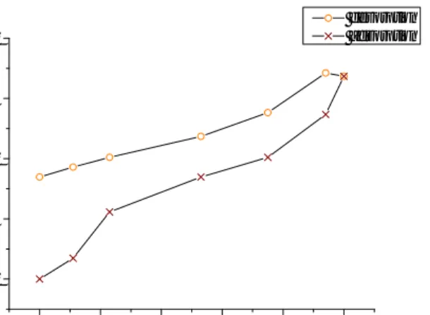
15 0 20 40 60 80 100 0,00E+000 1,00E+021 2,00E+021 3,00E+021 4,00E+021 5,00E+021 6,00E+021 7,00E+021 8,00E+021 n o f to ta l w a te r m o le c u le s p e r g ra m o f s a m p le Relative humidity % desorption adsorption 0 20 40 60 80 100 0,00E+000 1,00E+021 2,00E+021 3,00E+021 4,00E+021 5,00E+021 6,00E+021 7,00E+021 8,00E+021 n o f fr e e w a te r m o le c u le s p e r g ra m o f s a m p le Relative humidity % desorption adsorption

Figure 4.5 (a) the plot on left show the total amount of water molecules present per gram of sample. (b) The right plot shows the amount of free water molecules present per gram of sample.

As mentioned before and which can be observed in Figure 4.5 (a), the water becomes hard to remove once it has been taken up by the material. It is reasonable to assume that in the case of desorption, the path that the curve will follow on the way down will depend on the starting point for the desorption process. In other words, had we, instead of starting the desorption process from 100 % relative humidity, stopped the adsorption at 53 % RH and started desorption from there we would get different results due to a different amount of water still lingering inside the sample being hard to remove.

Comparing Figure 4.5 (a) and 4.5 (b) gives an idea about how much of the water adsorbed in the material that ends up being free to move inside rather than being bound. Figure 4.6 illustrate this more in detail. 0 20 40 60 80 100 0,06 0,08 0,10 0,12 0,14 0,16 0,18 0,20 0,22 0,24 0,26 0,28 0,30 0,32 R a ti o o f fr e e w a te r o u t o f to ta l w a te r p re s e n t in s a m p le Relative humidity % desorption adsorption

Figure 4.6 Ratio of free water out of total water present in sample.

In Figure 4.6 it can be seen that the ratio of free water out of total water is relatively small. This indicates that most of the water is directly bound to the surface of the material.

(19)

16

4.3 Extracting the direct current conductivity

In finding physical parameters of interest like the number of charge carriers and diffusion coefficient , the direct conductivity is needed. To obtain , a method described before15 is used and an analogue to Eq. 4.1 applies

= − (4.4)

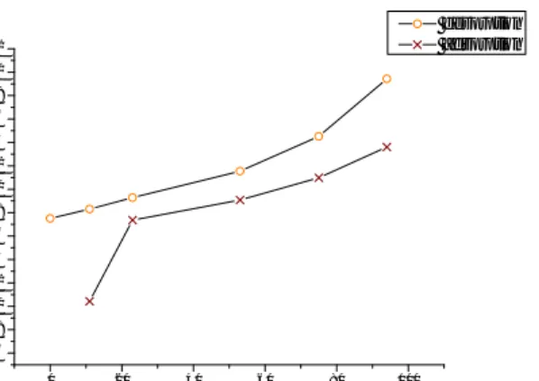
Here is the real part of the conductivity, is the second exponent of the power-law relation describing the polarization mechanism16, the angular frequency and denotes the derivative of the respective variable. Just like when extracting the static permittivity in chapter 4.1, this method requires two steps. First, a frequency region is chosen. This region will be dependent on the respective shapes of the real part of the conductivity and . An example choosing such a region is shown in Figure 4.7 (a), indicated by two arrows. The reason for choosing the placement of the right arrow is because this is where the two curves part. The left arrow is chosen where reaches a local minima. This region is where will be extracted.

10 100 1000 10000 100000 1000000 1E-8 1E-7 1E-6 ' d'dln  ' [ S /c m ] a n d d  ' d ln  Frequency [Hz] 0,0 2,0x10-7 _4,0x10-7 2x10-7 3x10-7 4x10-7 5x10-7 6x10-7 7x10-7 8x10-7 '  ' [S /c m ] d'/dln ' = 1,97E-7 + 1,37*d'/dln

Figure 4.7 calculated using a method described earlier.15 The plot on the left (a) show the frequency region to extract . The region between the arrows is the region of choice. The plot on the right (b) show the values of in this region as a function of . The straight line is a linear curve fit and is the constant value in the equation of the curve. The data shown are from the 75 % RH adsorption experiment.

Second, is plotted against according to Figure 4.7 (b). In accordance with Eq. 4.4, is the constant term in the equation for the linear curve fit seen in Figure 4.7 (b).

(20)

17 0 10 20 30 40 50 60 70 80 90 100 1E-14 1E-13 1E-12 1E-11 1E-10 1E-9 1E-8 1E-7 D ir e c t C o n d u c ti v it y d c [ S /c m ] Relative Humidity % Adsorption Desorption

Figure 4.8 the direct conductivity estimated using a method described earlier.15

The values for the direct conductivity of the adsorption spectra shown in Figure 4.8 show a steady rise with increasing water content in the sample. This is to be expected since more free water means more ions to conduct, hence higher conductivity. The error estimates make, at least in part, up for the unexpected finding that the values for the direct conductivity are higher for the adsorption spectra than for desorption. The lowest values for the adsorption curve are missing because no suitable region for extraction could be found for these points.

4.4 Extracting the number of charge carriers and the diffusion coefficient

Other physical parameters of interest are the number of charge carriers in the material as well as the diffusion coefficient .

When the frequency is high enough the electrode polarization phenomenon, described earlier in the dielectric polarization part, does not occur anymore. The reason for this is that the applied electric field changes so fast that the ions won’t have enough time to move in one direction to reach the electrode. The conductivity of this unrestricted, dc-like motion can be expressed as: 13

= (4.5)

Here, is the unit charge, is the number of charge carriers, is the Boltzmann constant and is the temperature. At lower frequencies, the movement of ions is hindered by the electrodes and thus electrode polarization occurs. The concentration of charge carriers can be calculated as13

(21)

18 =

√ (4.6)

Here, is the real part of the dielectric permittivity in the high frequency region where is dominated by dc-like ion conduction and is the angular frequency for which ( ) = . is the separation distance between the electrodes. Eq. 4.6 is only valid if the following condition is satisfied19

( )

≫ 1 (4.7)

Here, is the relaxation time.

10-3 10-2 10-1 100 101 102 103 104 1014 1015 1016 1017 1018 1019 1020 1021 1022 1023 1024 100 % RH Ads 94 % RH Ads 75 % RH Ads 53 % RH Ads 23 % RH Ads 11 % RH Ads C o n c e n tr a ti o n o f c h a rg e c a rr ie rs n [ m -3 ] Frequency [Hz]

Figure 4.9 Concentration of charge carriers as a function of frequency for adsorption. The values are calculated according to Eq. 4.6 for the adsorption spectra. For the two lowest RH values, no inflection point could be found.

(22)

19 10-3 10-2 10-1 100 101 102 103 105 106 107 108 109 1010 1011 1012 1013 1014 1015 1016 1017 1018 1019 1020 1021 1022 1023 1024 1025 1026 1027 1028 1029 1030 1031 94 % RH des 75 % RH des 53 % RH des 23 % RH des 11 % RH des 0 % RH des C o n ce n tr a ti o n o f ch a rg e c a rr ie rs n [ m -3 ] Frequency [Hz]

Figure 4.10 Concentration of charge carriers n as a function of frequency for desorption calculated according to Eq 4.6.

The values for the concentrations of ionic charge carriers in Figure 4.9 and 4.10 are rather

uncertain and, as a direct consequence, so will the values for the diffusion coefficient . The method to extract from Figures 4.9 and 4.10 is briefly discussed before in ref [13] although in our case there are no clearly defined frequency-independent regions for the extraction of the value . The reason for this is that the condition in Eq. 4.7 is not satisfied. Instead, here we use the inflection points (i.e. where the slope of the curves in Figure 4.9 and 4.10 is at a local maximum) to find . This results in the uncertainty in the extraction of that value. Especially, at the lowest relative humidity values for adsorption, no inflection points could be found.

(23)

20 0 20 40 60 80 100 1E7 1E8 1E9 1E10 1E11 1E12 1E13 1E14 1E15 1E16 1E17 1E18 1E19 1E20 1E21 1E22 1E23 C o n c e n tr a ti o n o f c h a rg e c a rr ie rs [ m -3 ] Relative humidity % desorption adsorption

Figure 4.11 charge carrier concentrations extracted at the inflection points of Figure 4.9 and 4.10.

Just as is the case for the direct conductivity, the concentration of charge carriers in Figure 4.11 shows a steady increase with the increasing amount of relative humidity, except for an unexpected jump that occurs at 23 % RH for the desorption curve. Again, this is due to the charge carrying ions that the water brings. The unexpected jump at 23% is most likely a trace of the previously mentioned inexactness of the inflection point method used here. Figure 4.12 show the values for the diffusion coefficient. The diffusion coefficient shows a fairly constant value with increasing relative humidity at about 5 ∗ 10 / for the adsorption spectrum. This is in good agreement with diffusion

coefficient for OH- ions in water. The magnesium carbonate we studied present hydroxyl groups on its surface and it is thus consistent to observe OH- as the charge carriers in the porosity of the material. The decrease of the diffusion coefficient for the desorption spectra when the relative humidity decreases could be caused by a diffusion loss due to the porosity and tortuosity of the material.

(24)

21 0 10 20 30 40 50 60 70 80 90 100 1E-20 1E-19 1E-18 1E-17 1E-16 1E-15 1E-14 1E-13 1E-12 1E-11 1E-10 1E-9 1E-8 D if fu s io n c o e ff ic ie n t D [ m 2 /s ] Relative humidity % adsorption desorption

(25)

22

5. Summary & conclusions

Dielectric spectroscopy was employed to characterize the binding properties of water and the associated charge transport mechanisms in a nanoporous material at different relative humidity environments.

This work shows that most of the water is bound to the material. A smaller amount, 10-30% of the water volume, was found to behave as free water. The amount of free water show different values for adsorption and desorption, indicating that the water is hard to remove water once it has been adsorbed. Following a topic touched upon in Chapter 4.2 of this work, one will probably see a new and different desorption curve from every starting point of the relative humidity. To do additional measurements like this is beyond the scope of this work. Knowing the amount of water that still remains inside the material as the relative humidity environment is shifted in a different direction at different values for the relative humidity could be of interest in applications of this amorphous magnesium oxide. If so, this is a possible topic for future research.

The direct conductivity and the concentration of charge carriers were found to increase with increasing relative humidity. The increases in these values were explained by the increase in the amount of free water.

The amount of free and bound water in this magnesium carbonate is known without any specific knowledge on these particular water bonds. For usage in the biotechnological area, it would be interest to know what the surface bindings for the bound water looks like. This is another topic for the future.

Acknowledgements

I would like to thank my supervisor, Isabelle Pochard, for all the great help and for always taking time to give me insight and advice throughout the course of this project. I wouldn’t have come far without her feedback. I also want to thank my reviewer Maria Strømme for all the help and for giving me the chance to work in her department. In addition I would like to thank Sara Frykstrand and the other co-workers at the Department of functional materials and nanotechnology , Ångström laboratory Uppsala, for being helpful whenever I needed it.

References

[1] Strietzel C, Svensson L. Marknadsstudie ”Uppsalit”

[2] Aulin B, Lundberg N, Nystrand M. En kommersialiseringsstrategi för ett nytt nanoporöst material [3] A.K. Jonscher, Dielectric relaxation in solids, Chelsea, London, 1983.

(26)

23 [4] Encyclopædia Britannica

[5] Charles Kittel, Introduction to solid state physics, Berkeley, California, 2005, p.464

[6] Kramer F, Schönhals A. (eds.): Broadband Dielectric Spectroscopy. Berlin, Heidelberg. Springer Verlag p. 87

[7] In: Barsoukov Y, MacDonald JR, editors. Impedance Spectroscopy, p. 63-66. 2nd ed. New York: Wiley; 2005

[8] Jan Lagerwall : Video tutorial on dielectric spectroscopy on liquid crystals, part 3 & 4 (January 2013): http://www.exicone.com/Exicone/Tutorial_download.html

[9] A.K. Jonscher, Dielectric relaxation in solids, Chelsea, London, 1983. P. 23 [10] A.K. Jonscher, Dielectric relaxation in solids, Chelsea, London, 1983. P. 46 [11] A.K. Jonscher, Dielectric relaxation in solids, Chelsea, London, 1983. P. 96

[12] A.K. Jonscher, Dielectric relaxation in solids, Chelsea, London, 1983. Chapter 8: “The many body universal model of dielectric relaxation”, p.310-363

[13] Gelin K, Bodin A, Gatenholm P, Mihranyan A, Edwards K, Strömme M. Polymer 48 (2007): 7623-7631

[14] In: Barsoukov Y, MacDonald JR, editors. Impedance Spectroscopy, 2nd ed. New York: Wiley; 2005 [15] M. Strømme Mattsson, G.A. Niklasson, K. Forsgren, A. Hårsta, J. Of applied physics Vol 84, No 4. 1999

[16] A.K. Jonscher, Dielectric relaxation in solids, Chelsea, London, 1983.

[17] Choy, Tuck C. (1999). Effective medium theory. Oxford: Clarendon Press. P. 8.

[18] H. Looyenga. Dielectric constants of heterogeneous mixtures. Physica 31 (1965) 401-406 [19] T.M.W.J. Bandara, M.A.K.L. Dissanayake, I. Albinsson , B.-E. Mellander.Solid State Ionics 189 (2011) 63–68