WARPLAM DSS: using Cluster Analysis as an approach to delineate
IWRM regions
Ana Carolina Coelho Maran, Darrell Fontane, Evan Vlachos, John Labadie, and Benedito Braga1
Civil and Environmental Engineering Department, Colorado State University
Abstract. The lack of uniform and integrated water resources regions is a critical issue, especially
in transboundary water regions and federative countries. Overlaying levels of planning and man-agement, as a result of uncoordinated water resources regions, hamper Integrated Water Resources Management. In order to harmonize multiple objectives and better represent the interaction be-tween environmental, socio-economic, political and historical aspects, it becomes imperative to de-fine appropriate territorial limits for water resources planning and management. The present study introduces an approach to support the process of delineating water resources regions. It is based both on recognition of more comprehensive aspects and incorporation of those aspects into a deci-sion support system. This paper describes how cluster analysis is applied in the model design. Dy-namic Programming is selected as the suitable method to be combined with Cluster Analysis to im-prove the algorithm efficiency.
Key Terms: water resources planning and management, decision support systems, cluster analysis, dynamic programming
1. Introduction
The lack of uniform and integrated water resources regions is a critical issue, especially in transboundary water regions and federative countries (Matthews and Germain 2007; Ganoulis et. al. 1996; EC 2002). Overlaying levels of planning and management, as a re-sult of uncoordinated water resources regions, hampers Integrated Water Resources Man-agement (IWRM). In addition, the process of delineating these regions has often been exe-cuted without sufficient scientific support, usually resulting from political and historical circumstances. In spite of this, it is possible to improve results by using knowledge from prior experiences, modern techniques and decision support systems (DSS). In order to harmonize multiple objectives and better represent the interaction between environmental, socio-economic, political and historical aspects, it becomes imperative to define appropri-ate territorial limits for wappropri-ater resources planning and management.
The present study introduces an approach to support the process of delineating water resources regions based both on recognition of more comprehensive aspects and incorpora-tion of those aspects into a DSS. The proposed Water Resources Planning and Manage-ment Regions (WARPLAM) DSS is designed to be used by federal and state governManage-ments, international commissions and water councils. Considering that river basins are the most suitable boundaries to attain IWRM goals (Dourojeanni et. al 2002; Wegerich 2008;
1
Water Resources Planning and Management Civil Engineering Department
Colorado State University Fort Collins, CO 80523-1372 Tel: (970) 491-1470
Falkenmark 2004), the DSS simulation model offers the option for decision makers to in-clude socio-economic, political and environmental aspects into the analysis, as suggested by Porto & Porto (2008). It intends to promote a better understanding about the reasoning related to this process, and to reinforce the principles of IWRM. WARPLAM DSS is also a very flexible solution to support the delineation of regions in multiple levels of subsidiarity and to be adaptable to regional circumstances.
This paper describes how cluster analysis is applied in the model design, combined with Dynamic Programming. Among the available techniques, Dynamic Programming has proven to be a valuable tool to support cluster analysis (Belman, 1973). It increases sub-stantially the algorithm efficiency, considering the number of combinations in an exhaus-tive enumeration search can be too extensive.
This paper is organized in two main topics. The first topic describes how the DSS is developed, including a general overview of its structure and procedures. The second topic is the description of the algorithm that constitutes the model of the DSS. It includes the logic associated with combining Cluster Analysis and Dynamic Programming. Finally, conclusions and general recommendations are presented.
2. WARPLAM DSS: The Proposed Approach
Water Resources Planning and Management Regions Decision Support System is the proposed approach to address the issue of lack of uniform and integrated water resources regions. It constitutes a structured and instructive tool to help decision makers to delineate water resources regions, which is usually an ill structured task. Another important charac-teristic of the proposed approach is its ability to help harmonizing multiple interests from different stakeholders.
To describe the process of developing this approach, it is helpful to understand the main steps of the decision making process related to the exercise of delineating water re-sources planning and management regions. In this study, it is organized into five basic steps. The first step it the definition of a consistent basis over which to develop an aggrega-tion process. This is a very important step because it represents the main aspect to be con-sidered for the water resources regions. From the grouping of those smaller territorial units, for example natural drainage areas or municipalities, water resources planning and man-agement regions will be created. The second step is the selection of criteria, beyond river basin boundaries, that reflect the main aspects related to IWRM principles. Those criteria represent the recognition of more comprehensive objectives and multiple interests into the analysis. A specific comparative analysis was performed, based on selected examples from European and American countries, in order to enhance the selection of criteria. This com-parative study constitutes an Expert System, as proposed by Turban (1998), used to sup-port the decision making process. This step also includes weights assignment for each cri-terion. The third step is the combination of selected criteria with the basis in order to define the ‘measure of closeness’ for each adjacent pair of territorial units contained in the basis. Each of those pairs constitutes one grouping alternative. The ‘measurement of closeness’ for each alternative is defined taking into account overlaying area values of all the criteria. The fourth step is the application of compromise programming to sum up all weighted cri-teria values for each alternative, considering the different scale range or space dimensions of the criteria’ values. The fifth and last proposed step is the application of Cluster Analy-sis to define different grouping alternatives that represent ‘ideal’ IWRM regions.
After considering the main steps of the decision making process, the DSS procedures and structure are presented, followed by a description of its components, as well as the model outline.
2.1. DSS Procedures and Structure
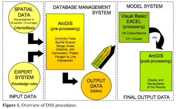
WARPLAM DSS is structured using ESRI ArcGIS, Microsoft Excel and Visual Basic functionalities. The main procedures performed within the DSS are described below.
The first two steps of the decision making process are supported mainly by ArcGIS functionalities. The criteria and basis selection is facilitated through the use of GIS tech-niques. The Expert System is integrated to the GIS interface to provide the necessary un-derstanding about the criteria selection process, based on heuristic rules derived from the comparative study. In such cases, the decision makers are able to learn from past experi-ences and to decide, based on their own preferexperi-ences, which of those aspects are important in the specific context of the case in analysis.
As described before, the basis contains the territorial units to be grouped. For example, the adoption of a consistent basis considering natural drainage area limits represents the consideration of watershed boundaries as the basis for the analysis. Instead, the adoption of municipalities represents the consideration of political-administrative boundaries as the ba-sis for the analyba-sis. The selected criteria should reflect the main aspects related to IWRM. These criteria, as well as the basis, must be available in the format of spatial data, as the necessary input for the model. As soon as the criteria are selected, data can be easily im-ported to the DSS. The ESRI Geodatabase format is recommended, but data may also be imported using shapefile or coverage formats.
After data is imported, the Database Management System handles all pre-processing analysis, as part of Step 3 of the decision making process, in order to prepare the input data to the model system. Knowledge rules, imported from the Expert System are directly inte-grated into the database. The intersection among chosen criteria and the consistent basis is performed. In order to support the creation of a more functional and user-friendly interface, the Model Builder ArcGIS functionality is used. This tool allows all the repeated tasks, to be performed at one click, according to the selected functionalities. In such case, the calcu-lation of all overlaying areas is performed by one click and the results are being incorpo-rated into the model system through the use of a single workspace. Microsoft Visual Basic functionalities are also used in this stage of the process to perform some necessary data management tasks, in integration with ArcGIS. As a result of this pre-processing stage, all overlaying areas of selected criteria are calculated and combined with the knowledge rules from the Expert System. In addition, all adjacent pairs are listed as possible alternatives to be grouped. Therefore, the necessary input for the model system is ready and the algorithm can be started.
Steps 4 and 5 of the decision making process are basically performed inside the model system, which will be described in the following section. The algorithm is developed using Microsoft Excel Macros and Visual Basic Codes, which guarantee the necessary integra-tion among the data management system and the model system. In addiintegra-tion, optimizaintegra-tion techniques are applied to support the clustering process and to increase the algorithm’s ef-ficiency. As soon as the data is read in the model system, the user needs to define the weights for each criterion and some parameters for the cluster analysis. This is also
facili-tated though a user-friendly interface. Finally, the results from the simulation are displayed into the GIS interface automatically. Figure 1 illustrates a summary of those procedures.
Figure 1. Overview of DSS procedures.
3. Model Outline and Algorithm Structure
The model structure is comprised of the algorithm developed to address the delineation of water resources regions. It is divided in two main modules, correspondent to the Steps 4 and 5 of the decision making process, as described above. The main input for the algorithm comes from the intersection between selected criteria and the basis, performed in Step 3. Each pair of adjacent units contained in the basis constitutes one alternative to be consid-ered for the cluster analysis.
Cluster analysis is a set of procedures used to create classification and reorganize data into homogeneous groups (MOPU 1984; Kaufman & Rousseeuw 1990). The first stage of the Cluster Analysis is to define a numerical measure of homogeneity (Bellman 1973; Ald-enderfer & Blashfield 1984). For that measure, this approach employs the concept of ‘measure of closeness’. It is defined, for each adjacent pair, taking into account the criteria overlaying area values over the basis. Considering that the calculations are performed based on area values, it is not necessary to standardize the data. As soon as the initial units are defined in the database management system, uniform outputs are provided. In addition, the compromise programming step handles different data dimensions. According to Coelho et. al. (2005) the ‘measure of closeness’ can be calculated through the size and proportion of the common criteria area overlaying one adjacent pair of the basis’ territorial units. Be-sides showing how relevant a common criterion is to the pair (size), the measure also needs to express how equal the two units are in reference to the criteria (proportion). In addition the common perimeter is also considered. By grouping these three aspects, the following vector-based equation was applied for each alternative and each criterion:
Ci1,2= 2 * CP1,2 PWS1+ PWS 2* AC1WS1 AWS1 * AC1WS 2 AWS 2 (1)
Considering:
ACi WS1 = Overlaying Area of Criteria i over territorial unit WS1 (i = 1, 2, …, N)
ACi WS2 = Overlaying Area of Criteria i over territorial unit WS2 (i = 1, 2, …, N)
N = number of criteria defined by the user AWS1 = Area of territorial unit WS1
PWS1 = Perimeter of territorial unit WS1
CP1,2 = Common Perimeter between territorial units 1 and 2
Ci1,2 = Measure of closeness between units 1 and 2, considering Criteria i
Ci1,2 ranges from 0 to 1
As soon as the list of alternatives (adjacent pairs) and respective measures of closeness is ready, the algorithm is started. The first module of the algorithm is the application of compromise programming to sum up the measures of closeness of each criterion value for each alternative, resulting in the total measure of closeness Ca,b for each alternative. This method was considered the most adequate considering the different scale range of criteria values (different space dimensions) and its ability to rank alternatives according to their ‘closeness’ to certain ‘ideal’ criteria levels (Hajkowicz & Collins 2007; Labadie 2007). The scaling function was applied by the selection of the best and worst values of the alter-natives for each criterion, according to Equation 02. The Total Measure of Closeness is as-signed as a ‘link’ between adjacent basis’ territorial units, and represents the proximity be-tween those units into each pair. Compromise solutions are the result of combining differ-ent L1, L2 and L∞ norms and differdiffer-ent sets of weights.
(2)
The second module of the algorithm is the application of Cluster Analysis over alterna-tives to define different grouping alternaalterna-tives or clusters. The total measure of closeness between each pair is used as the input to the similarity matrix of elements to be clustered. It is considered the most adequate method to directly represent the relative distances be-tween the elements to be clustered. Alternatives of groups with higher similarity will be formed in order to delineate the “ideal” regions for water resources planning and manage-ment. The partitioning method is applied according to the calculated overall proximity of each cluster created. The partitioning clustering method, in contrast to the hierarchical method, generally results in better patterns of similarities between elements of the groups, because the overall distance of the group is being considered (Kaufman & Rousseeuw 1990; Aldenderfer & Blashfield 1984). This overall distance is calculated using the aver-age proximity between all elements of the group. The objective function is to maximize the overall proximity of all clusters (minimize intra-cluster variance). The constraints associ-ated with the problem are derived from the knowledge rules existent at the Expert System, according to the decision maker preferences.
A significant drawback of this method is the infinite number of alternatives to be ana-lyzed (Kaufman & Rousseeuw 1990). Depending on the number of elements to be grouped, the analysis may become too extensive. In such case, Dynamic Programming (DP) can be applied to support the evaluation of multiple alternatives. It speeds up the analysis consistently and is ideally suited to be applied with cluster analysis (Bellman 1973; Esogbue 1986).
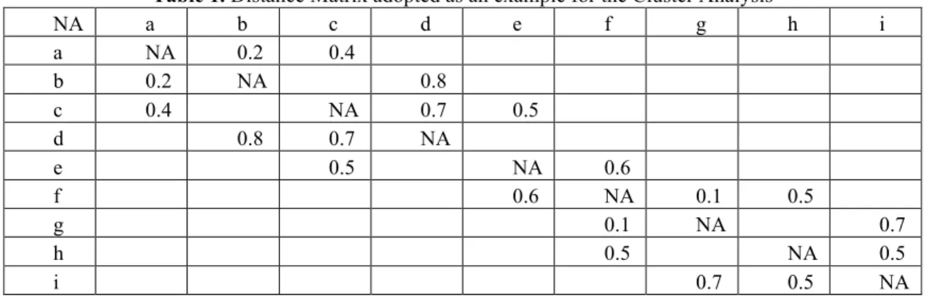
Currently, the DP method is being tested to support the analysis, using the generalized dynamic programming software developed by Labadie (1990). A 9-element data set is adopted as the trial exercise of the method in study, assuming that it is a result of the Steps 1, 2 and 3 of the decision making process. The following distance matrix contains the ‘total measure of closeness’ for each of the ten pairs of alternatives in the analysis (Table 1):
Table 1. Distance Matrix adopted as an example for the Cluster Analysis
NA a b c d e f g h i a NA 0.2 0.4 b 0.2 NA 0.8 c 0.4 NA 0.7 0.5 d 0.8 0.7 NA e 0.5 NA 0.6 f 0.6 NA 0.1 0.5 g 0.1 NA 0.7 h 0.5 NA 0.5 i 0.7 0.5 NA
The intra-cluster measure of homogeneity is calculated considering the overall average of the ‘measures of closeness’. For example, for the 4-element cluster ‘a-b-c-d’ it is equal to 0.525, taking into account the list of pairs and respective ‘measure of closeness’ con-tained in Table 2. The inter-cluster measure of homogeneity is then calculated by taking the average of the intra-cluster measure of homogeneity. For example, the nine available elements can be clustered in three groups of 2, 3 and 4 elements, respectively. The inter-cluster measure of homogeneity is then the average of the three intra-inter-cluster measures of homogeneity, as shown in Table 3.
Table 2. Intra-Cluster Measure of Homogeneity
ab 0.2
ac 0.4 Sum Average
bd 0.8 2.1 0.525
cd 0.7
Table 3. Inter-Cluster Measure of Homogeneity
ab 0.2
ac 0.4 Sum Average abcd
bd 0.8 2.1 0.525
cd 0.7
ef 0.6 Sum Average efg Sum Average
fg 0.1 0.7 0.35 0.875 0.292
hi 0.3 - - hi
It is assumed that if the cluster has one element, the intra-cluster measure of homoge-neity is equal to zero. The objective is to reduce the inter-cluster measure of homogehomoge-neity if there are clusters containing just one element. This way, the best grouping alternatives –
or the ones containing the highest inter-cluster measure of homogeneity – are more homo-geneous. For example: having clusters ‘e-f’ and ‘c-d’ (Inter-Cluster = 0.65, as the average of 0.6 and 0.7) is better than having clusters ‘c-d-e’ and ‘f’ (Inter-Cluster = 0.30, as the average of 0.60 and 0.00).
Therefore, the objective is to maximize the inter-cluster measure of homogeneity. For that, the DP analysis is divided in two parts, according to the method suggested by Bell-man & Zadeh (1970), BellBell-man (1973), Esogbue (1986). It consists in dividing the set of al-ternatives into I groups, according to the intra-cluster measure of homogeneity (measure of closeness), and determining the optimal value of I according to the inter-cluster measure of homogeneity, and then the optimal subdivision. The additive objective function is to maximize the total benefits of allocating mi objects to I clusters. The DP recursion relation
and other related equations are defined as following:
Fi(mi+1) = max [fi*(mi-mi-1) + Fi-1(mi)} (03)
Different than ui-1*(mi-1)
S.T.
0 <= xi <= M
0 < mi = xi – xi+1 <= M (no cluster with 0 elements)
mi = 1,2, …, M
For all discrete xi+1: 0 <= xi+1 <= M-i
Over stages i = 1, 2, …, M
x1 = M; xM = 0 (all element should be clustered at the end)
Optimal solution can be found in any stage when xi+1= 0
Starting with: F0(m1) = 0
Maxi Fi(M)
Considering:
M = total number of elements to be grouped mi = number of elements in the cluster
ui *(mi) = best benefit of having mi elements in the cluster
i = number of clusters = number of stages in DP xi = state variables
mi = decision variables
The decision variable is the number of elements to be included in the cluster in each stage. The state variables are the number of elements remaining to be allocated, using the concept of the resources allocation problem. They are both integer values, according to the nature of the problem. The benefit is equal to the intra-cluster measure of homogeneity (average of the measures of closeness). It is calculated in a poptimization step that re-turns the best possible benefit for a cluster having mi elements. The forward DP recursion
relation and the inverted form of the state dynamic equation are adopted.
The important concept that is added to Belman’s first proposed recursion relation is the ability to store the information calculated in the stage before and use it as an input for the sequence of the solution. The proposed method stores the best results in each stage to be used in the next stage in order to exclude the elements already clustered.
To do that, the binary string concept is also applied. This is a really efficient and unique way to organize the data. Considering all possible combinations among the ele-ments, the position in a string determines if the element is included in the cluster or not. Therefore, in each stage and state variable, the algorithm returns a unique number that is associated with a string that represents the clustered elements. There is a unique number associated with each possible combination (Table 4). This unique number is used to guar-antee that the elements previously clustered are not included in the current stage.
Table 4. Unique Number and Binary String for Different Combinations
b 128 0 1 0 0 0 0 0 0 0
c-d 96 0 0 1 1 0 0 0 0 0
c-d-e 224 0 1 1 1 0 0 0 0 0
c-e-f 88 0 0 1 0 1 1 0 0 0
c-e-f-h 90 0 0 1 0 1 1 0 1 0
In addition, the running average concept, as defined by Lee & Labadie (2007) is ap-plied to calculate the objective function in each stage. The additive objective function, in principle, does not allow the calculation of the inter-cluster measure of homogeneity in each stage, because the average is required. To overcome this issue, a discount factor (DF) is added to both parts of the recursion equation. In the first part of the recursion equation – fi*(mi-mi-1) – the discount factor is equal to ‘1/i’. In the second part of the recursion
equa-tion - Fi-1(mi) – the discount factor is equal to ‘(i-1)/i'. As a result, the objective function is
adapted to the DP format and the ‘running average’ is calculated in each stage. CSUDP al-lows the user to define a Discount Factor for the objective function. The discount factor cannot be the same for all stages because the elements would have a different weight de-pending on the stage it is selected to be part of the cluster. The DP recursion relation, in-cluding the DFs, becomes:
Fi(mi+1) = max [(1/i)fi*(mi-mi-1) + ((i-1)/i)Fi-1(mi)} (4)
It can also be observed that it is not necessary to run all the stages of the DP formula-tion because the ‘best’ soluformula-tion is not located at the end. Considering that the optimal solu-tion can be found in any stage when xi+1= 0, it is possible to check for a peak of the best
possible solutions, according to figure 2. Therefore, it is possible to stop the algorithm when the return values are below the peak, in order to increase its efficiency. To get the feedback policies for the best result, it is then necessary to run the DP again for the respec-tive stage.
4. Conclusions and Recommendations
The presented approach constitutes a prototype of a decision support system to address the necessity of defining water resources regions. As demonstrated in this paper, it includes human intuition and judgment, e.g. subjective criteria selection and weighting processes. Through a user-end focus, it also provides easy access to information; interaction, which is supported by visualization of criteria; and flexibility, since it is open to aggregate other cri-teria in order to consider new aspects. In addition, it constitutes a learning process because decision makers can better understand the aspects related to water units delineation, using Expert Systems.
Regarding the potential results, it is possible to observe that the model can easily in-corporate a set of criteria and weights. Multiple simulations can be simply performed in order to support the decision making process. Dynamic Programming has proven to in-crease the efficiency of the algorithm, especially when compared to the alternative exhaus-tive enumeration method. According to the results of the simulations being tested, for a data set containing five elements, 24 intra-cluster and 48 inter-cluster measure of homoge-neity can be found in exhaustive enumeration. Dynamic Programming one-dimensional al-gorithm analyzes only 16. For the given 9-elements dataset presented in this paper, 90 in-tra-cluster and 1300+ inter-cluster valid measures of homogeneity can be found in exhaus-tive enumeration Dynamic Programming one-dimensional algorithm analyzes around 240.
Figure 2. Possible Solutions and Respective Return Values in each stage.
Table 5 presents the maximum benefit considering the best solution for the given 9-element data set adopted as the trial exercise of the method in study.
Table 5. Maximum Benefit representing the best solution for given data set
Clusters fi(mi) mi Xi Xi+1
b-d 0.8 2 9 7
g-i 0.7 5 7 5
a-c-e-f-h 0.5 2 5 0
Max 0.67 3 clusters
The optimization of the best number of groups can be incorporated into the analysis, according to the user preferences. However, it is important to highlight the objective of this DSS is not to guarantee the optimum number of groups. Instead, different simulations of grouping alternatives seem to be more important for the decision maker in order to evalu-ate the problem.
Regarding the cluster analysis method, its key is to define ‘real groups’ instead of ‘im-posed groups’ (Aldenderfer & Blashfield 1984). In this case, the combination of cluster analysis with dynamic programming and the adopted ‘closeness measure’ guarantees ‘ideal’ solutions. The combination of these techniques used to address the presented issue is the innovation proposed in this study. However, it is important to affirm that this paper refers to an ongoing study that may lead to future reviews and adjustments.
It is expected that the final algorithm to be developed will incorporate fuzzy analysis in order to indicate the membership function of each element to its final cluster, as suggested by Kaufman & Rousseeuw (1990). It will represent the uncertainty associated with defin-ing element X as part of cluster Y. Accorddefin-ing to Hajkowicz & Collins (2007) the fuzzy set theory is excellent to handle uncertainty inherent in ill-structured problems. In addition, another advantage of the selected partitioning method for the cluster analysis is that it al-lows the representation of the results considering fuzzy logic.
In addition, it is possible that a multi-dynamic program analysis will be necessary to prove that the best solution is reached in DP. As an ongoing research project, some tests are being generated in order to evaluate it. Generic algorithm will also be assessed as a way to increase the algorithm’s efficiency. Another important aspect that needs special at-tention is the occurrence of ties when returning the benefit value, in the pre-optimization step.
Finally, the 2nd United Nations World Water Development Report: “Water, a shared responsibility” pointed out the need for an integrated and holistic approach to water re-sources management, highlighting the benefits from IWRM: 1) multiple uses and coopera-tion between different sectors; 2) coordinated management and development of land, water and other resources; and 3) balanced social, environmental and economic benefits (UNESCO, 2006). Therefore, to integrate political divisions within river basin units is one of the biggest challenges. Still according to this report, the difficulties of IWRM are di-rectly related to the fact that political boundaries are not coincident with natural river ba-sins units.
In this sense, the presented study reinforces the importance of defining IWRM units and demonstrates the DSS approach as a method to support multiple interest decision process, re-flecting human judgment through easy access to information, education, interaction and flexibility. As demonstrated, it addresses the solution of such a complex and ill-structured problem. Future decisions related to water resources regions delineation may have increased quality by using knowledge from prior experience and modern techniques, instead of letting the process to be a result of political and historical circumstances only.
References
Aldenderfer M S, Blashfield R K (1984) Cluster Analysis. Bervely Hills: Sage Publications.
Bellman R (1973) A Note on Cluster Analysis and Dynamic Programming. Mathematical Biosciences 18: 311-312p.
Bellman R, Zadeh L A (1970) Decision Making in a Fuzzy Environment. Management Science. Application Series 17(4): B141-B164p.
Coelho A C P, Gontijo W, Cardoso A (2005) Unidades de Planejamento e Gestão de Recursos Hídricos: uma proposta metodológica. In: Anais 7º Simpósio de Hidráulica e Recursos Hídricos dos Países de Língua Oficial Portuguesa – Silusba, Portugal.
Dourojeanni A, Jouravlel A, Chavez G (2002) Gestión del agua a nivel de cuencas: teoría y práctica. CEPAL Division de Recursos Naturales e Infraestructura. Serie Recursos Naturales e Infraestructura. Nr 47. San-tiago do Chile.
EC European Commission (2002) Common Strategy on the Implementation of the Water Framework Direc-tive. Project 2.9: Best Practices in River Basin Management Planning. Version:1.1 Date: August 2002. Esogbue A O (1986) Optimal Clustering of Fuzzy Data via Fuzzy Dynamic Programming. Fuzzy Sets and
Systems 18: 283-298p.
Falkenmark M (2004) Towards Integrated Catchment Management: Opening the paradigm locks between hydrology, ecology and policy-making. International Journal of Water Resources Development 20(3): 275-282p.
Ganoulis J, Duckstein L, Literathy P, Bogardi I (1996) Transboundary Water Resources Management: Insti-tutional and Engineering Approaches. NATO ASI Series, v.7. Germany: Springer.
Hajkowicz S, Collins K (2007) A Review of Multiple Criteria Analysis for Water Resource Planning and Management. Water Resources Management 21: 1553-1566p.
Jansky L, Sklarew D M, Uitto J I (2005) Enhancing Public Participation and Governance in Water Resources Management. In: Jansky L, Uitto J I, Enhancing Participation and Governance in Water Resources Man-agement – Conventional Approaches and Information Technology. Water Resouces ManMan-agement and Policy. United Nations University Press.
Kaufman L, Rousseeuw P J (1990) Finding Groups in Data: an introduction to cluster analysis. Wiley Series in Probability and Mathematical Statistics. New York: John Wiley & Sons, Inc.
Labadie J W (2007) Lecture Notes. Seminar on Engineering Decision Support and Expert Systems – CIVE610. Colorado State University, Fort Collins, Colorado.
Labadie J W (1990) Dynamic Programming with the microcomputer. In: KENT A, WILLIANS J (eds.) En-cyclopedia of Microcomputers. V.5. New York, NY: Marcel Dekker, Inc. 275-338p.
Lee J H, Labadie J W (2007) Stochastic optimization of multireservoir systems via reinforcement learning. Water Resources Research 43, W11408.
Matthews O P, Germain D S (2007) Boundaries and Transboundary Water Conflicts. Journal of Water Re-sources Planning and Management. 133(5):386-396p.
MOPU Ministerio de Obras Públicas y Urbanismo da España (1984) III Técnicas para el tratamiento de la in-formación, in: Guía para elaboración de estudios del medio físico: contenido y metodología. Centro de Estudios de Ordenación Del Territorio y Medio Ambiente, 507-569p.
Porto M F A, Porto R L (2008) Gestao de Bacias Hidrograficas. Estudos Avancados 22(63) 43-60p.
Turban E (1998) Decision Support and expert systems: management support systems. 4ed. Englewood Cliffs, New Jersey: Prentice-Hall Inc.
UNESCO (2006) The 2nd United Nations World Water Development Report: ‘Water, a shared responsibil-ity’. Available at: http://www.unesco.org/water/wwap/wwdr2/
Wegerich K (2008) Shifing to Hydrological Boundaries: the politics of implementation in the lower Amu Darya basin. Physics and Chemistry of the Earth. In press, correct proof.