Quality Control of Light Emitting Diodes : Using power factor, harmonic distortion and light to power ratios

(1)

16019

Examensarbete 15 hp

Juli 2016

Quality Control of Light Emitting

Diodes

Using power factor, harmonic distortion

and light to power ratios

Aksel Wännström

(2)

Teknisk- naturvetenskaplig fakultet UTH-enheten Besöksadress: Ångströmlaboratoriet Lägerhyddsvägen 1 Hus 4, Plan 0 Postadress: Box 536 751 21 Uppsala Telefon: 018 – 471 30 03 Telefax: 018 – 471 30 00 Hemsida: http://www.teknat.uu.se/student

Abstract

Quality Control of Light Emitting Diodes

Aksel Wännström; Abdirahman Mohamed

This study addresses quality control for Light Emitting Diodes (LED) according to fouraspects, the power factor of LED lamps, their harmonics and total harmonic distortion (THD), the luminosity for total power to radiated power ratio.

It focuses on four brands and six different LED lamps, and concludes that IKEA's LED lamps pertain as the quality lamp, with a power factor over 0.9, THD less than 4% and a power to radiated light of over 4%.

ISSN: 1401-5757, TVE16019 Examinator: Martin Sjödin Ämnesgranskare: Viviana Lopes Handledare: Uwe Zimmermann

(3)

Populärvetenskaplig Sammanfattning

Ljusdiod-lampor eller LED-lampor är en relativt ny metod att belysa hemmet med men tekniken har funnits för kommersiellt bruk sedan 60-talet. Den första ljusdioden som släpptes för kommersiellt bruk var rödfärgad men genom åren har färgerna blå och grön framkommit och genom en blandning av dessa har det blivit möjligt att få lamporna att lysa vitt. Detta har resulterat investering och utveckling av LED-lampan som ett alternativ till den existerande glödLED-lampan. LED-lampor antas ha en energiförbrukning som är flera gånger lägre än andra lamp-alternativ, men dem påstås också att dem smutsat ner elnätet med frekvenser som är annorlunda än elnätsets 50 hertz. Vårt mål är att utforska dessa påståenden och dessutom ta fram slutgiltiga resultat angåande vilken LED lampa som har bäst kvalite.

(5)

1 Introduction

Light Emitting Diode (LED) lamps are continuously increasing in popularity. They are substituting out most lamps in the modern area in most house holds and general electronics. The reason? They are energy saving due to low energy consumption and have an increased durability compared to their counterpart lamps. They differ from normal halogen and incandescent lamps as they produce a unique wave-spectrum depending upon the LED construction and emit photons in the specifics wavelength of the visible frequency. Continuing from an environmental aspect, they are practically free of any toxic substance such as mercury and lead compared to incandescent and fluorescent lamps. Previous research shows that LED lamps exhibit said features there are still some concerns for LED lamps; Mentioning aspects such as overtone harmonics on the electrical net with a potential for disturbance in electrical circuits.1 LED lamps actual power usage to run their drivers. Forcing energy companies to increase their production of energy without any monetary benefits as the power is "unused".2This project presents several aspects of LED lamps quality that are studied and measured; first, the overtones subjected to the network are calculated from the current. Second, the power factor of LED lamps from the root-mean-square method (rms) of current and the rms of voltage, Third, the light intensity from LED lamps from the light spectrum and lastly its intensity at various wavelength. All of these aspects are compared for 6 LED lamps and a Halogen lamp as a control lamp. The goal with the project is to test the quality of a variety of LED lights, and compare light bulbs from different manufacturers and different properties with each other. Areas to control are the properties stated from the manufacturers, as well as stress testing and quality control of individual components within the LED lamps themselves, and if the lamps perform according the the EU legislation. An attempt at building a LED lamp fulfilling the property requirements and surpassing the tested lamps. 1.1 Harmonics

Harmonics are frequently mentioned throughout the circuit and electronic sector these days but they have existed since the first alternating current (AC)-generator was put online. Today it is seen as a growing problem since more products that cause harmonics are connected to the electric net and more electronic products are more sensitive to these small disturbances.1.

Harmonics are described mathematical as f = n ∗ ffundemental where n=1 is the fundamental

fre-quency, n=2 is first harmonic, n=3 is the second harmonics etc.

The main cause of harmonics in the electric power system is the presence of non-linear loads, like LED-bulbs and batteries to name a few. Linear load means if current that is drawn is sinusoidal while non linear load means if the current that is drawn is non sinusoidal after sinusoidal ac-voltage was giving. Capacitive,inductive and resistive loads are examples of linear load.

Figure 1. Linear and Non-linear load3

Non-linear load its a growing problem for the electrical distribution system because its generates currents with different frequency from the distribution frequency which is around 50 hertz.

(6)

If the current that drains the system is non-sinusoidal, the harmonics can disturb the distribution system in the multiple ways such as but not limited to overheating transformer, increasing the current drain and energy looses.

Figure2is an example of a non-linear load combined resultant wave of the first and thirds harmonics4.

Figure 2. First, Third and Resultant Harmonics

1.1.1 Tripled Harmonics

A look at how the non-linear load is affecting the electrical system; It is known that various multiples of the harmonic frequency are potentially more damaging than other multiples. These are known as triple harmonics and are defined as the odd multiples of the third harmonics5(ex 3rd, 9th, 15th, 21st etc.)

Neutral conductors on 3-phase systems are known to be vulnerable for tripled harmonics since they are additive compare to fundemental frequency and even harmonics. These loads from the tripled harmonics can cause a break on the conductors insulator which can cause fire hazard.5

1.1.2 Fast Fourier Method

Fourier analysis of a periodic function is made up of a series of sines and cosines functions that, when superposition, gives us a reproduced function of the original function. This new function is called the Fourier series. The fast Fourier transform is a mathematical method that transforms a function of time into a function on the frequency domain. It is made for fast computing of the discrete Fourier transform (DFT) and is useful for analyzing a time-dependent phenomena6.

An example is the study of physical phenomena such as the alternating electrical current which may be periodic in character7.

1.2 Power factor

The power factor for DC-current is P=IV where p is the power measured in watts, I is the current measured in ampere and V is the voltage measured in volts. This is also applied for AC-current when it comes to instantaneous power. However, the average power in a AC-current is made by terms of root mean squared (rms) voltage and current with additional term called the power factor8.

The power factor is a cosinus term where the angle phi is the angle between the voltage and current. Power factor can described us cos(phi)=R/Z where R is the resistances and Z=impedance but it also can be described us fraction between real power (rp) and apparent power (ap) through cos(phi)=rp/ap

(7)

The Figure2describes the relation between real, apparent and reactive power2. They are in turn related to the power factor since the fraction between real power (rp) and apparent power (ap) gives us the power factor.

Figure 3. Real, Apparent and Reactive Power

The AC-current is most effective when the actual power usage is equivalent to the apparent power; this means that we have a power factor of one, which is the most beneficial, if the actual power usage is not equivalent to the apparent power usage we have a "loss" of power somewhere, this is called the reactive power, and then we have a power factor that is less than 1 which is not beneficial to the electrical companies as more power is needed than what is being used by the device.

2 Methods

2.1 Material and Equipment:

• 1 x Portable research spectrometer (Li-1800)

• 6 x LED-lamps : Ikea: 1000, 60; LEDSAVERS: 400, 470; Anslut:470; Biltema: 470; • 1 x Halogen Lamp 30 watt

• 2 x Stand Clamps with pole allotments • 1 x Stand

• 3 x metal poles • 1 x pole clamp • 1 x light socket

• 1 x computer with VGA input • 1 x VGA cable

• 2 x rulers • 3 x cable ties

(8)

• 1 x oscilloscope

• 1 x current clamp meter • 3 x banana cables

Software Requirements of Computer:

Program for communication with Spectrometer : (PuTTY) Program for calibrating the produced files : MATLAB

2.2 Intensity of Wavelengths of LED Lamps

Using a spectrometer. Light intensity is measured per w/m over a span of wavelengths ranging from 300nm to 1100nm for a diverse collection of LED-lamps in a controlled environment.

Measurements from 300 nm to 1100 nm as this encompasses the visible light spectrum.

Calculation of the intensity for the wavelength spectrum

1. Initialize the Li800 Spectrometer as shown in Appendix A.0 2. Initialize the Log in PuTTY as shown in Appendix B

3. Set up equipment as shown in diagram4and diagram5. 4. Attach LED lamp at socket point.

5. Adjust Spectrometer to another spot following a circular motion.

6. Send commands to the spectrometer to start measuring using PuTTY interface as shown in Appendix A.1

7. Show data from PuTTY using commands shown in Appendix A.2 8. Save Data Using PuTTY interface following instructions in Appendix B

9. Measure using length measurement equipment (rulers in our case) the length, height, and hypotenuse from the spectrometer to the center of the LED lamps.

10. Repeat steps 3-9 for all the positions of interest.

(9)

Figure 4. Spectrometer and light bulb setup

Figure 5. Spectrometer and computer setup Importing Data to Matlab

1. Calibrating from Li1800 to text values in MATLAB. 2. Use MATLAB code, import from csv

3. Run calibration code cal_li1800.mat 4. Save *text*_cal file

5. Do steps 1-4 for all lamps

Voltage and Current of Lamps

Use an oscilloscope. The current and voltage for the power factor and the total harmonic distortion. 1. Attach the current reader cord to the oscilloscope and lamp current as in diagram5

(10)

2. Set the lamp as in Diagram4

3. adjust readings to account for several periods

4. Use the oscilloscope to save the values of the lamp. See appendix C for instructions on oscilloscope usage.

5. Repeat steps 1-4 for all Lamps.

3 Results

The following section presents the results from the three aspects of this study. First the total light intensity, luminosity for LED lamps and the most efficient power to light conversion. The second section shows the power factor and the LED-lamp with the greatest power factor. Last, the harmonics and total harmonic distortion where the LED lamp with the lowest distortion has the best quality.

3.1 Light Spectrum and Light Luminosity

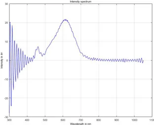
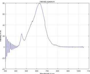
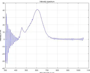
Led-lamps described as ”warm-white” where chosen to this study. Comparing the light spectrum of graphs 6 7 8 9 10 11and 12 it can be seen that there are two peaks for all LED lamps whereas the halogen lamp increases with the increase in wavelength for all measurements. Peaks of all LED lamps coincide with 450nm and 600nm with the 600nm having the greater intensity. These wavelengths correspond to blue LED diodes and yellow LED diodes respectively. Hence LED lamps emit light only at specific wavelengths.

To obtain the overall power for each LED lamp, integrate across the light spectrum for all measured points. Linearize a plot for the integrated points on a sphere and integrate again for the total area of the sphere. (MATLAB code can be seen in Appendix D) The intensities powers are listed in table1.The lamp producing the most light power is the halogen lamp, but the most efficient converting of power to light is the LED-lamp Ikea1000.

(11)

Figure 7. Biltema’s intensity per wavelength from 300nm to 1100nm

(12)

Figure 9. IKEA 60 lumens per Watt LED lamp’s intensity per wavelength from 300nm to 1100nm

(13)

Figure 11. Ledsaver 470 lumens LED lamp’s intensity per wavelength from 300nm to 1100nm

Figure 12. Halogen lamp’s intensity per wavelength from 300nm to 1100nm

Table 1. Power converted to light compared to actual power usage

Brands Actual Power (µW ) Watt Used (W) Radiated Power (W) Lumens per Watt (lm/W)

Ledsaver400 1.1827 ∗ 105 3.6 0.033 111 Ledsaver 470 2.1232 ∗ 105 7 0.030 67 Ikea1000 5.2998 ∗ 105 13 0.041 77 Ikea60 2.8535 ∗ 105 10 0.029 6 Biltema 1.0889 ∗ 105 4.2 0.026 112 Anslut 2.4548 ∗ 105 6.5 0.038 72 Halogen 1.0244 ∗ 106 30 0.034 14

(14)

3.2 Power Factor

The power factor is measured to know how effective an appliance is, and can be used to compare the amount of power used by a device to do work(real power) to the amount of power needed to actually run the device (apparent power).There is an overall standard on the power factor allowed within LED Lamps and according to the EU LED quality charter the power factor needs to be a minimum of at least 0.5 to be allowed for sale and usage by corporations. For the experiment we determined the power factor of 6 LED lamps compared to a control Halogen lamp which is a pure resistance lamp and therefore has a power factor of 1 by default.

The power factors are presented in Table 2 and it can be seen that there is some error of measurement as the halogen lamp has a power factor of less than 1. Furthermore there is a great spread in the power factor for the LED lamps themselves with some being below the EU standard, note the Biltema and the Ledsaver 400 and some being almost on par with the Halogen Lamp, namely the IKEA series, both registering a power factor above 0.9, the best out of all the various LED lamps.

Table 2. Power Factor of Various Brands Brands Power Factor Ledsaver 400 0.4062 Ledsaver 470 0.8073 Ikea 1000 0.921 Ikea 60 0.944 Biltema 0.418 Anslut 0.745 Halogen 0.996 3.3 Harmonics

By examining the FFT of the returning current it is possible to see the dimensions of all the harmonics for the LED lamps, It is also possible from these values calculate the Total Harmonic Distortion (THD)9. It is calculated as T HDf =

√

I₂2+I₃2+I₄2+I₅2...

I1 , which is the percentage disturbance that the harmonics affect the

system. It is the ratio of the total sum of the rms of all harmonics compared to the fundamental harmonic. It gives a measure of how the LED lamps affect the electric net. In figures13,14,15,16,17,18and19 the fundamental frequency and its harmonics are shown. As expected for figure19, the Harmonics are near zero and a low THD as shown in table3. The greatest THD reaching near 200% is the Ledsaver 400 and the most efficient are the Ikea 1000 and the Ikea 60.

(15)

Figure 13. Ikea’s 1000 lumens LED lamps harmonics

(16)

Figure 15. Biltema’s LED lamp’s harmonics

(17)

Figure 17. Ledsavers 470 lumens LED lamp’s harmonics

(18)

Figure 19. Halogen lamp’s harmonics

Table 3. The Total Harmonic Distortion for the Various LEDs

Brands THD Ledsaver 400 2.091 Ledsaver 470 0.493 Ikea 1000 0.182 Ikea 60 0.116 Biltema 0.606 Anslut 0.634 Halogen 0.026

(19)

4 Discussion

The study shows the IKEA LED lamps consistently are of the most favorable considering the criteria. The greatest power to light ratio of 4% of total power going in being converted to light, the largest power factor at 0.944 and with a THD barely above the 0.1 percentile make . Though it may use a third of the watt of our control halogen lamp (30W) at 13W, which would mean it is more costly for the average consumer compared to the Ledsavers 400 lumens LED lamp at 3,4W. It will still be recommended LED lamp from this study as it has the greatest efficiency, and best power factor performance, and the lowest disturbance from harmonics. All LED lamps had Harmonic distortion, as well as a power factor less than one.

5 Conclusion

For the tested LED lamps the IKEA series have the best quality defined by power factor, overtones, and power to light ratio.

To further expand upon this study there are two possible routes, use a wider variety of LED lamps and brands to include a more general market view and percentage followed by having several trials on a specific brand using many lamps of the same kind to check the quality from from lamps within the same brand. Another modification to this study could be stricter criteria for the quality, an increase in points, for example, including the driver construction, how it transforms from AC-current to DC-current, the components and their quality.

A study made by Jettanasen & Pothisarn10 suggest that the driver construction can be improved by connecting a low-pass filter to reduce the total harmonic distortion and make the outcome current more sinussoidal.

(20)

References

1. Sankaran, C. Effects of harmonics on power systems (1999). URL http://ecmweb.com/ power-quality/effects-harmonics-power-systems. Accessed June 2016.

2. Orange & Rockland. Real, apparent, reactive power (2016). URL http://www.oru.com/ images/content_images/reactivepowernew.gif.

3. Studebaker, P. When Power Quality Eats Into Energy

Effi-ciency (2016). URL http://www.sustainableplant.com/2011/

when-power-quality-eats-into-energy-efficiency/?show=all. Accessed June 2016.

4. Reinhausen. First, third and resultant harmonics (2016). URLhttp://www.reinhausen.com/ desktopdefault.aspx/tabid-1528/1847_read-4669/.

5. Micheals, K. Fundamentals of harmonics (1999). URL http://ecmweb.com/content/ fundamentals-harmonics. Accessed June 2016.

6. Nave, C. R. Fast fourier method (1998). URLhttp://hyperphysics.phy-astr.gsu.edu/ hbase/math/fft.html. Accessed June 2016.

7. Britannica, E. Harmonic analysis. Britannica Academic (2016). URLhttp://academic.eb. com.ezproxy.its.uu.se/EBchecked/topic/255491/harmonic-analysis.

8. Nave, C. R. Power factor (1998). URL http://hyperphysics.phy-astr.gsu.edu/ hbase/electric/powfac.html. Accessed June 2016.

9. Csanyi, E. Essential basics of total harmonic distortion (thd)

(2015). URL http://electrical-engineering-portal.com/

essential-basics-of-total-harmonic-distortion-thd. Accessed June 2016. 10. Jettanasen, Chaiyan and Pothisarn, Chaichan. Analytical study of harmonics issued from led lamp

driver (2014). URLhttp://www.iaeng.org/publication/IMECS2014/IMECS2014_ pp683-686.pdf. Accessed June 2016.

(21)

Appendix

Appendix A explains the three various stages for the Spectrometer LI1800 that we used for our experiment; Appendix A.0 explains how to initialize the spectrometer for our needs. Appendix A.1 explains how to start a scan with the spectrometer. Appendix A.2 explains how to transfer that scan to the PuTTY terminal before it is saved in a readable log file.

Appendix A.0

Initializing the Spectrometer

Li1800 response User input Comment

FCT: // Asking for a Function

WA // Wait Time

OLD: 1000ms NEW:

0 “Enter” //Wait Time = 0 : Press “Enter”

FCT: //Asking for a Function

SY //Synchronize Gratings

Appendix A.1

Starting A New Measurement:

Li1800 response User Input Comment

SC // Scan

FILE: //Asking for a Function

*** ”Enter” // *** = name of file : Press “Enter”

REM: //optional comment

“Enter” // : Press “Enter”

LO: //Lower Frequency Limit

300 “Enter” //300nm minimum wavelength

HI: //Higher Frequency Limit

1100 “Enter” //1100nm maximum wavelength

# Scans //Asking for Number of scans

“Enter” //Can enter a number: we only want one scan which is default

(22)

Appendix A.2

Transferring The Measurement

Li1800 response User Input Comment

SH “Enter” //Show Data in PuTTY : Press “Enter”

S,A,W: //Asking for display

S “Enter” //Serie Display in PuTTY : Press “Enter” FILE:

*** “Enter” //*** = name of saved file : Press “Enter” LO: 300 “Enter” // HI: 1100 “Enter” // INT: “Enter” // LABEL: “Enter” Appendix B

Appendix B explains how to save log files using the PuTTY terminal with some pictures for guidelines. To allow the system to save the files from the spectrometer there are several steps that need to be done in PuTTY: Before any scans are conducted create a log for saving the data in: This is done by right clicking on the PuTTY icon in the upper left hand corner of the terminal window as seen in Figure20. Selecting Change settings and going to Logging under Sessions as seen in21and22of appendix B. Here click the browse button and at the location of where you want to save the file enter the name for your next scan as shown in figure23and figure24. You are now ready to log the next scan from the spectrometer.

(23)

Figure 21. Saving from Putty Step 2

(24)

Appendix C: Oscilloscope Instructions to save graphs as data points Insert Portable Harddrive / USB, in usb port.

Click Option button; Click Save image; Enter Name; Click Save to USB;

(25)

Appendix D: MATLAB code for integrating across the surface area of a sphere from 5 defined points with wavelength measurements

name1 = input(’InsertFile name, e.g. Anslut470 : ’,’s’) ; name = [name1, ’.txt’]; x=dlmread(name,”,[0,0,4,0]); y=dlmread(name,”,[0,1,4,1]); r= sqrt(x.2+ y.2) + eps; phi=atan(y./x); phi2 = linspace(min(phi),pi/2,100); z=cos(phi2);

name= [name1,01cal.txt0];

M1 = dlmread(name,”,[1,1,376,1]); V1 = dlmread(name,”,[1,0,376,0]); p1=trapz(V1,M1);

M3 = dlmread(name’,”,[1,1,376,1]); V3 = dlmread(name,”,[1,0,376,0]); p3=trapz(V3,M3);

name= [name1,05cal.txt0]

M5 = dlmread(name,”,[1,1,376,1]); V5 = dlmread(name,”,[1,0,376,0]); p5=trapz(V5,M5); p=[p5 p4 p3 p2 p1]; if y(1) < y(2) p = fliplr(p); end p2 = zeros(1,100); p2 = interp1(phi,p,phi2); plot(phi,p,’o’,phi,p) hold;

title(’Graph of the intensity through different angles’) xlabel(0Anglesinradians[cm2]0) ylabel(0Intensity[uW /cm2]0) vikt = z.*p2; plot(phi2,p2,’o’,phi2,p2) plot(phi2,vikt,’x’,phi2,p2) ints = trapz(phi2,vikt.*)

(26)

Appendix E: MATLAB code for calculating the power factor using the rms of current and voltage

%Plotting The power factor from Oscilloscope

%Need to create a file called Tid.mat which contains a matrix which covers %the time spectrum

%Prompt is for already pre-loaded files for Lamps. Must already be in the %workspace.

%Change this to match the variable name needed;

tiden = load(’Tid.mat’); %The Period of time for which the measurement is taken tid = tiden.Tid;

name = input(’InsertFile name, e.g. Biltema470 : ’); %loads the file with the measured current of the LAMP

PowerGrid = zeros(2000,2);

%Justiyfing for the shift in time due to measurment error PowerGrid(1:1990,2) = name(11:2000,3);

PowerGrid(1:2000,1) = name(1:2000,2); PFact= zeros(2000,1);

PFact = PowerGrid(1:2000,1) .* PowerGrid(1:2000,2); PFact2 = sum(PFact(1:2000))/1990;

%taking the RMS for the necesarry factors

rms = sum(PowerGrid(1:2000,1).*PowerGrid(1:2000,1)); rms = rms/2000; rms = sqrt(rms); rmsi = sum(PowerGrid(1:2000,2).*PowerGrid(1:2000,2)); rmsi = rmsi/1990; rmsi = sqrt(rmsi);

%calculating the power factor powerfactor = PFact2 / (rms*rmsi)

(27)

Appendix F: MATLAB code for finding the FFT and the Harmonics name = input(’Choose a File for FFT Add : ’,’s’);

name1 = [name, ’.mat’]; load(name); Abil = load(name1); var3 = fields(Abil); name2 = Abil.(var31); x = name2(1:2000,2); %x = dlmread(name,”,[0,1,2000,2]); %x = (1:2000,3); m = 2000; n = m; fs = 100000; dt = 1/fs; t = (0:m-1)/fs; y = fft(x); amp = abs(y/m); power = amp(1:m/2+1); P1 = power; P1(2:end-1) = 2*P1(2:end-1); f reinc= f s ∗ (0 : (m/2))/m; fig1 = figure; plot( f re_inc, P1); hold saveas(fig1,[’v’,name,’2’],’jpeg’); peaks = findpeaks(P1); C = peaks > 0.004; val = peaks(C); A = val(2:size(val)); thd = sqrt(sum(A.*A))/val(1)