Mobile Satellite Communications: Channel Characterization and Simulation

MEE 07:14

Mobile Satellite Communications

(Channel Characterization and Simulation)

Ajayi Taiwo Seun

This thesis is presented as part of Degree of Master of Science in Electrical Engineering

Blekinge Institute of Technology

May 2007

Blekinge Institute of Technology School of Engineering

Department of Applied Signal Process & Telecommunications Supervisor: Dr. Abbas Mohammed

-Abstract

The channel characterization of a mobile satellite communication which is an important and fast growing arm of wireless communication plays an important role in the transmission of information through a propagation medium from the transmitter to the receiver with minimum barest error rate putting into consideration the channel impairments of different geographical locations like urban, suburban, rural and hilly.

The information transmitted from satellite to mobile terminals suffers amplitude attenuation and phase variation which is caused by multipath fading and signal shadowing effects of the environment. These channel impairments are commonly described by three fading phenomena which are Rayleigh fading, Racian fading and Log-normal fading which characterizes signal propagation in different environments. They are mixed in different proportions by different researchers to form a model to describe a particular channel.

In the thesis, the general overview of mobile satellite is conducted including the classification of satellite by orbits, the channel impairments, the advantages of mobile satellite communication over terrestrial. Some of the major existing statistical models used in describing different type of channels are looked into and the best out of them which is Lutz model [6] is implemented.

By simulating the Lutz model which described all possible type of environments into two states which represent non-shadowed or LOS and shadowed or NLOS conditions, shows that the BER is predominantly affected by shadowing factor.

-Acknowledgement

First and foremost, I would to thank my advisor and supervisor, Docent Abbas Mohammed, at Blekinge Institute of Technology for giving me the opportunity to work with him and for all his efforts, patience and his encouragement toward the successful completion of this thesis.

Also, I have to express my profound gratitude to Maria Solomonsson of Applied Signal Processing Department for the counsel and advice given to me during this research thesis work, I just want to say thank you for all your time you spare for me.

I would like to thank all my colleagues in the department, especially my friends who have contributed to the success of this work in one way or the other. I want you to know that I appreciate you and God bless you all.

Last but not the least, a special thank you to my darling wife who has stood by my side all these while making sure that the thesis is successful. I love you sweetheart.

Ajayi Taiwo Seun Karlskrona, May 2007

-Table of Contents

Abstract ... v

Acknowledgement ...vii

List of Figure and Tables...xii

Short List of Abbreviations ... xv

Chapter 1 ... 1

Introduction ... 1

1.1

Aim and Objectives ...2

1.2

Literature Review ...2

1.2.1

Classification of mobile satellite communication. ...2

1.2.2

Frequency Bands ...8

1.2.3

Benefits of mobile satellite system over terrestrial system...9

1.2.4

Thesis structure...9

Chapter 2 ...11

Propagation Channel Impairments...11

2.1

Introduction ...12

2.2

Basic Propagation Mechanisms ...12

2.3

The impairments ...14

2.4

Types of Fading ...20

2.4.1

Fading Based on Multipath Delay Spread ...20

2.4.2

Fading Based on Doppler Spread ...21

Chapter 3 ...23

Statistical Models ...23

3.1

Introduction ...24

3.2

The Basic Probability Distribution Functions...25

x

-3.3

The Major Channel models...28

3.3.1

Loo’s Model...29

3.3.2

Corazza’s Model...29

3.3.3

Lutz’s Model...30

3.3.4

Nakagami’s Model ...31

3.3.5

Norton’s Model...31

Chapter 4 ...33

Implementation of Lutz’s Model ...33

4.1

Introduction ...34

4.2

Generation of Statistical Distributions ...34

4.2.1

Generation of Rayleigh/Rician data set...34

4.2.2

Generation of Lognormal data set ...35

4.2.3

Generation of Shadowed data set ...36

4.2.4

Generation of Unshadowed data set ...36

4.2.5

Generation of Total data set...37

4.2.6

Propagation Model Parameter for Typical LMSS...37

Chapter 5 ...39

Results and Conclusion ...39

5.1

Simulation Results ...40

5.2

Bit Error Rate ...47

5.3

Conclusion...49

xii

-List of Figures and Tables

Figure 1.1

Elevation and Coverage angles...3

Figure 1.2

Different Types of satellite Orbits ...6

Figure 2.1 Three Basic Propagation Mechanisms: Reflection, Deffraction

and Scattering ...13

Figure 2.2

Constructive and Destructive Addition of Transmission Paths ....14

Figure 2.3

Fading As 2 Incoming Signals Combine with different Phases ...15

Figure 2.4

Two Pulses in Time-Variant Multipath...15

Figure 2.5 Illustration of Shadowing and Refraction ...16

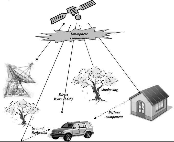
Figure 3.1

Mobile Satellite Propagation Environment...24

Figure 5.1

Generation of Lognormal data set & the PDF (25% Shadowing) 41

Figure 5.2

Generation of Rayleigh data set and the PDF (25% Shadowing).41

Figure 5.3

Generation of Unshadowed (Rician) data set and the PDF

(25% Shadowing)...42

Figure 5.4

Generation of Shadowed data set & the PDF (25% Shadowing) .42

Figure 5.5

Generation of Total data set and the CFD (25% Shadowing) ...43

Figure 5.6

Generation of Lognormal data set & the PDF (70% Shadowing) 44

Figure 5.7

Generation of Rayleigh data set & the PDF (70% Shadowing) ...44

Figure 5.8

Generation of Unshadowed (Rician) data set and the PDF

(70% Shadowing)...45

Figure 5.9

Generation of Shadowed data set & the PDF (70% Shadowing) .45

Figure 5.10 Generation of Total data set and the CFD (70% Shadowing) ...46

Figure 5.11 Bit error rate performance of DPSK signaling over Lutz fading

channel as compared with the theoretical fading channel

(25% Shadowing)...47

Figure 5.11 Bit error rate performance of DPSK signaling over Lutz fading

channel as compared with the theoretical fading channel

(70% Shadowing)...48

Table 1.1

Frequency Bands for Sattellite Communications ...8

Table 3.1

Least Mean Square Error Between Empirical & Theoretical

Distributions...41

Table 4.1 Typical Propagation Model Parameters ...37

-Short List of Abbreviations

LOS Line-of-Sight NLOS Non Line-of-Sight

BER Bit Error Rate

KM Kilometre

FSS Fixed Service Satellite BSS Broadcast Service Satellite MSS Mobile Service Satellite

GEO Geostationary Earth Orbit HEO Highly Elliptical Orbit MEO Medium Earth Orbit

LEO Lower Earth Orbit QoS Quality of Service

PDF Probability Density Function

RNG Random Number Generator CDF Cumulative Distribution Function CFD Cumulative Fade Distribution

-Chapter 1

Introduction

The birth of wireless communication can be traced back to 1867 by Guglielmo Marconi who invented the wireless telegraph to send signals across the Atlantic Ocean from Cornwall to St. John’s Newfoundland across a distance of about 1800 miles (km). In his invention, two parties were allowed to communicate by sending to each other alphanumeric characters which were encoded in an analog signal. In the recent times there have been a lot of advances in wireless communications which have led to radio, the television, the mobile sets and communication satellites. Presently all forms of information can be sent to almost anyone in anywhere in the world. Mostly attentions have been paid to satellite communication because of its wide area coverage and the speed to deliver new services to the market [1, 2].

This chapter presents the aim and objective of the thesis. The literature overview of mobile satellite communication and different types of satellite are viewed. The presentation of the structure of the thesis concludes this chapter.

2

1.1 Aim and Objectives

The main aim and objective of this thesis is to carry out a general overview of mobile satellite communication, its advantages over terrestrial communication, the types of satellite available and their comparative study, what constitute impairments in the propagation channel will be discussed, also the major statistical models describing various types of environment will be reviewed and the investigation of one of the popular models and its implementation will be conducted.

1.2 Literature Review

Satellites are simply orbits around orbit, any object that revolves around a planet in a circular or elliptical path. In this section the general background of mobile satellite communication will be revealed [1-3].

1.2.1 Classification of mobile satellite communication.

Communication satellites can be categorized in terms of usage (like commercial, military, amateur or experimental), service type (like fixed service satellite (FSS), broadcast service satellite (BSS), and mobile service satellite (MSS) which is the area of interest in this thesis).

The mobile satellite communication systems can be classified in terms of satellite orbits into; static orbit systems and non-static orbit systems (synchronous and asynchronous orbit). Geostationary Earth Orbit (GEO) falls under the static and because of its distance (35800km) to the ground; it is very unfavourable to communicate with personal terminals on ground directly, so most mobile satellite communication systems are all adopted non-static orbits at present. The non-static orbit satellites have two big classes which are circular orbits and oval orbits. Oval orbits like Highly Elliptical Orbit (HEO) are good for regional coverage, but the angle of inclination of the orbit planes must be put to consideration, it is must be 63.14o[15], this is a disadvantage for coverage of locations with lower latitude. The angle of inclination of circular orbit planes can be set between 0o and 90o at random. Circular orbit mobile satellite communication systems are divided into Medium Earth Orbit (MEO) and Lower Earth Orbit (LEO) mobile satellite communication systems by the altitude of the planes. Figure 1.2 illustrates different types of satellite orbits.

α

β θ

90o

Distance of the satellite

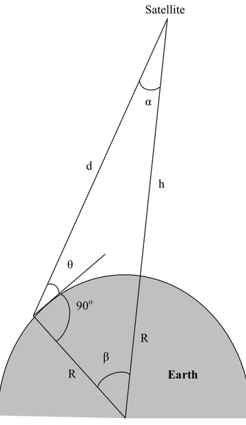
An important factor that determines the coverage area of a satellite is the elevation angle θ of the earth station, which is the angle from the horizontal (that is, a line tangent to the surface of the earth at the antenna’s location) to the point on the center of the main beam of the antenna when the antenna is pointed directly at the satellite. Angle of elevation of 0o yields the maximum coverage of the earth. Figure 1.1 below shows the geometry that dictates the satellite coverage. For downlinks, the elevation angle is about 5o to 20o depending on frequency used as it is in current design practices while uplink is about 5o.

Satellite Earth R R h d

4 The factors that affect the choice of minimum elevation angle include the following;

• Buildings, trees, and other terrestrial objects that would block the line of sight. These may result in attenuation of the signal by absorption or in distortions due to multipath reflection.

• Atmospheric attenuation is greater at low elevation angles because the signal traverses the atmosphere for longer distances when the elevation angle is smaller.

• Electrical noise generated by the earth’s heat near its surface adversely affects reception.

The coverage angle β is a measure of the portion of the earth’s surface visible to the satellite in relation to the minimum elevation angle θ; β defines a circle on the earth’s surface centered on the point directly below the satellite. The equation below describes the relationship between θ and β.

) cos( ) cos( 2 sin 2 sin 2 sin ) sin( θ θ β π θ θ β π π θ α ₌ +       +       _{− −} =       + = +h R R where R = earth’s radius, 6370km

h = orbit height (altitude from point on earth directly below satellite) β = coverage angle

θ = minimum elevation angle

The distance from satellite to farthest point of coverage can be calculated as follows:

) cos( ) sin( 2 sin ) sin( θ β π θ β ₌       + = +h R d

( )

The round-trip transmission delay can be calculated by the formula below:

(

)

where c is the speed of light, approximately 3x108_m/s.

The coverage of a satellite is typically expressed as a diameter of the area covered, which is just 2βR, with β expressed in radians.

Geostationary Earth Orbit (GEO)

This type of communications satellite is very common today probably because of its uses in TV and radio broadcast; they are the type used in weather satellites and satellites operating as backbones for the telephone network. It was first proposed by the science fiction author Arthur C. Clarke in 1945. If the satellite is in a circular orbit 35,863km above the earth’s surface and rotates in the equatorial plane of the earth, it will therefore rotate at exactly the same angular speed as the earth and will remain above the same spot on the equator as the earth rotates. The orbit must have an inclination angle of 0o.

Advantages:

1. GEO satellites do not have problem of Doppler shift because they are stationary relative to the earth.

2. To track the satellite by its earth stations is very simple. Senders and receivers can use fixed antenna positions, no adjusting is needed.

3. It has a very large coverage, at 35,863km above the earth the satellite can communicate with about one fourth of the earth, therefore three geostationary orbit separated at an angle of 120ois enough to cover all the most inhabited portion of the earth.

4. They do not need a handover due to the large foot print. 5. Life expectations for GEOs are very high, at about 15 years.

Disadvantages:

1. The signal gets week after travelling over a long distance of 35,000km.

2. The transmission quality of the signal is further limited by the shading in the cities caused by high buildings and the lower elevation further away from the equator. 3. Northern or southern regions of the earth have more problems receiving these

satellites due to the low elevation above latitude of 60o, therefore large antennas are needed to compensate for this.

4. This type of satellite is not suitable for small mobile devices.

5. The transmitter power required is relatively high which causes problems for battery powered devices.

6. Even at the speed of light, the high latency of about 0.25s one-way is the biggest problem for voice and data transmissions.

7. Frequency reuse is not really possible because of the large footprint. It is a waste of spectrum.

6 HEO GEO (Inmarsat) LEO( Iradium, (Globalstar) MEO (ICO) Km .

Note: The Van Allen radiation belts, are belts consisting of ionized particles, at heights of about 2,000 – 6,000km (inner Van Allen belt) and about 15,000 – 30,000km (outer Van Allen belt) respectively make satellite communication very difficult in these orbits.

Low Earth Orbit (LEO)

LEO satellites revolve on the lower orbit at less than 2000km. Proposed and actual systems are in the range 500 to 1500km; it is obvious that they exhibit a much shorter period typically between 95 to 120 minutes. The diameter of coverage is about 8000km and the round-trip propagation delay is less than 20ms. In addition LEO satellites try to ensure a high elevation for every spot on the earth to provide a high quality communication link. Each LEO satellite will only be visible from the earth for about 10 to 20 minutes. The practical use of the satellite requires the multiple orbital planes be used, each with multiple satellites in orbit. Communication between two earth stations typically will involve handing off the signal from one satellite to another. This technology is being currently used for communicating with mobile terminals and with personal terminals that need stronger signals to function. Inner and outer Van Allen Belts Earth 1,000 10,000 35,863

Advantages:

1. Transmission rates of about 2,400 bit/s can be enough for voice communication if advanced compression schemes are employed.

2. LEO even provides this bandwidth for mobile terminals with omni-directional antennas using a low transmit power in the range of 1W.

3. The small footprints of LEOs allow for better frequency reuse, similar to the concept used in cellular networks.

4. LEO can provide a much higher elevation in Polar Regions therefore there is better global coverage.

5. In addition to the reduced propagation delay mention earlier on, a received LEO signal is much stronger than that of GEO signals for same transmission power.

Disadvantages:

1. To provide a broad coverage over 24 hours, many satellites are needed. Several concepts require 50 – 200 or more satellites in orbit.

2. The short time of visibility with a high elevation demands additional mechanisms for connection handover between different satellites.

3. The short lifetime of about 5 – 8 years due to atmospheric drag and radiation from Van Allen belt is a big problem for LEO satellites.

There is a further classification of LEOs into little LEOs intended to work at communication frequencies below 1 GHz with low bandwidth services (some 100 bit/s), big LEOs work at frequencies above 1 GHz with bandwidth services (some 1,000 bit/s). It uses CDMA as in the CDMA cellular standard. It uses the S-Band (about 2GHz) for the downlink to mobile users, also broadband LEOs with plans reaching into the Mbit/s range.

Medium Earth Orbit (MEO)

Medium Earth orbit satellites can be positioned somewhere in between LEOs and GEOs, both in terms of their orbit, also in their advantages and disadvantages. The circular orbit is at an altitude in the range of 5,000 to 12,000km, the period of the orbit is about 6 hours and the diameter of coverage is from 10,000 to 15,000km while round-trip signal propagation delay is less than 50ms.

Advantages:

1. The system only requires a dozen satellites which is more than a GEO system but much less than a LEO system.

8 4. While propagation delay to earth from such satellites and the power required are

greater than for LEOs, they are still substantially less than for GEO satellites.

Disadvantages:

1. Due to the larger distance to the earth than LEOs delay increases to about 70 – 80ms. 2. The satellites requires higher transmit power and special antennas for smaller

footprints.

Highly Elliptical Orbit (HEO)

These classes of satellites comprises all satellite with non-circular orbit, they are elliptical. Currently few commercial communication systems are planned using satellites with elliptical orbits. These systems have their perigee over large cities to improve communication quality.

1.2.2 Frequency Bands

Table 1.1 below presents the frequency bands available for satellite communications. It is observed that increasing bandwidth is available in the higher-frequency bands. Generally, the higher the frequency, the greater the effect of transmission impairments.

Table 1.1 Frequency Bands for Satellite Communications [1]

Band Frequency Range Total Bandwidth General Application L* 1 to 2 GHz 1 GHz Mobile satellite services (MSS) S* 2 to 4 GHz 2 GHz MSS, NASA, deep space research

C 4 to 8 GHz 4 GHz Fixed satellite service (FSS)

X 8 to 12.5 GHz 4.5 GHz FSS, Military, terrestrial earth exploration and meteorological satellites

Ku 12.5 to 18 GHz 5.5 GHz FSS, broadcast satellite service (BSS)

K 18 to 26.5 GHz 8.5 GHz BSS, FSS

Ka 26.5 to 40 GHz 13.5 GHz FSS

The mobile satellite service (MSS) is allocated frequencies in the L and S-bands. In these bands, compared to higher frequencies, there is a greater degree of refraction and greater penetration of physical obstacles, such as foliage and non-metallic structures. These are desirable characteristics for mobile satellite service. Also the same bands are heavily being used for terrestrial applications. Therefore, there is intense competition among the various microwave services for L and S-band capacity.

For an allocation of frequency to a particular service, there is an allocation of a downlink band and uplink band. The uplink band is usually assigned a higher frequency because higher frequency suffers greater spreading, or free space loss, than its lower frequency counterpart. The earth station is capable of higher power, which helps to compensate for the poor performance at higher frequency.

1.2.3 Benefits of mobile satellite system over terrestrial system.

There are many advantages that mobile satellite communication has over terrestrial wireless communication systems, such merits are enumerated below.

• The area of coverage is a good advantage in satellite base communication which far exceeds that of terrestrial system.

• The speed to deliver new services to the market is a merit of satellite communication over that of terrestrial systems.

• Satellite - to - satellite communication links can be designed with great precision because the conditions between communicating satellites are more time invariant than those between two terrestrial wireless antennas.

• Transmission cost is independent of distance, within the satellite’s area of coverage. In terrestrial wireless system more cost will be incurred to cover as much area as satellite does.

• Broadcast, multicast and point to point applications are already accommodated in satellite communication systems.

• Very high bandwidths or data rates are available to satellite communication users.

• The quality of transmission is normally high in satellite communication than terrestrial although satellite links are subject to short-term outages or degradation.

1.2.4 Thesis structure

Chapter 2 – Propagation channel impairments. In this chapter different types of channel impairments are examined and the basic mechanisms of propagations.

Chapter 3 – Statistical Models. In this chapter, the mathematical representation of the channel is presented for proper descriptions.

Chapter 4 – Implementation of Lutz’s Model. In this chapter the simulation of the Lutz model which describes a channel in two states is implemented.

Chapter 2

Propagation Channel Impairments

In between the transmitter and the receiver is the channel through which the signal travels. In a situation whereby there is no obstacle or obstruction between the transmitter and the receiver there would be a very good quality of transmission but in most cases such an obstacle scenario is impossible.

This chapter presents first the introduction to channel impairments, discuss the basic propagation mechanisms and the different types of impairment that any mobile satellite communication can experience.

12

2.1 Introduction

The mobile radio propagation channel introduces fundamental limitations on the performance of any wireless communication systems. The path of transmission from the transmitter to that of the receiver can vary from just the simple line-of-sight to one that is severely obstructed by mountains, foliage and buildings. With any communication system, the signal that is received will be different from the signal that is transmitted, due to various transmission impairments. For digital data for example bit errors are introduced, a binary 1 is transformed into a binary 0 and vice versa. Same goes for analog transmitted signals, these impairments introduce various random modifications that degrade the quality of the signal. Wired channel are stationary and predictable but radio channels are extremely random in nature and can not be analyse easily. Another factor that affects the channel is the speed of motion which impacts how rapidly the signal level fades as the mobile terminals moves in space. The impairments include attenuation and attenuation distortion, free space loss, noise, atmospheric absorption, multipath, speed of the mobile, the speed of surrounding objects and also the transmission bandwidth of the signal.

2.2 Basic Propagation Mechanisms

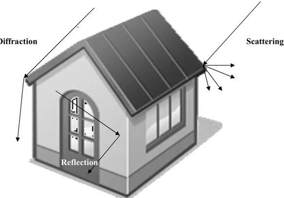
There three basic propagation mechanisms which impact propagation in a mobile communication system namely Reflection, Diffraction and Scatterings [1-3].

Reflection

Reflection happens as a result of a propagating electromagnetic wave impinges upon an object which has very large dimensions when compared to the wavelength of the propagating wave. These reflected waves may interfere either constructively or destructively at the receiver. As an illustration, if a ground-reflected wave near the mobile unit is received, the ground wave and the line-of-sight wave may tend to cancel resulting in high signal loss because the ground-reflected wave has an 180o phase shift after reflection. Also the reflected signal has a longer path which creates a phase shift due to delay relative to the signal not reflected, when the delay is equivalent to half a wavelength then the two signals are back in phase. The reflected signal is not as strong as the original, as objects can absorb some of the signal power. Reflections could occur from the surface of the earth and from the building and walls.

Diffraction

This is a phenomenon where the radio path from the transmitter to the receiver is obstructed by a surface that has sharp edges. When a radio wave encounters such an edge, waves propagate in different directions with the edge as the source. The secondary waves generating from the obstructing surfaces are present throughout the space and even behind the obstacle, giving rise to a bending of waves around the obstacle even when a line-of-sight path does not exist between the transmitter and the receiver. When the frequency is high, diffraction, just like reflection depends on the geometry of the object, the amplitude, phase and the polarization of the incident wave at the point of diffraction.

Scattering

Reflection Diffraction

Figure 2.1 Three Basic Propagation Mechanisms: Reflection, Diffraction and Scattering

14

Scattering

Scattering occurs when the medium through which the wave travels consists of objects with dimensions that are small compared to the wavelength, and where the number of obstacles per unit volume is large. Scattered waves are produced by rough surfaces, small objects, or by other irregularities in the channel. For real the street signs, foliage, and lamp posts induce scattering in a mobile communications system.

2.3 The impairments

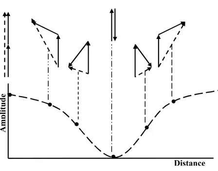
Although the propagation mechanisms discussed above are very important in propagation of radio waves in mobile communication system especially in an environment where LOS is not possible like in an urban setup but at the same time they could pose danger to the performance of a particular channel. As just noted, one unwanted effect of multipath propagation is that multiple copies of a signal may arrive at different phases. If these phases add destructively, as shown in figure 2.2 and 2.3, the signal level declines relative to noise this makes signal detection difficult at the receiver.

First Path (A)

t

Echo Path (B) Case 1

Echo Path (C) Case 2

Constructive Destructive addition addition

(Case 1) (Case 2)

Figure 2.2 Constructive and Destructive addition Of Transmission paths

Transmitted pulse Transmitted pulse Received LOS pulse Received LOS pulse Received mulitipath pulses Received mulitipath pulses Pulse overlap Time Time Distance Amplitude

A second problem which the mechanisms discussed above can cause is intersymbol interference (ISI) which is of great importance to digital transmission.

Figure 2.3 fading as two incoming signals combine with different phases

16 Let us look at a situation whereby a narrow pulse is being sent at a given frequency across a link between a transmitter and a mobile unit, Figure 2.4 above illustrates what the channel may deliver to the receiver if the impulse is sent at two different times. The upper line shows two pulses at the time of transmission and the lower line shows the resulting pulses at the receiver. In each case of the transmissions the first received pulse is the desired LOS signal though reduced in magnitude because of attenuation. In addition to the primary pulse, there may be multiple secondary pulses due to the three basic propagation mechanisms. The overlap of the pulses shows that one or more copies of the pulse arrive at the same time as the primary pulse of the subsequent transmission. These delayed pulses constitute noise in the subsequent primary pulse and therefore making recovery of the information difficult. The other significant impairments are treated below:

Refraction

Refraction occurs because the velocity of an electromagnetic wave is a function of the density of the medium through which it travels. It is only in vacuum that electromagnetic wave such as light or radio wave travels at approximately 3x108 m/s. In other medium like air, water, glass and other transparent or partially transparent media, electromagnetic waves travel at lesser speed than 3x108m/s.

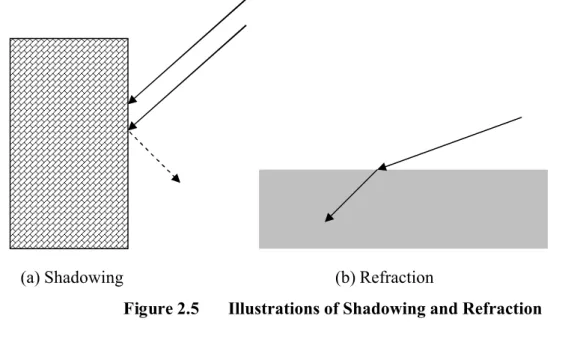
In a situation where an electromagnetic wave moves from a medium of one density to a medium of another density then its speed changes. The effect is to cause a one-time bending of the direction of the wave at the boundary between the two media. Waves that travel into a denser medium are bent towards the medium. This is why LOS radio waves are being bent towards the earth: the density of the atmosphere is higher closer to the ground. Figure 2.5(b) below shows refraction, the shaded portion is the denser region.

(a) Shadowing (b) Refraction

Shadowing

Figure 2.5(a) above describes the blocking or shadowing which is an extreme form of attenuation of radio signals due to large obstacles. The higher the frequency of a signal, the more it behaves like light. Even small obstacles like wall, a truck on the street or trees in an alley may block the signal.

Attenuation and attenuation distortion

Attenuation is a more complex function of distance and the makeup of the atmosphere for an unguided medium. Attenuation introduces three factors for the transmission engineer namely:

• A received signal must have enough strength so that the electronic circuitry in the receiver can detect and interpret the signal.

• To avoid error at the receiver the signal must maintain a level sufficiently higher than the noise.

• At higher frequencies attenuation is greater and it causes distortion.

In other to handle the first two factors amplifier and repeaters are used to maintain good signal strength. The third factor which is attenuation distortion, the received signal is distorted because the attenuation varies as a function of frequency reducing intelligibility. To overcome this problem, techniques are available for equalizing attenuation across a band of frequencies. One approach is to use amplifier that amplifies high frequencies more than lower frequencies.

Free Space Loss

In free space radio signals propagate as light does, they follow a straight path from transmitter to the sender (LOS). The signal still experiences free space loss even if there is vacuum. For any type of wireless communication the signal disperses with distance. For satellite communication this is the primary mode of signal loss. Even if no other sources of attenuation or impairment are assumed, a transmitted signal attenuates over distance because the signal is being spread over a larger area. Free space loss is expressed in terms of the ratio of the radiated power Pt to the power Prreceived by the antenna or in decibels, by taking 10

18 2 2 2 2 _{(4 )} ) 4 ( c fd d P P r t π λ π ₌ = where

Pt= signal power at the transmitting antenna

Pr= signal power at the receiving antenna

λ = carrier wavelength

d = propagation distance between antennas c = speed of light (3x108m/s)

d and λ are in the same unit i.e. meters.

In decibel, we can write

dB d d P P L r t dB 20log( ) 20log( ) 21.98 4 log 20 log 10 _=− + +      = = λ λ π dB d f c fd 56 . 147 ) log( 20 ) log( 20 4 log 20 _= + −      = π

For other antennas we must put into consideration the gain of the antenna, which yields the following free space loss equation:

t r t r t r r t A A f cd A A d G G d P P 2 ) ( ) ( ) ( ) 4 ( 2 2 2 2 2 = = = λ λ π where

Gt= gain of transmitting antenna

Gr= gain of the receiving antenna

At= effective area of the transmitting antenna

Ar= effective area of the receiving antenna

Thus, for the same antenna dimensions and separations, the longer the carrier wavelength (lower the carrier frequency f), the higher is the free space path loss.

Noise

Any unwanted signal that are inserted somewhere between the transmission and the reception is referred to as noise. Noise is the major limiting factor in communications system performance. There are four categories of noise namely Thermal noise, Intermodulation noise, Crosstalk and Impulse noise.

Thermal noise is due to thermal agitation of electrons. It is present in all electronic devices and transmission media and is a function of temperature. It is uniformly distributed across the frequency spectrum hence is often referred to as white noise. This type of noise cannot be eliminated therefore it places an upper bound on communications system performance. It is particularly significant for satellite communication.

The amount of thermal noise to be found in a bandwidth of 1Hz in any device is N0= kT (W/Hz)

where,

N0= noise power density in watts per 1Hz of bandwidth

k = Boltzmann’s constact = 1.3803x10-23 J/K T = temperature, in kelvins (absolute temperature)

Intermodulation noise is as a result of signals at different frequencies share the same transmission medium. This type of noise produces signal at a frequency that is the sum or difference of the two original frequencies or multiples of those frequencies.

Crosstalk is an unwanted coupling between signal paths. It can occur when unwanted signals are picked up by microwave antennas. Typically, crosstalk is of the same order of magnitude as or less than thermal noise.

Impulse noise is noncontinuous, consisting of irregular pulses or noise spikes of short duration and of relatively high amplitude. It is from a variety of causes including external electromagnetic disturbances, such as lightning, faults and flaws in the communications system.

Atmospheric Absorption

Atmospheric absorption is another loss that can be experience between the transmitting antenna and the receiving antennas. Water vapour and oxygen contribute most to this type of loss by attenuating the signal strength.

The Speed of Mobile

The relative motion between the transmitting antenna and the mobile unit results in random frequency modulation due to different Doppler shifts on each of the multipath components. Doppler shift will be positive or negative depending on whether the mobile receiver is

20

Speed of the Surrounding Objects

If objects in radio channel are in motion, they induce a time varying Doppler shift on multipath components. If the surrounding objects move at a greater speed than the mobile, then this effect dominates the small-scale fading. Otherwise this effect could be neglected.

The Transmission Bandwidth of the Signal

If the transmitted radio signal bandwidth is greater than the bandwidth of the multipath channel, the received signal will be distorted, but the received signal strength will not fade much over a local area meaning that the small-scale signal fading will not be significant.

2.4 Types of Fading

The term fading refers to the time variation of a received signal power caused by changes in the transmission medium or paths. In a fixed setup, fading is affected by changes in atmospheric conditions such as rainfall. But it is different in a mobile environment where one of the two antennas is moving relative to the other, the relative location of various obstacles changes over time, creating complex transmission effects. Fading can be classified based on multipath time delay spread and Doppler spread [2].

2.4.1 Fading Based on Multipath Delay Spread

Delay spread is a type of distortion that is caused when an identical signal arrives at different times at the receiver. The signal usually arrives via multiple paths and with different phases. This is the time different between arrival moment of the first multipath component (usually the LOS component) and the last one. There are two types, flat fading and frequency selective fading.

Flat Fading

Flat fading or non-selective fading is a type of fading in which all the frequency components of the received signal fluctuate in the same proportion simultaneously.

• Bandwidth of the signal is smaller than the bandwidth of the channel.

Frequency Selective Fading

Selective fading affects unequally the different spectral components of a radio signal.

• Bandwidth of the signal is larger than the bandwidth of the channel

• The delay spread is greater than the symbol period.

2.4.2 Fading Based on Doppler Spread

This is another type of distortion that is caused when an identical signal arrives at different times at the receiver. As a result of the delay spread, the movement of the mobile unit relative to the transmitter and the movement of surrounding objects, there is shift in the frequency of the signals arriving at different paths. Doppler spread is the different between the highest frequency shift and the lowest frequency shift. There two types of this fading, fast fading and slow fading.

Fast Fading

This is a type of fading occurring with small movements of a mobile or obstacle.

• Higher Doppler spread

• Coherence time less than symbol period

• Channel variations faster than baseband signal variation.

Slow Fading

This kind of fading is caused by larger movements of a mobile or obstructions within the propagation environment.

• Low Doppler spread

• Coherence time is greater than symbol period

Chapter 3

Statistical Models

The design of mobile satellite communication systems to provide the desired communication quality of service (QoS) depends on a good propagation channel model. The satellite channel is dynamic in nature with variety of propagation paths ranging from a clear line-of sight (LOS) path in an open environment to a lightly-shadowed path by foliage where the mobile unit passes through forests, to severe shadowing cases typical of transmission to units located in dense high-rise urban settings. A suitable statistical model should be able to describe the behaviour of a particular channel considering the impairments that can be experienced.

This chapter will present the different types of some of the major statistical models available to describe mobile satellite communication channels.

24

3.1 Introduction

The primary aim of signal modelling of a channel is for the purpose of simulation experiments in other to avoid costly hardware tests of wireless communication systems. Signal modelling plays an important role in this current age in analytical design studies and computer simulation of many systems such as mobile satellite communication and the likes. For a particular model to be really suitable it depends on finding a mathematical description of an experimental data and generating an artificial signal with assumed properties. Such a channel to be described by any model in mobile satellite communication environment is shown below in Figure 3.1. This is a typical scenario where a signal received by the mobile unit comprises of a LOS path and a number of scattered, reflected, diffracted and refracted components. Ionosphere Troposphere Ground Reflection Direct Wave (LOS) shadowing Diffuse component

The first step towards modelling the mobile satellite channel is to identify and categorize typical transmission environment. This is normally done by dividing the environment into three major categories:

• Urban areas which is characterised by almost complete obstruction of the direct

wave (blockage of the Line-of –Sight path).

• Open and rural areas which has no obstruction of the direct wave (there is

line-of-sight path).

• Suburban and tree shadowed environments where intermittent partial obstruction of

the direct wave occurs.

A multipath propagation medium contains several different paths by which signal travels from the transmitter to the receiver. In a case of a stationary receiver we have a static

multipath situation in which a narrowband signal is transmitted and several copies arrive at

different interval at the receiver. But in a situation where either the transmitter or the receiver is in motion, then we have a dynamic multipath situation in which there is a continuous change in the propagation path length therefore the relative phase shifts between the paths change as a function of spatial location [4, 5]. The latter situation is our point of interest in this thesis report.

3.2 The Basic Probability Distribution Functions

Probability distribution functions can be used to describe and characterise the multipath and shadowing phenomena with some degree of accuracy. This type of modeling allows the dynamic nature of the channel to describe therefore the performance of the system can be evaluated for different environments. The essential combinations of three probability function (PDF) are used to model the channel of mobile satellite communication. The PDFs are Rayleigh distribution – when there is no Line-of-Sight (LOS) and multipath reception is dominant, Rician distribution – when Line-of-Sight (LOS) is present and dominant over multipath reception and Log-normal distribution – when no significant multipath reception is present and there is shadowing of the direct wave [6, 11, 13].

3.2.1 Rayleigh Distribution

In an urban environment, the received signal is normally characterised by virtually a complete obstruction of the direct wave. In such a situation the received signal will be

26 uniform probability density function within the range of 0 and 2π, while the amplitude can be categorised by the Rayleigh distribution. This distribution describes the diffuse component and can be expressed as a phasor sum of a number of scattering point sources:

∑

where r is the amplitude of the diffused component, θ is the phase of the diffuse component, φj is the phase of the jth diffuse component with respect the direct component, Aj is the

random amplitude of jth scattered wave with respect to the direct component.

     ₋ = ₂ 2₂ 2 exp ) ( σ σ r r r f_Rayleigh

where r is the signal envelope given by the equation below:

2 2 _y

x

r= +

σ2 is the mean received power of the diffuse components. For unmodulated carrier frequency, fc, the Doppler shift, fd, of a diffuse component arriving at an incident angle θiis

given by: i c d c vf f = cosθ in Hertz.

θi is in the range 0 - 2π. This result in a maximum Doppler shift, fm, of ±vf_c/c, c is the

speed of light 3x108 m/s. Hence at the receiver, a band of signals is received within the range fc±fm, where fm is the rate of fading. For uniform received power for all angles of

arrival at the terminal, the resultant power spectral density is given by this expression:

2 1 2 ) ( 1 2 ) ( −             − − = fm fc f fm f S π σ _(W/Hz)

3.2.2 Rician Distribution

The Rician distribution is used to describe the unshadowed component and it is expressed as a phasor sum of a constant and a number of scattering components:

∑

where C is a constant coherent signal with clear LOS and the rest of the symbols are same as in Rayleigh distribution. In a situation where direct wave is present (Line-of-Sight) as in the case of mobile satellite in an open environment, the representation of the two dimensional probability density function of the received signal is given as below:

, 2 ) ( exp 2 1 ) , ( ₂ 2 2 2    ₋ − + = σ πσ y C x y x P_XY

the probability density function of the random signal envelope is given as:

           ₋ + = 2 0 ₂ 2 2 2 ₂ ) ( exp ) ( σ σ σ rC I C r r r f_Rice

where I0(.) is the modified zero-order Bessel function of the first kind, C2/2 is the mean

received power of the direct wave component, r is the signal envelope and σ2is the mean received scattered power of the diffuse component due to multipath propagation. The above equation reduces to Rayleigh distribution when LOS is absent i.e. C = 0. The power ratio of the direct wave to that of the diffuse component is known as the Rice factor usually expressed in dB, K = A2/2σ2.

3.2.3 Log-normal Distribution

Vegetatively shadowed propagation is described by a lognormal distribution, which arises from a theory of random variables that combines variables by a multiplicative process just as a normal distribution arises from a theory of random variables that combines variables by an additive process. It can be represented mathematically by:

  n n

28 {Bj} is a sequence of independent positive random variables and the phase variables {φj} is

uniformly distributed between 0 and 2π. The effect of shadowing of the direct wave LOS where no multipath is present can be characterised by lognormal distribution and the probability density function is given by:

     ₋ − = 0 2 0 2 ) (ln exp 2 1 ) ( d r d r r f_Lognornal µ π

where r is the signal amplitude, μ is the mean of the shadow component (lnr) and d0= σ is

the standard deviation of the shadowed component (lnr). Random shadowing of the direct wave occurs in the sub-urban environment due to the presence of trees, building and so on.

3.3 The Major Channel models

The difference between major mobile satellite models is the variation in the method of mixing the above three basic distribution functions in right proportions. The models we would examine are named after the investigators who originally proposed them. These are

Loo, Corazza, Lutz, Nakagami and Norton. Alireza Mehrnia and Homayoun Hashemi [6]

have really done a substantial work in investigating and comparing these models, according to their investigation Lutz’ model is the best, followed by Nakagami, Corazza, Loo and Norton in that order. The table 3.1 below is the summary of their report.

Model Open Area Shadowed Area Semi-Open Semi-Shadowed Overall Performance Relative MSE Norton 0.8737 1.3680 1.4593 1.2340 1.8 Loo 0.8107 1.2554 1.4365 1.1680 1.7 Corazza 0.8177 0.9373 0.9316 0.8960 1.3 Nakagami 0.5310 1.0890 0.8622 0.8270 1.2 Lutz 0.4545 0.7823 0.8290 0.6890 1.0

Table 3.1 Least Mean Square Error between Empirical and Theoretical Distributions [6]

3.3.1 Loo’s Model

This model present signal with amplitude that has a Rician distribution with a fixed average power of scattered component, σ2 and a random Line-of-Sight (LOS) described by lognormal distribution. The probability density function (pdf) is shown below:

∫

=

0 ( | ) ( )

)

(r f r C f C dC

f_{Loo Rice Log}

where the parameters are as defined before in the probability distribution functions. The average power of the multipath components is assumed to be fixed, therefore it is constant. It means that the process is stationary that is the surrounding environment does not have impact on the mobile terminal.

Merit: It is suitable to handle situation in an open areas in which the surrounding

environment of the mobile is uniform and the LOS component is much stronger than the multipath components.

Demerit: This model is not being suitable to describe the channel in dense urban area where

random numerous multipaths are present since it does not predict fast fading.

3.3.2 Corazza’s Model

The effect of the lognormal (shadowed) component (S) appears in a multiplicative form on the Rice component (R) in this model, that is r = RS (R is Rician distributed and S is lognormal distributed). Due to the independence between R and S we have below the probability distribution function of Corazza’s model with amplitude r.

∫

f_{Corazza Rice Log}

The Rice probability distribution function is conditioned on the shadowing from the above equation.

30

Merit: The effect of slow fading (shadowing) has been included in both the LOS and the

multipath components.

Demerit: It may not be a proper model to describe a dense urban setting unless the

parameters are well chosen to handle such. The shadowing affects both the LOS and multipath components. As a result the LOS and the multipath (Rayleigh) components are influenced by the fading factor. For clear LOS topography Corazza’s distribution does not provide a performance as good as Rice.

3.3.3 Lutz’s Model

The Lutz’s model incorporates Suzuki model (which mixes Rayleigh distribution and lognormal distribution together in good proportion) with the Rice distribution function to describe a perfect scenario of a mobile satellite communication. It describes two states “good” and “bad” channel. The Suzuki model describes the bad channel in which intervening obstacles block the LOS path and information is received through the NLOS path while the Rician distribution describes the good channel which is characterised by a clear LOS component and the received signal is strong. This is a total shadowing model. Below shows the probability distribution functions of Suzuki and Lutz model.

∫

= _{0 ( |} 2_{) (} 2₎ 2

)

(r f r σ f σ dσ

f_{Suzuki Rayleigh Log}

where A and (1-A) are percentages of shadowing and unshadowing respectively, all other parameters remain the same as used before.

Merit: It is suitable to describe all mobile environments. Demerit: It has a lot of parameters.

3.3.4 Nakagami’s Model

This distribution is also known as the m-distribution, it is a general formula for fading, and it contains many other distributions as special cases. It allows the length of the scatter vectors to be random which may not be possible in Rayleigh distribution. The probability density function is stated below with r being the amplitude:

2 1 , exp ) ( 2 2 ) ( 2 1 ≥       Ω − Ω Γ = − mr m m r m r f _m m m Nakagami

where Г(m) is the Gamma function, Ω = E{r2}and m = {E[r2]}2/Var[r2], with the constraint m ≥ ½.

Merit: This distribution reduces to Rayleigh for the value of m = 1 and to one-sided

Gaussian distribution for m = ½. It also approximates the Rician distribution with high degree of accuracy and under certain condition approaches the lognormal distributions.

Demerit: It does perform well in describing a typical channel because of the great variations

in the type of environment, for the Semi-LOS and Semi shadowed paths.

3.3.5 Norton’s Model

The distribution has originally been proposed for point to point microwave link, it is similar to the Nakagami’s model. Somehow it combines both Nakagami and Rice distributions together as given by its probability density function. r is the amplitude of the signal.

                + − = − 2 −1 2 2 2 1 2 exp ₂ ) ( σ σ σ ram I m a r a m r r fNorton _{m m} m where a ≥ 0, and m = ≥ ½.

Demerit: The performance is for mobile satellite communication probably because it was

Chapter 4

Implementation of Lutz’s Model

This is the total shadowing model as it is called which classifies the propagation channel as “good” and “bad”. The good channel is described by a Rician distribution where there is clear LOS and a strong received signal while the bad channel is described by another model called Suzuki which is the combination of Rayleigh distribution in which multipath component of the waves is characterized and Lognormal distribution in which the shadowed component of the direct wave is characterized. The probability density function of Lutz’s model is shown in chapter 3 above.

In this chapter how Lutz’s model is implemented is presented and we would use the cumulative fade distribution to see if a channel is good or bad.

34

4.1 Introduction

Several models have been authored in the past years to describe the propagation channel of mobile satellite communication systems and Lutz’s model happen to be one of the most popular out of the major models. The popularity may be as a result of its description of two state channels and probably because it is a mixture of another model (Suzuki) with the Rician distributions.

The data set generation of Rayleigh distribution, Rice (unshadowed) distribution, lognormal distribution, Suzuki model distribution otherwise known as shadowed distribution (addition of Rayleigh and lognormal distributions), the total (shadowed + unshadowed) data set generation for simulation of Lutz’s model is discussed for the purpose of the implementation.

4.2 Generation of Statistical Distributions

4.2.1 Generation of Rayleigh/Rician data set

A Rayleigh or Rician distribution data set can be generated by using the sum of random phasors as stated in Chapter 3 above.

If the complex-value data is decomposed into a real and imaginary part, both having normal distribution with zero mean and one variance, we then have [11];

∑

∑

∑

∑

all symbols are same as used before, in the case of Rician data set generation, C which is the direct component of the wave (LOS) and it is assumed to be one is added to the above equations.

The Rayleigh distribution is defined by its carrier-to-multipath power ratio K in dB and K is used to define the carrier-to-multipath power ratio of Rician distribution in dB. The relationship between the K and Rayleigh mean square value α (mean square value of

_2σ2 _{=α =10}−K10 _{and scaling factor =}

n α

The PDF of Rayleigh distribution using parameter α becomes,

        − = − − ₁₀ 2 10 ₁₀ exp 10 2 ) ( K K Rayleigh r r r f

,

while the relationship between the K and Rician mean square value β (mean square value of scattered component r and C which is the amplitude of the direct wave) is;

10 10

2 _{10 10}

2σ =β =C⋅ −K = −K , C = 1 and the scaling factor =

n β

The PDF of Rice distribution using parameter β becomes,

       _{− +} = − − 10 0 2 10_{( 1) 2} 10 exp 2 ) ( K K Rice r r r I r f

For the simulation the use of Random Number Generator (RNG), randn(n,m), in Matlab is employed, where the parameter n represents the number of scattered phasors and m represents the number of points which could be in time or distance. n is chosen not to be lower than 5 based on central limit theorem while we need at least about 10000 samples (m) for statistical accuracy of 0.1 percent.

4.2.2 Generation of Lognormal data set

A multiplicative process of random variables is used in the generation of lognormal data set rather than the sum of random phasors.

      = =

∏

∑

36 The derived equation for lognormal data set is seen below;

(

)

∑

The lognormal PDF is specified by μdBand σdB; µ µ_dB =(20loge) σ σ_dB =(20loge) r e r (20log )ln log =      ₋ − = ₂ 2 2 ) log 20 ( exp 2 log 20 ) ( dB dB dB Lognornal r r e r f σ µ π σ

4.2.3 Generation of Shadowed data set

The shadowed data set is the phasor sum of Rayleigh data set and lognormal data set as shown before in earlier discussion.

ϕ φ θ j j j Rayleigh Lognormal Shadowed R R r e z e w e R = + = ⋅ = ⋅ + ⋅

The phases φ, are uniformly distributed, z has lognormal distribution and w has Rayleigh ϕ distribution.

4.2.4 Generation of Unshadowed data set

The Rician distribution discussed above is the unshadowed distribution used to generate the data set.

∑

4.2.5 Generation of Total data set

To generate the total data set, the shadowed and unshadowed (Rician) data set are combined according to the percentage of shadowing S. The total signal is a simple concatenation of shadowed and unshadowed data set with respect to the percentage of shadowing.

Unshadowed Shadowed

Total S R S R

R = ∗ +(1− )∗

4.2.6 Propagation Model Parameter for Typical LMSS

Values within the range of the table below is used for the simulation, we are considering a narrowband signal in this report operating at the frequency band of 2 – 4 GHz.

10 dB < K < 22 dB

10 dB < K < 18 dB

-1 dB < µ < -10 dB 0.5 dB < _{σ < 3.5 dB}

Chapter 5

Results and Conclusion

There are five parameters that determine how the result of the simulation will look like, the shadowing time-share, S which is in percentage, the Rician factor, K in dB, the Rayleigh factor, K in dB, the mean of the lognormal distribution, μ in dB and the standard deviation

of the lognormal distribution, σ in dB. Table 4.1 presents the ranges of values that are suitable as confirmed from different measurements. The appropriate values of the parameters were chosen and the result of simulation shows good agreement with the analytical result when compared.

This last chapter present the graphical results of the simulation which comprise the generation of Lognormal, Rayleigh, Rician and Shadowed distribution data set and their probability density functions as compared with the analytical probability density functions. Also the generation of total distribution data set and its cumulative fade distribution as compared with the analytical CFD is presented in this chapter.

The performance characteristic of the channel in the form of the Bits Error Rate is also discussed here.

40

5.1 Simulation Results

The results of the simulation are presented in this section as shown below in the figures. The changing factor in the simulation is the time-share of the shadowing while other factors are kept constant because the time-share of the shadowing is the predominant factor that affects the channel propagation as revealed from the results. Therefore 25% and 70% of the time-share of shadowing were used to generate the data set and compare with the analytical model results of the various distributions presented in this thesis.

Figure 5.1 to 5.5 are the results of 25% time-share of the shadowing, for the simulation the following parameters were used; S = 0.25, K = 6 dB, K = 5 dB, μ = -3 dB, σ = 5 dB. In

figure 1-4, lognormal, Rayleigh, Rician (unshadowed) and the shadowed (combination of lognormal and Rayleigh) distribution data set were generated and compared with the analytical results, it is seen from the results that the signal envelopes show a good agreement. Figure 5, present the Cumulative Fade Distribution of the generation of the total (shadowed and unshadowed) data sets. It is more convenient to work with fade exceedance distributions. Fade level is defined as the negative of signal level. The CFD is used primarily to evaluate the satellite propagation link. The graph shows a perfect agreement between the simulated and the analytical results.

Figure 5.6 to 5.10 are the results of 70% time-share of the shadowing, for the simulation the following parameters were used; S = 0.7, K = 6 dB, K = 5 dB, μ = -3 dB, σ = 5 dB. The

simulation results of the distributions show agreement with the analytical results also, though there was an insignificant difference in the CFD of the total data set.

It is observed from the results from the CFD of both 25% and 70% time-share of shadowing that for us to achieve the same result in 70% as in 25% time-share of shadowing; we would require more signal energy for the same operation.

0 50 100 150 -40

-20 0

Lognormal data set

Position, meter Signal Level(R),dB 0 0.5 1 1.5 2 2.5 3 3.5 4 4.5 5 0 0.5 1 1.5 Lognormal PDF Signal Amplitude(r) PDF(p(r)) Simulation Analytical

Figure 5.1 Generation of Lognormal data set and the PDF (25% Shadowing)

0 50 100 150

-40 -20 0

Rayleigh data set

Position, meter Signal Level(R),dB 0 0.5 1 1.5 2 2.5 3 3.5 4 4.5 5 0 0.5 1 1.5 2 Rayleigh PDF Signal Amplitude(r) PDF(p(r)) Simulation Analytical

42

0 50 100 150

-40 -20 0

Unshadowed(Rician) data set

Position, meter Signal Level(R),dB 0 0.5 1 1.5 2 2.5 3 3.5 4 4.5 5 0 0.5 1 1.5 Unshadowed(Rician) PDF Signal Amplitude(r) PDF(p(r)) Simulation Analytical

Figure 5.3 Generation of Unshadowed (Rician) data set and the PDF (25% Shadowing)

0 50 100 150

-40 -20 0

Shadowed data set

Position, meter Signal Level(R),dB 0 1 2 3 4 5 6 0 0.5 1 Shadowed PDF Signal Amplitude(r) PDF(p(r)) Simulation Analytical

0 50 100 150 -40

-20 0

Total signal data set

Position, meter Signal Level(R),dB -5 0 5 10 15 20 100 101 102

Cummulative Fade Distribution

Fade level(F),dB

%Time fade > abscissa

Simulation Analytical

Figure 5.5 Generation of Total data set and the CFD (25% Shadowing) The parameters used for the above figures 5.1 – 5.5 are S = 0.25, K = 6 dB, K = 5 dB, μ = -3 dB, σ = 5 dB.

44

0 50 100 150

-40 -20 0

Lognormal data set

Position, meter Signal Level(R),dB 0 0.5 1 1.5 2 2.5 3 3.5 4 4.5 5 0 0.5 1 1.5 Lognormal PDF Signal Amplitude(r) PDF(p(r)) Simulation Analytical

Figure 5.6 Generation of Lognormal data set and the PDF (70% Shadowing)

0 50 100 150

-40 -20 0

Rayleigh data set

Position, meter Signal Level(R),dB 0 0.5 1 1.5 2 2.5 3 3.5 4 4.5 5 0 0.5 1 1.5 2 Rayleigh PDF Signal Amplitude(r) PDF(p(r)) Simulation Analytical

0 50 100 150 -40

-20 0

Unshadowed(Rician) data set

Position, meter Signal Level(R),dB 0 0.5 1 1.5 2 2.5 3 3.5 4 4.5 5 0 0.5 1 1.5 Unshadowed(Rician) PDF Signal Amplitude(r) PDF(p(r)) Simulation Analytical

Figure 5.8 Generation of Unshadowed (Rician) data set and the PDF (70% Shadowing)

0 50 100 150

-40 -20 0

Shadowed data set

Position, meter Signal Level(R),dB 0 0.5 1 Shadowed PDF PDF(p(r)) Simulation Analytical

46

0 50 100 150

-40 -20 0

Total signal data set

Position, meter Signal Level(R),dB -5 0 5 10 15 20 100 101 102

Cummulative Fade Distribution

Fade level(F),dB

%Time fade > abscissa

Simulation Analytical

Figure 5.10 Generation of Total data set and the CFD (70% Shadowing) The parameters used for the above figures 5.1 – 5.5 are S = 0.7, K = 6 dB, K = 5 dB, μ = -3 dB, σ = 5 dB.