Credits: 16 hp Level: G2
Supervisor: Milagros Izquierdo,
Department of Mathematics, Linköping University Examiner: Göran Bergqvist,
Department of Mathematics, Linköping University Linköping: December 2017
topology and naturally this is where the work begins. Topological concepts such as topological spaces, homeomorphisms, and homology are considered. There-after knot theory, and in particular, knot theoretical invariants are examined, aiming to provide insights into why it is difficult to answer the question "How can we tell knots appart?". In knot theory invariants such as the bracket poly-nomial, the Jones polynomial and tricolorability are considered as well as other helpful results like Seifert surfaces. Lastly knot theory is applied to DNA, where it will shed light on how certain enzymes interact with the genome.
Keywords:
Knot theory, Topology, Homology, Jones polynomial, Bracket polynomial, Tangles, DNA.
URL for electronic version:
http://urn.kb.se/resolve?urn=urn:nbn:se:liu:diva-144294
believed in me even when I did not believe in myself.
To my supervisor Milagros Izquierdo I would like to say thank you for your patience, support, feedback and guidance, and to my examiner Göran Bergqvist I wish to express my gratitude for your thorough review which has ensured the quality of this work. I am also thankful for all the valuable thoughts and feedback given to me by my opponent Erik Bråmå on how to improve my work. Last but "knot" least I wish to thank my boyfriend Kalle Trenter for his understanding and unending support, as well as all of my friends and colleagues for hours of interesting discussions.
A The closure of a set A. A⇥ B The Cartesian product. G' H Two isomorphic groups. e0 The Trivial group {0}.
Z The integers (infinite cyclic group). Zn The cyclic group of order n.
X, Y Topological spaces.
Xn, XN Finite and infinite product spaces.
hKi Kauffman polynomial of a link K. (a, b) The open interval {x 2 R : a < x < b}. [a, b] The closed interval {x 2 R : a x b}. ¯
T The usual topology on R. ˆ
T The half-open topology on R.
A\ B The (relative) complement {x 2 A :/2 B}.
f 1(A) The preimage of a set A, i.e. {x 2 X : f(x) 2 A}.
X ⇠= Y Two homeomorphic spaces. Int(A) The interior of a set A. [z], ¯z The equivalence class of z. Cn(K) The group of n-chains.
Zn(K) The group of n-cycles.
Bn(K) The group of n-boundaries.
Hn(K) The n:th homology group.
K A complex in homology and a knot in knot theory. ⌦ Equivalence of knot diagrams.
2 Background 3 2.1 Algebra . . . 3 2.2 Topology . . . 6 2.2.1 Topological Spaces . . . 7 2.2.2 Homeomorphisms . . . 15 3 Homology 21 3.1 Complexes . . . 21
3.2 The Algebra of Chains . . . 24
3.3 Homology Groups . . . 28
4 Knot Theory 35 4.1 Introduction to Knot Theory . . . 35
4.2 Prime Decomposition Theorem . . . 41
4.3 Bracket Polynomial . . . 43
4.4 Jones Polynomial . . . 46
5 Tangles and DNA 49 5.1 Tangles . . . 49
5.2 DNA . . . 53
5.3 Summary . . . 55
2.2 Four examples of topologies from Example 2.2.6. . . 9
2.3 Unit disk to hemisphere. . . 11
2.4 Torus: S1 ⇥ S1. . . 13
2.5 Möbius strip. . . 16
2.6 Cantor set binary tree - by Sam Derbyshire [16]. . . 17
3.1 Examples of simplexes. . . 22
3.2 Four surfaces: sphere, torus, Klein bottle, and projective plane. . 23
3.3 Orientations of 2-cells. . . 24
3.4 A complex on K2. . . 26
3.5 Boundaries of cells. . . 27
3.6 Complex K for Example 3.3.8. . . 32
4.1 Figure 8 knot. . . 36
4.2 Knot table - by Wikipedia user Jkasd [22], published with per-mission. . . 36
4.3 Wild knot - by Wikipedia user Jkasd [21], published with permis-sion. . . 37
4.4 Unknot in disguise. . . 39
4.5 Tricoloring of trefoil. . . 39
4.6 Positive and negative crossing. . . 40
4.7 Seifert surface for 51. . . 42
4.8 Bracket polynomial for the Hopf link. . . 44
4.9 Crossings for the skein relation . . . 47
5.1 Two examples of tangles. . . 50
5.2 Numerator and denominator of a tangle. . . 50
5.3 Tangle sum . . . 51
5.4 Exceptional tangles . . . 51 5.5 Orientations of vertical and horizontal twists . . . 52
Knot theory is the mathematical theory of knots. At this stage, you can think of a knot as a piece of string that you have tied and then glued the ends together. At first glance it might seem like a very unusual mathematical field. Does it really have any practical use? - Yes, it most certainly does! Knot theory can be applied to several areas, one of them being in the study of DNA.
DNA is the genetic code of every living thing and biologists study it with the purpose of better understanding life. Deeper knowledge about DNA would not only give more information about evolution, but it would also make it possible to find new and improved disease treatments. Because DNA is the instruction to how we function it is involved in several processes, processes that aim to decode or extract the information, or to improve or change the information. There are also processes that focus on keeping the DNA "tidy" to ensure that other processes work smoothly. The processes are conducted by enzymes. Enzymes facilitate reactions; some break down the food we eat, some help decode the genome and some are used in industry applications such as producing medicine. One group of enzymes called recombinase manipulate the genome by genetic recombinations. Recombinase can move one segment of DNA to another location on the genome or it can insert alien DNA into the genome. The latter is a key part of the life cycles of some viruses. Understanding the actions of some of these enzymes can be achieved by combining biology with mathematics. Tangle theory (a part of knot theory) can be used to understand how recombinase enzymes interact with DNA. [1]
To utilize the theory of tangles, one must first build a good basis in knot theory, looking for answers to questions like "What is a knot (mathematically)?" and "How do we tell knots apart?". The first question may seem trivial but it took some time before the definition of a knot was put on a firm mathematical
base. The second question is in fact one of the biggest unsolved questions in the field. Today, many knots can be distinguished from one another but there is still no invariant that can fully classify all knots. An invariant is a property of an object that never changes. Invariants help us tell objects apart. The invariant cannot change with the representation of the object but needs to remain the same. There are many thing that can be an invariant, e.g. a number, a polynomial, a group. Studying invariants will be a red thread throughout this work, not only invariants for knots but also for more general objects such as spaces.
The theory of knots is a subfield to the field known as topology. Topology can be described as the study of which properties of objects are left unchanged under continuous deformations. Topologists study ways to tell objects (often spaces) apart, and knot theory utilizes many of the tools and techniques found in topology.
This bachelor thesis will begin with a mathematical background, Chapter 2, that includes concepts from both algebra and topology. In the section on topology homeomorphisms, a concept central to this work, is described. In Chapter 3 the theory of homology is developed. Homology is a powerful tool used to study the structure of spaces. After Chapter 3 we have gained enough topological understanding to dive into Chapter 4: the theory of knots. This chapter covers many concepts in knot theory, however, it is still just a taste of all the wonders this field has to offer. This chapter is concluded by the Jones polynomial, a strong invariant for knots. In the final chapter, Chapter 5, tangles are described as well as some fantastic results they have given to the field of DNA-research.
This chapter covers preliminary concepts needed for the rest of this thesis. Both algebraic concepts (such as groups and rings) and topological concepts (such as topological spaces, continuity and compactness) are described. A big part of the section on topology are homeomorphisms, as they are essential to the rest of this thesis.
2.1 Algebra
In this section we shall go through some important concepts in algebra. A good account of algebraic concepts can be found in [18] and [11]. The key concept in this section will be Polynomial rings.
Definition 2.1.1. A Group, denoted (G, ⇤), is a set of elements G together with an operation ⇤, that satisfy the following properties
1. Associativity: ⇤ is associative, i.e. (x ⇤ y) ⇤ z = x ⇤ (y ⇤ z) for all elements x, y, z2 G.
2. Identity element: There exists a unique identity element, e 2 G s.t. e⇤x = x⇤ e = x for all x 2 G.
3. Inverse: For each element x 2 G exists an inverse x 1 s.t. x ⇤ x 1 =
x 1
⇤ x = e.
Moreover, if the operation is commutative (x ⇤ y = y ⇤ x) then the group (G, ⇤) is called an abelian group.
Example 2.1.2. The set Z of integers together with addition form a group, (Z, +). Addition with integers is associative, it has the identity element 0, and
8x 2 Z, 9y 2 Z : x + y = 0, y is the inverse and can also be denoted x. (Z, +) is abelian. N with addition is an simple example of a set that fails to be a group. Definition 2.1.3. A group G is called cyclic if it can be generated by a single element a, such that G = hai = {k ⇤ a : k 2 Z}.
Example 2.1.4. Z is a cyclic group Z = h1i = {1 ⇤ k : k 2 Z}.
The order of a finite group is the number of elements in the group. The set of (positive) integers modulo n form the finite cyclic group Zn of order n.
The rank, rk(G), of a group G is the minimum number of generators needed to generate G. For example Z ⇥ Z ⇥ Z = Z3has rank 3, and every cyclic group
(e.g. Z6) has rank 1.
Definition 2.1.5. Let (G, ⇤G), (H, ⇤H)be groups. A homomorphism h : G !
H is a function such that 8g1, g22 G it holds that h(g1⇤Gg2) = h(g1)⇤Hh(g2).
An isomorphism is when we also require h to be a bijection. Two groups are therefore called isomorphic, denoted G ' H if there is exists an isomorphism between them.
Example 2.1.6. The most general abelian group is a product of cyclic groups, finite or infinite, and can therefore be written as
Zr
⇥ Zn1⇥ ... ⇥ Znk
where r is the rank. This a actually a very powerful result called the Structure Theorem and a proof can be found in [18].
From groups we now go on to create something called rings.
Definition 2.1.7. A Ring, denoted (R, +, ⇤), is a set of elements R together with two operations + and ⇤, called addition and multiplication respectively, that satisfy the following properties
1. (R, +) is an abelian group. 2. ⇤ is associative.
3. ⇤ is distributive over +, meaning that x ⇤ (by + z) = (x ⇤ y) + (x ⇤ z) and (x + y)⇤ z = (x ⇤ z) + (y ⇤ z) hold for all x, y, z 2 R.
If ⇤ is commutative we way that R is a commutative ring.
Example 2.1.8. Several of the most common sets of numbers Z, Q, R, C together with normal addition and multiplication are rings. As is Mn(R), the
Definition 2.1.9. Let R be a ring, then a polynomial p in x over R is a formal sum p(x) = 1 X k=0 akxk
where ak 2 R for all k and all but a finite number of ak = 0. The set of all such
polynomials is denoted R[x].
The set of polynomials R[x] is a ring with addition and multiplications de-fined as follows.
Definition 2.1.10. 1. The sum of two polynomials, p1(x) = P1k=0akxk
and p2(x) =P1k=0bkxk where ak, bk2 R, is defined as
p1(x) + p2(x) = 1
X
k=0
(ak+ bk)xk.
2. The product of two polynomials p1(x)and p2(x) is defined as
p1(x)p2(x) = 1 X k=0 ckxk, where ck=Pkj=0ajbk j.
Looking at the definitions we see that addition and multiplication are done in the same fashion that we are used to. We add term by term and we multiply "crosswise".
Example 2.1.11. If Z6is the set of integers modulo 6, with normal addition and
multiplication, modulo 6, the (Z6, +,⇤) forms a ring. Now, let p1(x) = x2+x+3
and p2(x) = 2x + 4be two polynomials in the ring Z6[x], then
p1(x) + p2(x) = (x2+ x + 3) + (2x + 4) =
= x2+ (1 + 2)x + (3 + 4) = = x2+ 3x + 1
and
p1(x)p2(x) = (x2+ x + 3)(2x + 4) =
= (1⇤ 2)x3+ (1⇤ 4 + 1 ⇤ 2)x2+ (1⇤ 4 + 3 ⇤ 2)x + (3 ⇤ 4) = = 2x3+ 4x.
Definition 2.1.12. A field F is a commutative ring R with identity 1, in which every nonzero element has a multiplicative inverse.
This means that if R is a field (R, ⇤) is an abelian group.
Definition 2.1.13. A Laurent polynomial with coefficients ai in a field F , is
the formal sum
p(x) =X
k
akxk, k2 Z,
with finitely many of the coefficients nonzero.
Simply put, a Laurent polynomial is a polynomial for which we allow neg-ative powers of x. We denote the collection of polynomials over the field F by F [x, x 1]. F [x, x 1]is a ring.
2.2 Topology
There are many concepts in knot theory that most people intuitively can un-derstand. This allows for interesting and easy introductions in popular science (but oddly enough, most people are still unaware of knot theory). However, in order to dive deeper into knot theory, to be able to fully understand it, we first need to learn some topology. This section is meant to give readers who have not taken a course in topology enough background to be able to follow and understand the concepts of this thesis. We follow the books [2], [5], and [11] in this section.
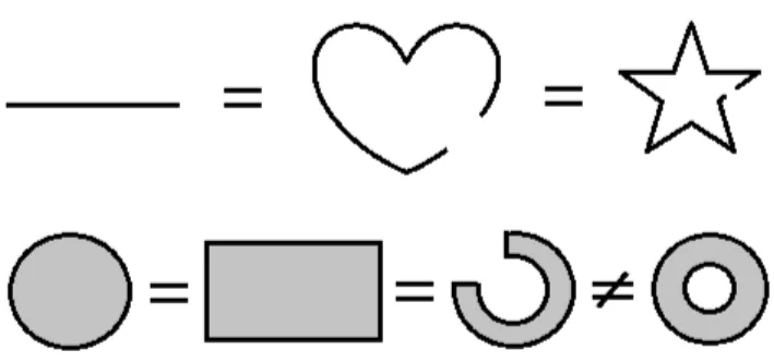
In topology we rid ourselves of the concepts of distance when determining if two objects are near. Transforming spaces continuously is a cornerstone in this thesis. If you, by using for example stretching and bending, can transform A into B, and B into A, you can consider them to be the same, this is the notion of homeomorphisms. Homeomorphisms give equivalence between spaces and we wish to study properties that remain intact under homeomorphisms. We must be very restrictive with operations such as cutting and pasting. Combinations of these are often not continuous and can therefore yield non-homeomorphic spaces. See Figure 2.1. To emphasize the concept of homeomorphism we begin will the following definition.
Figure 2.1: Examples of homeomorphisms.
Definition 2.2.1. Let A and B be topological spaces. Then A is topologically equivalent or homeomorphic to B if there is a continuous invertible function f : A! B with continuous inverse f 1: B
! A. Such a function f is called a homeomorphism.
We need more knowledge to fully grasp this definition. In the following sections all needed concepts will be explained.
2.2.1 Topological Spaces
A topological space is a very general concept of a space. Later we will see that metric spaces are specializations of topological spaces where the topology is given by distances.
Basic concepts
Definition 2.2.2. A topological space is a set X with a collection B of collections Bx, for all x 2 X, of nonempty subsets N ✓ X, called neighborhoods, such that
• every point is in some neighborhood, i.e.,
8x 2 X, 9N 2 Bxsuch that x 2 N
• the intersection of any two neighborhoods of a point contains a neighbor-hood of the point, i.e.,
• for every neighborhood N of a point there is a smaller neighborhood N0
such that each point in N0 has a neighborhood contained in N, i.e.,
for N 2 Bx, 9N02 Bx such that 8y 2 N0 there is some Vy2 By with Vy⇢ N.
The set Bx is called a neighborhood basis for x, and B = [Bx generate a
topology as follows: a subset O ✓ X is an open set if for each x 2 O, there is a neighborhood N 2 B such that x 2 N and N ✓ O. The set T of all open sets is a topology on the set X, and the set B is called a basis for the topology on X. Remark. By this definition ; is always open.
For a set X with topology T we will use the notation (X, T) to refer to the topological space. However, when there is no ambiguity, this notation will sometimes be abused and X will stand for a topological space.
In the beginning of this section we mentioned that a metric space is a topo-logical space, we shall now look at the Euclidean space.
Example 2.2.3. With the Euclidean distance metric in Rn,
d(x, y) =p(x1 y1)2+ (x2 y2)2+ ... + (xn yn)2,
we can form n-dimensional balls, B(x, r) = {y 2 Rn : d(x, y) < r
} of radius r > 0, around any point x. Together these balls form a basis B = {B(x, r) : x2 Rn, r > 0
} for the topology on Rn.
More generally: If X is a set with a metric d (metric space), then the set of balls B = {B(x, r), x 2 X, r > 0} is a basis for a topology on X, where B(x, r) ={y 2 X : d(x, y) < r} for r > 0.
Example 2.2.4. For R we construct B = {(a, b) : x 2 R, a < x < b}, the set of all open intervals on R. The topology ¯T given by B is called usual topology on R. The open neighborhoods are (a, b).
The construction of topology above is equivalent to the topology in Theorem 2.2.5 that is stated below. This theorem can be taken as the definition of a topology.
Theorem 2.2.5 (cf. [11]). T is a topology on X iff 1. X and ; are elements of T.
2. The union of any collection of elements in T is in T.
3. The intersection of any finite collection of elements in T is in T. Theorem 2.2.5 gives a new way to determine if T is a topology on a set X.
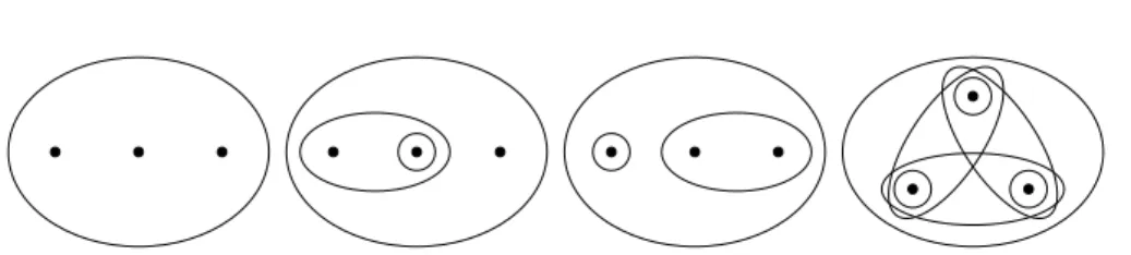
Figure 2.2: Four examples of topologies from Example 2.2.6.
Example 2.2.6. Let X = {x, y, z} be three points. Four examples of topologies on X can be found in Figure 2.2. They are (from left to right):
• T1={;, X},
• T2={;, {y}, {x, y}, X},
• T3={;, {x}, {y, z}, X}, and
• T4={;, {x}, {y}, {z}, {x, y}, {x, z}, {y, z}, X}.
Non of these topologies are homeomorphic to one another. The first one {;, X} is called the trivial topology, and the last one is called the discrete topology on X. There are several more topologies on X - simply find other combinations of subsets that satisfy Theorem 2.2.5.
Definition 2.2.7. Let C be a subset of a topological space X with topology T, then we say that C is closed if X \ C is open.
Example 2.2.8. Let X = {x, y, z}, T = {;, {y}, {x, y}, {y, z}, X}, C1 = {x}
and C2={x, y}. Are C1and C2closed? Well, C1is closed if the complement is
open (i.e. X \ C1✓ T). X \ C1={y, z} ✓ T so X \ C1is open and C1is closed.
Similarly, X \ C2={z} 6✓ T so X \ C2 is not open and therefore C2 cannot be
closed.
Open and closed sets depend on our choice of basis and topology. Changing them may change which sets we consider to be open and closed - altering all concepts that in turn depend on these, such as, compactness and continuity.
This makes things a little abstract. For instance, the trivial topology has only one neighborhood N = X. ; and X are, by definition, the only open and the only closed sets.
From the definition of neighborhoods we get that they can be any non-empty set, so one neighborhood of the point x could be {x}. For the discrete topology we have that any subset of X is both open and closed.
For R the standard neighborhoods are the open intervals (a, b) and the usual topology is the set of all of these open intervals, as seen in Example 2.2.4. On R there is a different, very interesting, topology called the half-open topology.
Example 2.2.9. Let the interval [a,b) with a, b 2 R, be a neighborhood 8x 2 [a, b). There is a topology ˆT on R where set of intervals B = {[a, b)} form a basis for ˆT. ˆT is called the half-open topology. The interval [1, 2) will be a neighborhood for the point 1, and is by definition an open set. Furthermore this half-open topology is fundamentally different form the usual topology with open neighborhoods (a, b), because there is no interval of the form (a, b) that is a neighborhood of 1 and also a subset of [1, 2).
The following definition gives us a property that makes spaces nice and informative to study.
Definition 2.2.10. A topological space is Hausdorff if, for any two distinct points in X, there are disjoint open sets, one containing one of the points, the other containing the other.
That a space is Hausdorff is a good property to have. It means that we can study each point individually, it is not hidden in a cluster of points. All spaces we will be working with are Hausdorff. In numerical analysis if you consider a situation where you have data from real numbers and an error margin, the resulting space will not be Hausdorff. Computers only allow a finite (in many cases fixed) number of decimals, and hence does not save enough information to study every point in R individually. There are several intervals in which you cannot tell points apart. This problem is common in real applications on data sets.
Example 2.2.11. Both (R, ¯T) and (R, ˆT) are Hausdorff.
Example 2.2.12. In Example 2.2.6 only T4 is Hausdorff. In T3, for example,
we can never study just the point z, we must always consider y and z together. From a topological space (X, T) we can create a new space by taking a subset Aof X and using T to induce a topology on A. The following definition explains how.
Definition 2.2.13. Let X be a topological space with topology T and let A ✓ X. A neighborhood of a point x 2 A relative to A is of the form N \A where N is a neighborhood of x in X. The topology TAgenerated by this basis is called
the subspace topology on A induced by the topology T on X.
From any topological space we can make new subspaces by using this method-ology. The neighborhoods in the subspace topology (N \ A) are open relative to A, but not necessarily open relative to X. For the Euclidean space with the normal topology (see Example 2.2.3) we can take any subset and induce a sub-space topology. For some subsets (e.g. closed ones) there will be neighborhoods in the subspace topology that are not a part of the normal topology.
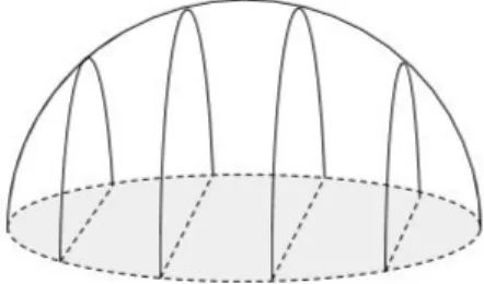
Figure 2.3: Unit disk to hemisphere. Continuity, Connectedness & Compactness
Continuity is an important concept in many areas of mathematics and topology is the right setting for studying it. Several things depend on continuity, but first things first, we begin with the definition.
Definition 2.2.14. Let (X, TX)and (Y, TY)be topological spaces. A function
f : X ! Y is continuous if for every A 2 TY, f 1(A)2 TX.
This is equivalent to saying that for each x 2 X, given a neighborhood Nf (x)
in TY, there is a neighborhood NX in TX such that x 2 NX which belongs to
the preimage of Nf (x). The inverse is given by f 1(A) ={x 2 X : f(x) 2 A}.
Remark. We do not require f 1 to be a function, and in general, it is usually
not one.
Example 2.2.15. The function f : R2
\ {(0, 0)} ! S1, given by f(x) = x kxk,
is continuous. The inverse of f does not exist.
Example 2.2.16. Let f be a vertical projection from the open unit disk to the open hemisphere, see Figure 2.3. Then f : (x, y) ! (x, y,p1 x2 y2), is a
continuous function, as is f 1.
Leaving continuity, our next step is connectedness. It is quite intuitive what connectedness is: connected spaces are in some sense "stuck together" - we could say that from any point in the set you can reach any other without ever leaving the set.
Definition 2.2.17. A topological space X is connected if X cannot be written as a union of two non-empty disjoint open sets.
We need to take care when applying this definition. All possible divisions of the space must be considered otherwise there is a possibility that a "gap" is hidden in one of the two open sets.
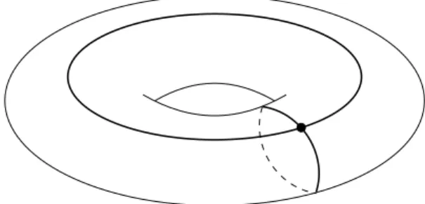
Example 2.2.18. The open interval ( 1, 1) is connected, as is the torus (Figure 2.4), the sphere and the ball.
Example 2.2.19. (R, ¯T) is connected but (R, ˆT) is not since the latter can be written as the disjoint union ( 1, 0) [ [0, 1).
The following theorem ties together the concepts of continuity and connect-edness.
Theorem 2.2.20 (cf. [11]). Let X and Y be topological spaces and f : X ! Y a continuous function onto Y. If X is connected, then Y is connected.
Definition 2.2.21. Let A be a subset of a topological space X. An open cover of A is a collection O of open subsets of X so that A lies in the union of the elements of O, i.e.,
A✓ [
O2O
O
A subcover of O is a collection O0✓ O so that A lies in the union of the elements
in O0. A finite cover (or subcover) is a cover O consisting of finitely many sets.
Definition 2.2.22. A topological space X is compact if every open cover of X has a finite subcover.
Example 2.2.23. The n-sphere is compact for n 2 N. Any finite topological space is compact, such as the spaces in Example 2.2.6.
Example 2.2.24. An infinite set with the discrete topology is not compact. To conclude this part we will state two theorems concerning the compact-ness of subsets, and the connection between continuous functions and compact spaces. Thereafter we will move on to new ways of constructing spaces by using products and quotients.
Theorem 2.2.25 (cf. [11]). If X is a compact topological space and A is a closed subset of X then A is compact.
Theorem 2.2.26 (cf. [11]). Let X be a compact topological space and f : X ! Y a continuous function from X onto a topological space Y . Then Y is compact.
Figure 2.4: Torus: S1
⇥ S1.
Product & Quotient Spaces
This subsection starts by looking at the product of spaces and then it moves on to the quotients of spaces. The reader will have used the concept of a product space many times but perhaps without calling it so. For instance, R3 is the
(Cartesian) product R ⇥ R ⇥ R. By taking the product of spaces we can create new, interesting, topological spaces for us to study.
Definition 2.2.27. Let X be a topological space with topology T and Y a topological space with topology T0. A basis for the product topology on X ⇥ Y
is given by B where N 2 B if N is on the form N = O ⇥ O0 for O 2 T and
O0 2 T0. Projection functions p
X : X⇥ Y ! X and pY : X⇥ Y ! Y are
defined by
pX(x, y) = x
pY(x, y) = y.
pX and pY are continuous and X ⇥ Y is called a product space.
Example 2.2.28. If we take a circle, S1and an interval [a, b] ⇢ R, the product
will be a closed cylinder. The product of two circles, S1
⇥ S1, is a torus (see
Figure 2.4).
For product spaces in general we have that for given X = QXi and fi :
X ! Xi, the product topology is the minimal topology on X that makes all
fi continuous. Two valuable results about product spaces are that the
prod-uct of connected topological spaces is connected, and the prodprod-uct of compact topological spaces is compact.
With product spaces and continuity we can study continuous deformation from one function to another. Imagine the function f0(x) = 2sin(x), if you
10sin(x). We say that two functions are homotopic if one can be continuously transformed into the other. Formally we take the following definition.
Definition 2.2.29. Let X and Y be topological spaces and I = [0, 1]. Then H : X ⇥ I ! Y , given by H(x, t) = Ht(x) for x 2 X and t 2 I, is a
homotopy between the continuous functions f0: X ! Y and f1: X ! Y if
H continuous and satisfies
H(x, 0) = f0
H(x, 1) = f1.
Remark. It is important that the reader observes the fact that all Ht(x) are
required to be continuous for t 2 I.
Example 2.2.30. In topology one usually talks about spaces being "elastic", we can now describe stretching in terms of homotopy. Take R2 and stretch it
out so that each point is sent twice as far away from origo. We can construct a continuous function H : R2⇥ I ! R2 given by
H(x, 0) = H0(x) = x
H(x, t) = Ht(x) = (1 + t)x
H(x, 1) = H1(x) = 2x.
H is a homotopy between H0 and H1.
Now we move on to quotient spaces. Similarly to product spaces, quotient spaces will yield new spaces for us to study. They occur when we identify (or glue together) certain points in a space. If you would, for example, take the boundary of a disk to a single point (without shrinking the surface area), the result will be a sphere. We start with the definition of a quotient topology before we define a quotient space (also known identification space).
Definition 2.2.31. Let (X, T) be a topological space and let f : X ! Y be a function onto the set Y . Define the quotient topology T0 on Y by defining
U ✓ Y to be open in Y if
U 2 T0 iff f 1(U )
2 T
together to form a cylinder. This is the same as saying that the points on one edge are equivalent to those on the other.
Example 2.2.33. Let X be a topological space with ⇠ an equivalence relation defined on X. The equivalence class of x 2 X is given by
[x] ={y 2 X : y ⇠ x},
and the identification space X/ ⇠ is the set of equivalence classes of the relation ⇠, equipped with the quotient topology:
X/⇠ = {[x] : x 2 X}.
The topology on X induces a topology in X/ ⇠. This is the quotient topology from Definition 2.2.31.
Example 2.2.34. To formalize Example 2.2.32; let X = {(x, y) : 0 x 1, 0 y 1} and form the equivalence classes
[(x, y)] = (
{(x, y)} if x 6= 0, 1 and 0 y 1, (0, y)⇠ (1, y) if x = 0, 1 and 0 y 1. Then X/⇠ becomes the cylinder.
2.2.2 Homeomorphisms
Now we shall look at an updated version of the definition of homeomorphisms that was discussed in the beginning. Homeomorphisms gives us topologically equivalent spaces. It is thanks to the following definition that we can bend and stretch spaces and still view them as "the same space".
Definition 2.2.35. A function f, between topological spaces X and Y , is a homeomorphism if f is continuous and invertible and the inverse function f 1
is also continuous. The spaces X and Y are then topologically equivalent, also called homeomorphic, denoted X ⇠= Y.
The examples in Figure 2.1 are homeomorphic. Other examples are stretch-ing one open interval in R to any other, and the very famous one of the torus which is homeomorphic to a coffee mug.
Homeomorphisms help us find unique properties that remain unchanged when during a continuous transformation. These properties lie "deeper" in the structure of the spaces and are therefore interesting to study. What char-acteristics can be found and how can two spaces be differentiated from one another?
Example 2.2.36. The stereographic projection S : S3\ {N} ! R3is a
home-omorphism. Therefore the 3-dimensional sphere (P4
i=1x2i = 1) minus the north
pole, is the same space as R3.
Make the projection by sending a point P = (x1, x2, x3, x4) on the sphere
to a point P0 = (x, y, z, 0) 2 R3 as follows: draw a line from the north pole
N = (0, 0, 0, 1)of the sphere through P . This line is given by (t) = (0, 0, 0, 1) + (x1, x2, x3, x4 1)t
and it intersects R3 when 0 = 1 + (x
4 1)t() t = (1 x4) 1. S can now be written as S(P ) = ((1 x4) 1) = ⇣ x1 1 x4 , x2 1 x4 , x3 1 x4 ⌘ . S is continuous, invertible and has a continuous inverse given by
S 1(P0) =⇣ 2x µ + 1, 2y µ + 1, 2z µ + 1, µ 1 µ + 1 ⌘ , where µ = x2+ y2+ z2. S is therefore a homeomorphism, and S3/
{N} ⇠=R3.
(a) Rectangle (b) Twist (c) One half twist (d) Three half twists
Figure 2.5: Möbius strip.
Example 2.2.37. This example is taken from Armstrong’s book Basic Topol-ogy [2]. It is meant to illustrate that homeomorphisms are more than just stretching and bending. Hence, we cannot only think about topological spaces as being made of rubber. To, for example, construct a Möbius Strip, one starts with a rectangle that has 2 directed edges, as in Figure 2.5a, then identify the edges along the specified direction. In order to do so we induce a half twist,
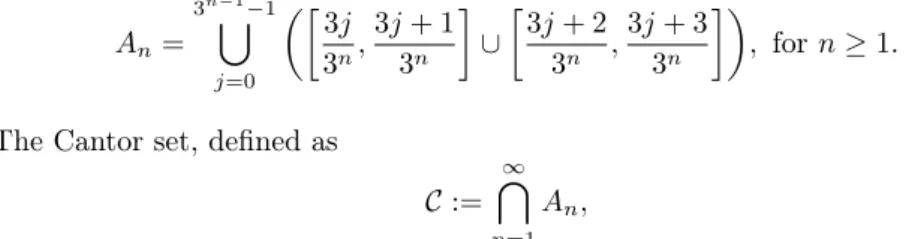
Figure 2.6: Cantor set binary tree - by Sam Derbyshire [16].
Figure 2.5b and 2.5c. However, nothing stops us from adding more twists. As long as we identify the edges according to the directions the same points on both edges will be made to coincide. This always gives an odd number of half twists. So all sub-figures in Figure 2.5 are homeomorphic.
Example 2.2.38. The famous Cantor set is constructed by iteratively removing the open middle third of line segments. Start with A0= [0, 1], which is compact,
remove the middle third and obtain A1= [0,13][ [23, 1], which also is compact.
Again, remove the middle thirds and obtain A2 = [0,312][ [322,332][ [362,372][
[8
32, 1]. Repeating this process gives
An= 3n[1 1 j=0 ✓3j 3n, 3j + 1 3n [ 3j + 2 3n , 3j + 3 3n ◆ , for n 1. The Cantor set, defined as
C :=
1
\
n=1
An,
is a compact set. Look at Figure 2.6, in black we can see the first steps (A0
to A5) in the construction of C. In red we can see a binary tree forming. In
fact: each point in the Cantor set is determined by a unique (infinite) binary sequence. This means that there is a bijection from C to all infinite binary sequences.
Let 2 denote the topological space {0, 1} with the discrete topology. From this we can create the space
of all infinite binary sequences with the product topology of the discrete topology in {0, 1}. By choosing 0 to represent the left interval and 1 to represent the right interval in each step of the Cantor set construction we can form a sequence (represented by the binary tree shown in Figure 2.6) that can uniquely lead us to a point in C. It sounds plausible that 2N is homeomorphic to C, which in
fact it is. To prove this it is common in the literature to take the route through ternary expansions, but there is an approach closer to the material in this thesis which uses binary expansion and the Cantor Intersection Theorem to construct a homeomorphism between C and 2N. The reader is referred to Landstedt’s
publication [12] for the details.
Concepts Depending on Homeomorphisms
The reader will notice that almost everything from now on will depend on homeomorphisms. Homeomorphisms are the foundation for the next chapter on homology, as well as the basis for the entire study of knots. Even so, this chapter will end with a few key concepts that are directly dependent on homeomorphic functions.
Homotopy has previously been defined (Definition 2.2.29) and an example of a dilation of R2was given. If we put an additional requirement on the functions
we get the following definition.
Definition 2.2.39. Let X and Y be topological spaces. A function H : X ⇥ I ! Y is an isotopy if H is a homotopy and each Ht(x)is a homeomorphism.
Demanding homeomorphic functions means that we not only need contin-uous functions (as for homotopy) but also contincontin-uous inverses. Again, looking back to Example 2.2.30. Stretching R2 has a logical inverse in shrinking it. It
is common that to take ˆH0= Id (the identity).
Example 2.2.40. From Example 2.2.30 we have a homotopy H : R2
⇥I ! R2.
We can construct the following function for x 2 R2and t 2 I: ˆH :R2
⇥I ! R2, where H0(x) = x Hˆ0(x) = x Ht(x) = (1 + t)x Hˆt(x) = 2 t 2 x H1(x) = 2x Hˆ1(x) = 1 2x.
space such that every point has a neighborhood homeomorphic to an open n-ball in Rn.
Definition 2.2.43. An n-manifold with boundary is a topological space such that every point has a neighborhood homeomorphic to either an open n-ball in Rn or half of an open n-ball: {x 2 Rn:Px
i< 1, x1 0}.
By surface we will mean a 2-manifold. Surfaces with boundary will be an important part of our study of knots later, but for now we will just give a few examples. Boundary basically means that if you travel along the space you can come to a verge where you can "fall off" if you cross it.
Example 2.2.44. The sphere, torus, Klein bottle and the projective plane are all 2-manifolds. The punctured sphere (disk), punctured torus, a sheet of paper, and the Möbius band are 2-manifolds with boundary.
In this chapter we will take a different approach - to study building blocks that together make up spaces. These blocks are called cells and cells can be glued together to form complexes. The essence of this chapter is to create algebraic structures that can help us distinguish different objects (spaces) from each other by identifying properties that are unique to each object. This chapter follows the excellent books of Armstrong [2], Fulton [5], and Kinsey [11].
3.1 Complexes
Definition 3.1.1. An n-cell is a is a set whose interior Int( ) is homeomor-phic to an open ball, with the additional property that its boundary must be divided into a finite number of lower-dimensional cells, called the faces of the n-cell. We write ⌧ < if ⌧ is a face of .
Example 3.1.2. For this example we will restrict ourselves to cells called sim-plexes, these are n-dimensional generalizations of triangles, see Figure 3.1.
1. A 0-simplex is a point A.
2. A 1-simplex is a line segment a = AB, and A < a, B < a.
3. A 2-simplex is a triangle, such as = ABC, and then AB, BC, AC < . Note that A < AB < , so A < .
4. A 3-cell is a tetrahedron, with triangles, edges, and vertices as faces. Connecting back to all cells, notice from the definition that there are no requirements for a 1-cell to be a straight line, it suffices that its interior is
A (a) 0-simplex B A a (b) 1-simplex C A B (c) 2-simplex D C B A (d) 3-simplex
Figure 3.1: Examples of simplexes.
homeomorphic to ( 1, 1). A 2-cell is not necessarily a triangle rather its interior will be homeomorphic to an open 2-dimensional disk, and similarly for any n-cells.
The faces of an n-cell are cells of lower dimension. With these cells one can construct new objects: e.g., take a point, 0-cell, attach a 1-cell (string) to the point so it forms a loop, and then attach a 2-cell (surface) to the string. This might look a like flat disk with a marked edge and a point on the edge. This type of construction forms something called a complex - a union of cells that follow certain rules.
Definition 3.1.3. A complex K is a finite set of cells, K =[{ : is a cell} such that:
1. if is a cell in K, then all faces if are elements of K; 2. if and ⌧ are cells in K, then Int( ) \ Int(⌧) = ;.
The dimension of K is the dimension of its highest-dimensional cell.
Remark. The second rule in the definition stops cells from overlapping or cross-ing each other. Cells can only meet at their boundary, i.e. they can share faces.
If a complex is constructed using only simplexes (the very nice cells that were shown in Example 3.1.2), we call it a simplicial complex. Simplexes usually make calculations more straightforward but also more tedious. Even if they are special cases of cells one does not lose any information when using them [6], and they are therefore very common in the literature.
Instead of giving instructions for how each cell should be glued together to form a complex we will represent complexes though planar diagrams. This means that we take a 2-dimensional disk and mark which cells are supposed to be glued together, as the examples in Figure 3.2. These show the four ways of gluing the sides of a square to form a surface, (a) the sphere, (b) the torus, (c) the Klein bottle, and (d) the projective plane.
Q P Q R a a b b (a) S2 P P P P b a b a (b) T2 P P P P b a b a (c) K2 Q P Q P b a b a (d) P2
Figure 3.2: Four surfaces: sphere, torus, Klein bottle, and projective plane. Definition 3.1.5. The space underlying a complex K, or the realization of K, is the set of all points in the cells of K;
|K| = {x : x 2 2 K, a cell in K}, where x belongs to any ambient space.
So, what is the difference between a complex and a space? Well, a complex is a set of cells of various dimensions, while a space is a set of points. This means that |K| is a space and K are the building blocks of that space.
There are many different ways to assign a complex to a space. Therefore, in examples we will not give a complex its own name (i.e. K) but rather use the notation of the space (i.e. S2) to mean the complex on that space. This
is to emphasize that it is the structure of the space |K| and not the complex itself that is important. By n-complex we will mean a complex K with cells of dimension n or lower, e.g. a 2-complex can only consist of 0-, 1-, and 2-cells.
The following definition is a special case of a complex, namely a simplicial complex on a surface consisting of only 2-simplexes.
Definition 3.1.6. A surface (with or without boundary) is triangulable if a simplicial 2-complex K can be found with X = |K| and the 2-simplexes (or tri-angles) of K satisfy the additional property that any two triangles are identified along a single edge or a single vertex or are disjoint.
This definition deals with surfaces we divide into (or construct by) triangles (2-simplexes). We call these surfaces triangulable and we will base some of our study of knots on surfaces with this property.
3.2 The Algebra of Chains
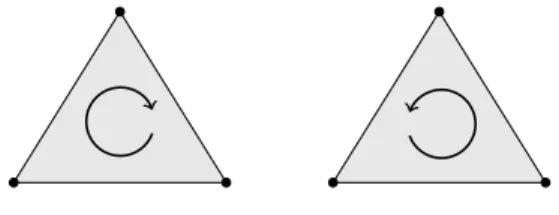
In the previous section we gave 1-cells directions to elucidate which sides to glue together in the planar diagrams. Now we will use the fact that all cells can be given a orientation, see Figure 3.3, to form what is known as directed complexes.
Figure 3.3: Orientations of 2-cells.
Giving a cell an orientation is the equivalent of saying if one is using the right-handed or the left-right-handed orientation of the basis in Euclidean three-space. Definition 3.2.1. An n-cell is oriented if it has been assigned one of the two orientations: positive ( ) or negative ( ).
The choice of which orientation is positive and negative is arbitrary. The orientation of an n-cell induces an orientation on its faces.
Definition 3.2.2. An n-complex is directed if all cells of dimension 1 or higher have been given an orientation.
Example 3.2.3. A 2-complex K is directed if each edge or 1-cell is given an orientation (from initial to terminal point) and each polygon or 2-cell is given an orientation (clockwise or counterclockwise).
In a directed complex the choice of orientation of the cells is arbitrary. It serves as a basis for calculations. If two cells share a face and the orientation of cells match up, the face can be removed without affecting the complex because
orientation on the edges c, d, and e). If all adjacent cells in a complex have compatible orientation we call the underlying space orientable.
Example 3.2.4. A surface is orientable when it is 2-sided, like the sphere and torus but unlike the Möbius strip and the Klein bottle. We will return to the concept of orientable surfaces in the chapter about knot theory.
Definition 3.2.5. Let K be a directed complex. An (integral) k-chain C in K is a formal sum
C = a1 1+ a2 2+ ... + an n
where 1, 2, ..., nare k-cells in K and a1, a2, ..., anare integers. Define 0 = 0.
Definition 3.2.6. Let C =Pn
i=1ai iand DPni=1bi ibe k-chains in a directed
complex K. The sum C + D is defined by
C + D = (a1+ b1) 1+ (a2+ b2) 2+ ... + (an+ bn) n.
Remark. In addition to this definition we need to specify that 0 is a k-chain for each value of k.
This is a very intuitive definition, but a short example is in order. Let C = d + 2eand D = 3c 2d + e be q-chains in a directed complex, then
C + D = (d + 2e) + (3c 2d + e) = 3c d + 3e.
This definition, addition of k-chains, have the normal properties one usually associates with addition; commutativity, associativity and the existence of both identity and inverse. One adds chains of the same dimension.
Definition 3.2.7. Let K be a directed complex. Denote the group of all k-chains on K, with addition, by Ck(K), k = 0, 1, ..., dim(K).
Ck(K)is the kth chain group of K. Ck(K)is an abelian group: the addition
satisfies the definition and all chains in Ck(K)are k-dimensional so adding them
will only yield new k-chains. Ck(K) is generated by the oriented k-cells of K.
If K is a finite complex, Ck(K) will be the free abelian group isomorphic Zn,
for some n.
The following examples specify all chain groups for two different complexes, one on the sphere and the other on the Klein bottle.
Example 3.2.8. Look at the complex on the sphere in Figure 3.2. The 2-cell has no given name or orientation, call it and give it the clockwise orientation. Denote the whole complex K. Now we can calculate all the chain groups. The complex is constructed from three 0-cell: P, Q, and R, two 1-cells: a and b, and one 2-cell: . C0 is the group of all 0-chains on S2. That means that all linear
combinations of P, Q and R are, such as 3P + 2Q R, belong to C0.
C0(S2) ={n1P + n2Q + n3R : ni2 Z} = hP, Q, Ri ' Z Z Z = Z3
C1(S2) ={;, a, a, ..., b, b, ..., a + b, a b, 3a + 4b, ...} =
={n1a + n2b : ni2 Z} = ha, bi ' Z Z = Z2
C2(S2) ={n : n 2 Z} ' Z
Example 3.2.9. Look at the complex on the Klein bottle shown in Figure 3.4. It has two 0-cells: {P, Q}, five 1-cells: {a, b, c, d, e}, and three 2-cells: { , ⌧, ⇢}.
C0(K2) ={a1P + a2Q : ai2 Z} ' Z2 C1(K2) ={a1a + a2b + a3c + a4d + a5e : ai2 Z} ' Z5 C2(K2) ={a1 + a2⌧ + a3⇢ : ai2 Z} ' Z3 P P P P Q b a b a c d e ⌧ ⇢ Figure 3.4: A complex on K2.
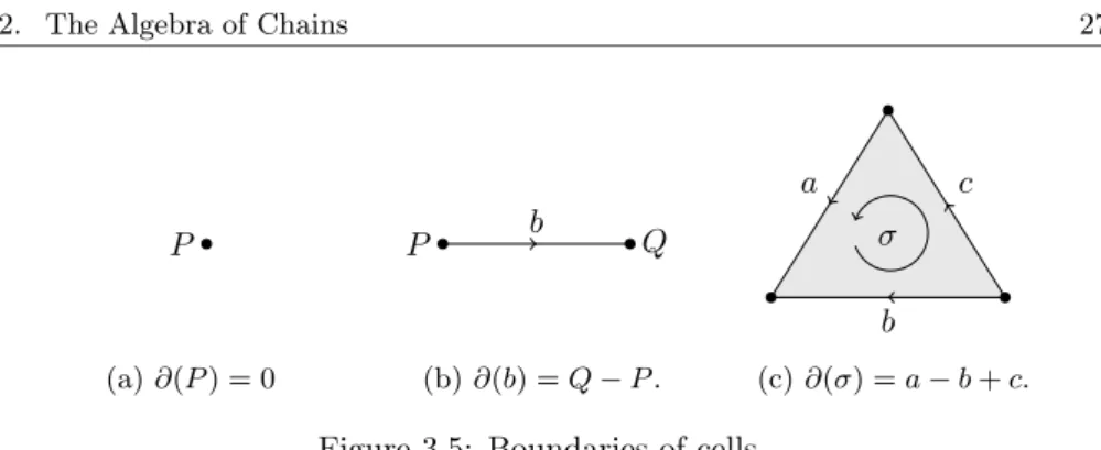
Definition 3.2.10. The boundary of a k-cell , denoted @( ), is the (k 1)-chain consisting of all the (k 1)-cells that are faces of , with orientation inherited from the orientation of .
Figure 3.5 shows some examples of boundaries for different k-cells. For a 0-cell P we define the boundary, @(P ) = 0. For the directed 1-0-cell b the boundary is defined as the terminal point minus the initial point, i.e., @(b) = Q P . The last one, 3.5(c), is an oriented 2-cell , whose boundary is a chain of 1-cells. The 1-cells a, b and c are positive if their directions are consistent with ’s and negative if not. Hence, for 3.5(c), we get the boundary @( ) = a b + c
(a) @(P ) = 0 (b) @(b) = Q P .
b
(c) @( ) = a b + c.
Figure 3.5: Boundaries of cells.
Definition 3.2.11. Let C be a k-chain, C = a1 1+ a2 2+ ... + am m. The
boundary of C is
@k(C) = a1@( 1) + a2@( 2) + ... + am@( m).
So, @k is a function that takes a k-chain and returns a (k 1)-chain, @k :
Ck(K) ! Ck 1(K). The boundary function @k is a homomorphism, since, if
Cand D are both k-chains, then @k(C + D) = @k(Pni=1(ai+ bi) i) =Pni=1(ai+
bi)@k( i).
Example 3.2.12. Let C be the 2-chain 2⌧ 3⇢ from the complex in Figure 3.4. Then the boundary of C is
@2(C) = 2@(⌧ ) 3@(⇢) = 2(b c + e) 3(b + c + d a) = 3a b 5c 3d + 2e.
Can we conclude something from this 1-chain that is the boundary? In this particular case there is not much to say, however, there is a special case when this boundary function gives rise to something interesting. Take another look at Figure 3.4. The boundary of b is P P = 0. The same is true for @(a d e) = 0. So, what does it mean when the boundary terms of a chain cancel out? Well, it means that we have found a cycle!
Definition 3.2.13. If C is a k-chain in a directed complex K s.t. @k(C) = 0,
we say that C is a k-cycle. The set of all k-cycles in K, Zk(K), is a subgroup
of Ck(K).
Remark. Zk(K) is also the kernel of @k : Ck(K)! Ck 1(K).
Definition 3.2.14. If C is a k-cycle in a directed complex K such that there exists a (k + 1)-chain D with @k+1(D) = C, we say C is a k-boundary. The set
of all k-boundaries in K is Bk(K)✓ Ck(K).
Not only is Bk(K) a subgroup to Ck(K) in fact it is true that Bk(K) ✓
Zk(K)✓ Ck(K). This is a consequence of the following theorem.
Theorem 3.2.15 (cf. [2]). The composition @k+1 @k : Ck+1 ! Ck 1 is the
zero homeomorphism.
If you apply the boundary function twice you will always get 0. A proof can be found in [2], but in short this means the the boundary of any cell is a cycle. Example 3.2.16. Let us revisit Figure 3.4 again. In this complex, name the 1-cycle a d e = C1. The definitions says that because the boundary of the
2-chain D1 = is precisely C1, then C1 is called a 1-boundary. The chains
C2 = b c + eand C3= b + c + d aare also 1-boundaries with D2= ⌧ and
D3= ⇢respectively. There exists no 2-boundaries because the complex contains
no 3-cells.
3.3 Homology Groups
In this section we will reach our goal for this chapter - Homology groups. Their definition will be stated first and this whole chapter will be concluded by several examples that give a deeper understanding as well as illustrate why all of this has been worth doing, but first a short recap.
We have constructed chains from cells of the same dimension. On these chains we have defined orientation and boundary and noticed that chains with null-boundary form some kind of loop that we can think of as enclosing a k-dimensional hole. By studying sets of cycles we will distinguish spaces based on what type of cavities they have. For example, the normal sphere encloses a 3-dimensional cavity, as does the torus, but when we at the end of this section look at the combined picture, over all dimensions, we will be able to tell them apart. Homology groups Hk(K) are used to describe structures in different
dimensions. One can think of them as follows:
H0(K)describes the connectivity of the components,
H1(K)describes non-trivial loops, i.e. holes that look like a circle,
H2(K)describes holes which look like a sphere,
...
Definition 3.3.1. Let K be a directed complex. The kth homology group of K is Hk(K) = Zk(K)/Bk(K) =h ¯k, k2 Zi, the group of equivalence classes
of elements of Zk(K) with the homology relation. In other words, Hk(K) is
Definition 3.3.2. The k-chains C1 and C2 are homologous, written C1⇠ C2,
if C1 C22 Bk(K); i.e., if C1 C2= @(D)for some (k + 1)-chain D.
Example 3.3.3. From Figure 3.5b, c: @(b) = Q P () P ⇠ Q therefor Q is in ¯P, and @( ) = a b + c () a + c ⇠ b, so a + c 2 ¯b.
Example 3.3.4. A few examples from Figure 3.4: • @(a) = P P () P ⇠ P , naturally,
• @(c) = Q P () Q ⇠ P ,
• @(⌧) = b + e c() b + e ⇠ c, or b + e 2 ¯c and
• @(⇢) = b a + c + d() a b⇠ c + d () a b2 ¯c + d.
Theorem 3.3.5 (cf. [11]). Let K be a complex, with C1, C2, C3, C4 chains in
Ck(K):
1. C1⇠ C2.
2. If C1⇠ C2, then C2⇠ C1.
3. If C1⇠ C2 and C2⇠ C3, then C1⇠ C3.
4. If C1⇠ C2 and C3⇠ C4, then C1+ C3⇠ C2+ C4.
Remark. This theorem shows that homology is an equivalence relation and that it works well with the chain addition (4).
Below are step-by-step directions for how to compute Hk(K). These seem
tedious and take a bit of practice to get the hang of. A reminder about notation: the trivial group is denoted by e0.
Step-by-step Directions. First label and indicate orientation of all cells of the complex. Do the computations for one dimension at a time, starting with the highest.
1. Find Ck(K), the group of all k-chains.
2. For each generating k-chain C from (1), compute @(C). 3. Find Zk(K), using your computations from (2).
(a) Note that if Zk(K) = e0, then Hk(K) = e0.
(a) When working in the highest dimension, note that Bk(K) = e0, since
there are no (k+1)-chains for which the k-chains can form boundaries. (b) Otherwise, look back to (2) in the next highest dimension, where you
already computed which k-chains are boundaries of (k + 1)-cells. (c) Note that if Bk(K) = e0, then Hk(K) = Zk(K).
5. Compute Hk(K), by taking Zk(K) from (3) and using any homologies
found in (4).
Let’s go through a few examples.
Example 3.3.6. We have already worked with the sphere in Figure 3.2a, now it is time to compute its homology groups. Call the 2-cell and give it a clockwise orientation. There are no cells of higher dimension than 2, therefore Hk(S2) = e0, for k > 2.
H2(S2) :
1. There is only one 2-cell: , therefore C2(S2) =h i ' Z.
2. @( ) = a a + b b = 0. This means that is a 2-cycle.
3. The 2-cycle generates the whole group of 2-cycles: Z2(S2) =h i ' Z.
4. Because there are no 3-cells B2(S2) = e0.
5. We get that H2(S2) = Z2(S2)' Z.
H1(S2) :
1. There are two 1-cells: a and b, therefore C1(S2) =ha, bi ' Z Z.
2. @(a) = P Q6= 0, @(b) = R Q6= 0. Neither a nor b are 1-cycles. The only 1-cycle is the trivial 0.
3. So Z1(S2) = e0.
4. The only 1-chain that is a 1-boundary (bounds ) is 0 = a a + b b, therefore B1(S2) = e0. 5. We get that H1(S2) = e0. H0(S2) : 1. C0(S2) =hP, Q, Ri ' Z3 2. @(P ) = @(Q) = @(R) = 0 3. Z0(S2) =hP, Q, Ri ' Z3
4. From the calculations of H1(S2), step 2, we have that P ⇠ Q ⇠ R because
@(a) = P Q6= 0, @(b) = R Q6= 0.
5. Combining Z0(S2)with the homology relations (Q, R are in ¯P) from step
1. There is only one 2-cell: , therefore C2(T2) =h i ' Z.
2. @( ) = a + b a b = 0. This means that is a 2-cycle.
3. The 2-cycle generates the whole group of 2-cycles: Z2(T2) =h i ' Z.
4. Because there are no 3-cells B2(T2) = e0.
5. We get that H2(T2) = Z2(T2)' Z.
H1(T2) :
1. There are two 1-cells: a and b, therefore C1(T2) =ha, bi ' Z Z = Z2.
2. @(a) = @(b) = P P = 0. Both a and b, and any linear combination of them, are 1-cycles.
3. The 1-cycles a and b generate the group of 1-cycles: Z1(T2) =ha, bi ' Z2.
4. The only 1-chain that is a 1-boundary (bounds ) is 0 = a + b a b, therefore B1(T2) = e0. 5. We get that H1(T2) = Z1(T2)' Z2. H0(T2) : 1. C0(T2) =hP i ' Z 2. @(P ) = 0 3. Z0(T2) =hP i ' Z
4. From the calculations of H1(T2), step 2, we have that @(a) = @(b) =
P P = 0. Which gives us that B0(T2) = e0.
5. Thus H0(T2) = Z0(T2)' Z.
Example 3.3.8. Take a look at the complex in Figure 3.6. Call this complex K. Observe that forms a sphere and that there are no cells of dimension 3 or higher.
H2(K) :
1. and ⌧ are the only 2-cells and they generate the group of all 2-chains; C2(K) =h , ⌧i ' Z2.
2. @( ) = 0 and @(⌧) = f + g e, so is a 2-cycle. 3. The group of 2-cycles is Z2(K) =h i ' Z.
v1 v2 v3 v4 v5 v6 v7 a a d b c e f g ⌧
Figure 3.6: Complex K for Example 3.3.8. 5. H2(K) = Z2(K)/B2(K) = Z2(K)' Z.
H1(K) :
1. There are seven 1-cells; a, ..., g. These generate the C1(K), so C1(K)' Z7.
2. @(d) = @(f + g e) = 0, so d and f + g e(and any multiple of these) are the only 1-cycles.
3. Z1(K) =hd, f + g ei ' Z2
4. Homology relations
• From 2. we get that e ⇠ f + g. f + g eis a 1-boundary because it is the boundary of a 2-chain i.e. ¯e is one of the generators of B1(K).
• Looking at d we see that it is not the boundary of any 2-chain hence ¯
dis not a generator for B1(K).
• B1(K) =h¯ei ' Z. 5. This gives us H1(K) =h ¯di ' Z. H0(K) : 1. C0(K) =hv1, ..., v7i 2. @(vi) = 0, i ={1, ..., 7} 3. Z0(K) =hv1, ..., v7i ' Z7
4. From the calculations of H1(K), step 2, we have that v1⇠ v2⇠ v3 ⇠ v4
and v5 ⇠ v6 ⇠ v7, so there are only two equivalence classes ¯v1 and ¯v5.
B0(K) =hv1 v2, v1 v3, v1 v4, v5 v6, v5 v7
5. Combining Z0(K)with the homology relations found in step 4 gives H0(K) =
h ¯v1, ¯v5i ' Z2.
Thees homology groups have given us the information that the complex has two connected components, one cavity similar to a sphere, and another cavity similar to a circle. The rest of the structure is disregarded, it does not add new information. We regard all structures containing two components, one circle, and one sphere, as the same.
A powerful result is the fact that the homology groups obtained in simplicial homology actually coincides with the homology groups we have obtained. This is however not an easy feat to prove and the interested reader is refereed to [6] for a detailed account.
We will end this chapter by building a bridge into knot theory. In knot theory we will make use of something called polyhedral surfaces.
Definition 3.3.9. A polyhedral surface is a triangulable surface (or 2-manifold) possibly with boundary.
If we can construct a surface (with or without) boundary from triangles or 2-simplexes, following the rules of triangulation, we call this a polyhedral surface. A cylinder is an easy example of a polyhedral surface. Viewing the cylinder as a rectangle and imagine dividing the rectangle into two triangles gives a triangulation of the cylinder. By having complexes on a surface we know that there are tools that help us study these surfaces. In the chapter on knot theory the boundary of a surface will be the most important part, as it is actually a knot, and the techniques developed in this chapter will allow us to study the knot using this surface, but more on that later.
Orientation has been mentioned earlier and the following definition agrees with the one previously given but is stated only for polyhedral surfaces. Definition 3.3.10. A polyhedral surface is orientable if it is possible to orient each triangle in such a way that that when two triangles meet along an edge, the two induced orientations run in opposite directions.
For polyhedral surfaces to be oriented we need that when two triangles are glued together along an edge the induced orientations on the edge run in opposite directions and therefore cancel out.
Definition 3.3.11. The Euler characteristic for a polyhedral surface S with a triangulation consisting of F triangles, E edges and V vertices, is given by
(S) = F E + V.
The Euler characteristic is defined for simplexes but in fact we can use any complex on a triangulable surface to calculate it if we let F be 2-cells, E be 1-cells and V be 0-1-cells. This follows from the fact that homology and simplicial homology are equivalent.
Example 3.3.12. We have previously worked with the complexes in Figure 3.2, let us do so again. Both the sphere S2 and the torus T2 are triangulable
and orientable. From the complexes in the figure we have that (S2) =1 2 + 3 = 2
(T2) =1 2 + 1 = 0
The reader can check that if a triangulation on the sphere is constructed, by adding say a 1-cell connecting P and R, the Euler characteristic does not change. Neither does adding a diagonal 1-cell in the complex on T2.
We have now studied both homology groups and the Euler characteristic and with the help of Betti numbers, see below, we will combine them. The Betti numbers are topological invariants that aid us in our study of spaces.
Definition 3.3.13. The Betti numbers of a complex K are k = rk(Hk(K)).
Theorem 3.3.14 (cf. [2]). The Euler characteristic of a finite complex K is given by the formula
(K) =
n
X
k=0
( 1)k k,
where n is the dimension of K.
Definition 3.3.15. The genus of a connected orientable surface S is given by g(S) = 2 (S) B
2 ,
where B is the number of boundary components of the surface.
Example 3.3.16. Neither the sphere nor the torus have boundary and therefore g(S2) = 0 and g(T2) = 1. The cylinder on the other hand has boundary, 2
boundary components to be exact, and can be triangulated with two triangles giving it Euler characteristic 0 and genus 2 0 2
In the introduction a knot was described as something that is formed when we take a string, tie it, and then glue the ends of the string together. If you do not attach the ends together the string can be tied and untied over and over again in different ways. In this chapter a mathematical definition of a knot is given and several knot invariants are defined, some more helpful than others. The last two sections are dedicated to two knot polynomials: the bracket polynomial and the Jones polynomial. Both are invariants and have contributed greatly to this field.
4.1 Introduction to Knot Theory
In this secton we follow: [1] [3], [13] and [14]. In this work we study knots that are embedded in S3. One can project a knot onto a plane (or simply draw it
on a paper). These projections are called knot diagrams, see Figure 4.1. To avoid ambiguity there are a few restrictions:
1. At each crossing it is clear which string segment passes over respectively under the other (this is usually done by drawing a gap in the bottom segment).
2. Each crossing involves exactly two segments of the string. 3. The segments must cross transversely.
Some intuitive terminology: At each crossing there is always one over-strand and one underover-strand. An arc is a piece of the knot that passes from one undercrossing to another with only overcrossings in between, i.e., an
Figure 4.1: Figure 8 knot.
Figure 4.2: Knot table - by Wikipedia user Jkasd [22], published with permis-sion.
"unbroken" line in the diagram. We will work extensively with the knot dia-grams but it is important to remember that these diadia-grams are only projections of the knot.
Definition 4.1.1. K is a knot if there is an embedding h : S1 ! S3 whose
image is K. We say that K ✓ S3 is homeomorphic to the unit circle S1
The actual knot is a smooth embedding of the unit circle in S3. The diagrams
are, in fact, sufficient for showing all results that are covered in this work. Why this is true will be dealt with shortly. A knot can only consist of one component, a link on the other hand is a finite union of disjoint knots. Many of the following concepts can be generalized to links.
When studying knots one matter of great importance is being able to tell knots apart (as well as being certain when they are one and the same). It will later be apparent just how hard this actually is. For now you should know that
Figure 4.3: Wild knot - by Wikipedia user Jkasd [21], published with permission. we are able to tell many knots apart, although, there exists no method that can fully distinguish all knots from each other. Finding methods for differentiating knots means finding knot invariants, that is, properties that remain unchanged no matter which projection or embedding of the knot we happen to be studying. We will work our way though several invariants all the way to the famous Jones polynomial which was revolutionary when discovered. To do this we must first specify what is meant by two knots being "the same".
Definition 4.1.2. Knots K1and K2in S3are equivalent if there exist a
home-omorphism h : S3
! S3such that h(K
1) = K2.
We work with knots in the space S3 and we consider two knots to be two
representations of the same knot if there is a homeomorphism of the whole space that takes one representation to the other. A tame knot is a knot that can be constructed with line segments. This ensures that the knots are "nice" to work with, e.g. shrinking a part of the knot to a point is not allowed, neither are knots that need an infinite construction. A knot that is not tame is called a wild knot, see Figure 4.3. All knots in this thesis are tame knots.
Definition 4.1.3. If H is an isotopy between ambient spaces, that is H : S3
⇥ I ! S3, then H is an ambient isotopy.
Ambient isotopy is a stronger requirement than just the existence of a home-omorphism between knot embeddings. By looking at knots from this perspective we can utilize algebraic methods in our study and in fact no information is lost. Even though structure is gained it would still be very tedious and hard work to explicitly construct ambient isotopies between spaces whenever we wish to show that two knots are equivalent. Thankfully this is not necessary. Work done by Reidemeister integrated combinatorial techniques into knot theory and these are very easy to work with. The following definition describes what is called the Reidemeister moves. These operations work with the knot diagrams rather than the actual knot. The pictures in the definition only show a small part of the diagram, the rest remains unchanged.
Definition 4.1.4. The Reidemeister Moves.
R1: ⌦ ⌦
R2: ⌦ ⌦
R3: ⌦
So, what can we do with the Reidemeister moves? Well R1 allows us to remove (or introduce) a twist in a diagram. The result is that the knot will have one fewer (or one more) crossing. R2 lets us separate two strings that lie on top of each other or vice versa. This will add or remove two crossings. R3 allows us to move a strand from one side of a crossing to the other. This also works if the strand being moved is above the other two strands. R3 does not affect the number of crossings in the current projection. If a deformation of the diagram only uses R2 and R3 we call this a Regular isotopy (or planar isotopy). A word of caution: regular isotopy is an equivalence relation for the knot diagrams and is not defined for the knot embedding.
The Reidemeister moves only describe procedures performed on the dia-grams. It is not intuitively clear that studying knot diagrams is a technique strong enough to allow us to draw conclusions about the actual knot. Fortu-nately it is a very strong technique, which is shown in the following theorem. Theorem 4.1.5 (Reidemeister’s theorem). If two knots K1and K2are ambient
isotopic, then there is a sequence of Reidemeister moves taking a projection of K1 to a projection of K2.
Proof by Kauffman in article [10]. Reidemeister not only defined these moves for knot diagrams he proved that one can, using only R1-R3, always transform two knot projections into one another if and only if they are projections of the same knot.
Example 4.1.6. The knot in Figure 4.4 is equivalent to the unknot. Use the Reidemeister Moves to convince yourself of this.
We are striving to find ways to tell knots apart. It feels intuitively obvious that there exists more knots than just the unknot and with the next result we can show that there exists (at least) two different knots. Another name for the
Figure 4.4: Unknot in disguise.
unknot is the trivial knot, and all knots distinguishable from the unknot are therefore called non-trivial knots.
Definition 4.1.7. A knot diagram is tricolorable if each arc in the knot digram can be assigned a single color such that
1. at least two colors are used, and
2. at each crossing all three incident arcs are either all different colors or the same color.
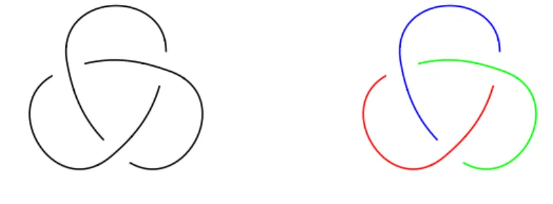
Figure 4.5: Tricoloring of trefoil.
In Figure 4.5 it is shown that the this projection of trefoil knot is tricolorable. Theorem 4.1.8 (cf. [14]). If a diagram of a knot, K, is tricolorable, then every diagram of K is tricolorable.
Proof. (Outline) By tricoloring the Reidemeister Moves one can see that they do not affect the color of the rest of the diagram. This means that they cannot alter tricolorability for a knot diagram, and hence, if one diagram is tricolorable all are.
This makes tricoloring a knot invariant. The unknot is not tricolorable, thus it is different from the trefoil. In the knot table, Figure 4.2, only knots 31, 61,
74and 77can be colored. Observe that we cannot yet distinguish the colorable
(or uncolorable) knots from each other, at the moment we can only be certain that there exists two different knots - the trivial and a non-trivial.
The knots in the knot table, Figure 4.2, are labeled in the Alexander-Briggs notation. This organizes knots based on their crossing number, the subscript is just a counter to separate knots with the same crossing number.
Definition 4.1.9. The crossing number, c(K) of a knot K, is the minimum number of crossings that occur in any diagram of K.
Example 4.1.10. For the unknot we have that c(unknot) = 0. The projections of the trefoil seen so far all have 3 crossings, so is c(trefoil) = 3? Yes, it is. Simply because there are no knots such that c(K) = 1 or 2. To show this first draw one crossing and connect the ends in all 4 possible ways: this only yields the unknot. Then draw two crossings and connect the ends in all possible ways: this gives the unknot, two unknots (which is a link), the Hopf link. Therefore 3 is the minimum number of crossings you need to draw the trefoil. The crossing number is not easy to find, you need to prove there are no representations of the knot with fewer crossings, and right now we cannot show that knot 62is in fact
not just a more complex diagram of any of the knots with fewer crossings. We will find a way to do so later. The crossing number for a knot is an invariant, but at the moment not a very helpful one.
Definition 4.1.11. A knot is oriented if it has an orientation assigned to it. This is illustrated by arrows.
Orientation is extra information that can be added to the knot diagram. If a knot K has a given orientation we take K to mean K with reverse orientation. A knot is called invertible if K and K are equivalent. All knots in Figure 4.2 are invertible. The first non-invertible knot is one with eight crossings (817)
[20].
(a) +1 crossing. (b) 1 crossing.
Figure 4.6: Positive and negative crossing.
Definition 4.1.12. The writhe of an oriented knot, w(K), is the sum of the crossings with signs as shown in Figure 4.6.

![Figure 4.2: Knot table - by Wikipedia user Jkasd [22], published with permis- permis-sion.](https://thumb-eu.123doks.com/thumbv2/5dokorg/5406308.138591/48.892.312.595.421.643/figure-knot-table-wikipedia-jkasd-published-permis-permis.webp)