Developing a long-term, high-resolution, continental-scale, spatially distributed time-series of topographically corrected solar radiation
17
0
0
Full text
(2) Hobbins et al.. in ETa in particular, therefore, inputs of QN are necessary that are accurate, spatially flexible, and long-term. The development of a preliminary long-term, large-scale distributed data set of regional ETa [Hobbins et al., 2001b] has demonstrated the efficacy of models of based on Bouchet's [1963] complementary relationship hypothesis and, in particular, their tunability in areas of homogeneous relief [Brutsaert and Stricker, 1979; Morton, 1983; Claessens et al., 1995; Hobbins et al., 2001a; Hobbins et al., 2001b]. However, more questions have been raised about the most appropriate method of enhancing the model in the sub-optimal conditions typified by the rugged western U.S.. In order to do so, the effects of noisy input data must be removed. An a priori assumption in such terrain is that the effects of local topography introduce a significant noise into the signal of the solar radiation budget, if they are not taken into consideration in the spatial interpolation. This noise may be biased, in regions that predominantly face a specific aspect, for instance, or in regions that fall under local shadowing. In the context of this study, direct observations of the effects on ETa of change and variability in the solar radiation balance at the land surface-atmosphere interface demand a more accurate representation of the interaction of solar radiation and local topography. Other studies of trends in the hydrologic cycle have concentrated on the directly observable components of the hydrological cycle; namely precipitation [Karl and Knight, 1998] and streamflow [Wahl, 1992; Chiew and McMahon, 1996; Lins, 1997; Lins and Slack, 1999]. Even those studies that take a more holistic hydrological approach—whether it be an examination of indices of climate change [Karl et al., 1996] or long-term hydroclimatological trends [Lettenmaier et al., 1994] over the conterminous U.S., or of the effects of climate change on the hydrology of a smaller, regional-scale basin [Westmacott and Burn, 1997]—do not examine trends in ETa, or of its radiative budget, QN. When evapotranspiration has been studied, it is in the context of potential evapotranspiration at a point [Lockwood, 1994]—and that often derived from observations at evaporation pans [Eitzinger et al., personal communication, 2001]—and not ETa at a regional scale. More recent and specifically related studies of trends in ETa or of QN have remained station-based [Szilagyi, 2001]. Szilagyi [2001] offers the closest and most recent comparable study on the effects of trends in the components of ETa. They conclude that models based on the complementary relationship overestimate increases in ETa, yet do not examine the effect of their assumption of no long-term change in QN, which would negate this apparent error. With the dataset we propose, we will be able to close this gap, to check for trends in all components of the ETa expression: including QN. Further, while past reliance on station-based, or small-scale estimates avoids issues relating to errors due to spatial interpolation and rugged topography or the combination of both, it does not allow for study of regions outside of cities, or in rugged terrain. In generating large-scale, spatially distributed. 104.
(3) Developing a Long-term, High-resolution, Continental-scale, Spatially Distributed Timeseries of Topographically Corrected Solar Radiation.. estimates of ETa and, therefore, of QN, we aim to do no less than shed light to these dark spots on the hydrologic map. The primary difficulties in generating QN are two-fold: (i) ground-based observations are few and far between, and (ii) such observations as exist are intricate to interpret and difficult to apply, especially in rugged terrain. Observation stations are sparse—at any one time in the last 50 years, there have only been about 50 stations actively measuring solar radiation across the conterminous U.S.. Topography presents its own set of issues, particularly so in the western U.S., specifically the effects of the orientation of the terrain with respect to the normal direct radiation, which themselves vary temporally on diurnal, seasonal, and trans-decadal cycles. In relation to this latter transdecadal cycle, we need many decades of data to ensure that a trend analysis is not simply reflecting the cyclical behavior, or being biased by it. Our need to build long-term data sets raises the need for conflation of data from different sources. Given the unstable nature of the solar radiation recording network across the conterminous U.S., we must resolve the issue of rebuilding a gappy data set by stitching data sets together and filling in gaps. Having here motivated this study, the following section summarizes the role of QN in hydrologic cycle, specifically in the energy budget of an evaporating surface, and describes the gathering and infilling of the data sets used. The meat of the paper follows, in the description of the breakdown of QN into its component radiations—direct normal radiation (RD) and horizontal diffuse radiation (RH), the analysis of the effects of variable solar geometry, and the development of a correction factor that both adjusts for topography and accounts for the various temporal solar cycles outlined above. Preliminary results of this analysis are shown in the form of surfaces of mean annual QN and annual trends in RT over the conterminous U.S. at a spatial resolution of 5-km for the period WY 1953-1994. Then the preliminary conclusions of this study, their implications, and the further work necessary to complete the development of the dataset are discussed. 2. Methodology This section of the paper proceeds from a general examination of the surface energy budget, deriving QN—net surface radiation or the energy available for evapotranspiration—from its component inputs, direct normal radiation (RD) and diffuse horizontal radiation (RH), through a summary of issues of gathering and infilling these input component data and other data required, to a specific analysis of the interaction of temporally varying solar geometry on varied topography. Energy Budget at an Evaporating Surface: The instantaneous energy budget of the evaporating surface is shown in Figure 1 and expressed as follows:. 105.
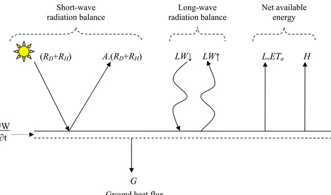
(4) Hobbins et al.. ∂W = R D + R H − A(R D + R H ) + LW ↓ − LW ↑ − Lv ETa − H − G ∂t. (1). where ∂W/∂t represents the time-change in heat storage of the evaporating layer, RD is the direct incident solar radiation, RH is the diffuse horizontal solar radiation, A is the global albedo, LW↓ is the long wave radiation from the atmosphere to the surface, LW↑ is the long-wave radiation in the opposite direction, the product LvETa is the latent heat flux, H is the sensible heat transfer from the surface to the atmosphere, and G is the ground heat flux. All negative or subtracted quantities are fluxes away from the surface.. Long-wave radiation balance. Short-wave radiation balance. (RD+RH). A.(RD+RH). LW↓. LW↑. Net available energy. LvETa. H. ∂W ∂t. G Ground heat flux. Figure 1: Schematic representation of the instantaneous energy budget at an evaporating surface.. In accumulating monthly evapotranspiration estimates over an integermultiple of years, G and ∂W/∂t are taken to be zero; that is, ground heat fluxes into the ground are balanced by fluxes out and there is no net change in heat storage in the evaporating layer. Thus, in making long-term estimates of ET, Eq. (1) devolves to Eq. (2):. Qn = Lv ETa + H = R D + RH − A(RD + RH ) + LW ↓ − LW ↑. 106. (2).
(5) Developing a Long-term, High-resolution, Continental-scale, Spatially Distributed Timeseries of Topographically Corrected Solar Radiation.. where the terms on the left—QN and (LvETa + H)—represent the energy available for evaporation. To calculate QN, both the short-wave and longwave radiation balances must be calculated (see Figure 1), and the radiative input to the short-wave balance corrected for topography. The short-wave balance is calculated as follows:. R N = (1 − A) * RG = (1 − A) * (RD + RH ). (3). where RN is net or absorbed global radiation, A is global albedo, and RG is incident global radiation, the sum of direct and diffuse incident radiation. The long-wave balance is calculated from:. B = LW ↑ − LW ↓ = σ T 4 (0.71 + 0.007 ea P 1013)(1 + ρ ) − σ T 4. (4). where B is the net long-wave radiation transfer to the evaporating surface, σ is the Stefan-Boltzmann constant, T is the air temperature, ea is the vapor pressure, P is the atmospheric pressure derived from elevation, and ρ is the proportional increase in atmospheric radiation due to clouds. The second term of Eq. (4) represents an empirical expression [Morton, 1978] for the incident long-wave radiation from atmosphere to ground. Eqs. (1) and (4) are then used to calculate QN corresponding to the soilplant surfaces at air temperature: Q N = R N + B − G = (1 − A) * (RD + R H ) + σ T 4 (0.71 + 0.007 ea P 1013)(1 + ρ ) − σ T 4 (5). Data Sources and Considerations:. Production of the time series of RN (see Eq. (3)) requires data on solar radiation (RD and RH), and global albedo (A). As shown in Eq. (5), then developing the QN time series further requires data on air temperature, humidity and pressure (T, ea, and P). The sources for these data are as follows: •. Solar Radiation: RD and RH data were extracted and temporally integrated on a monthly basis from three data sources representing sequential time periods: SOLMET [NCDC, 1978] for 1952-1960 (26 stations in the conterminous U.S.); “Solar and Meteorological Surface Observation Network (SAMSON)” [NOAA, 1993] for 1961-1990 (216 stations, of which 25% were 1st-order observing stations, and the rest of which were 2nd-order stations where solar data radiation were modeled); and “NCDC Surface Airways” [EarthInfo, 1998a] for 1991-1994 (25 stations). However, RH data were absent from both the SOLMET and the Surface Airways datasets and therefore had to be infilled, as outlined in the next 107.
(6) Hobbins et al.. section. The definitions of these two components of the short-wave radiation budget are as follows: o Direct Normal Solar Radiation, RD: This is defined as the amount of solar radiation received within a 5.7-degree field of view centered on the sun, and is measured by pyrheliometers. These instruments point directly at sun throughout its daily trajectory and measure the amount of solar radiation received within a 5.7-degree field of view, always centered on the sun. As this measurement technique is independent of local topography, corrections for slope and aspect of the surface are required for this quantity. o Diffuse Horizontal Radiation, RH. This is defined as the amount of solar radiation received from the sky (excluding the solar disk) on a horizontal surface, and is non-directional and therefore not significantly affected by local topography.. •. Albedo: Average monthly surfaces of A are AVHRR-derived estimates from the Gutman [1988] data set. This data set contains Advanced Very High Resolution Radiometer (AVHRR) derived albedo estimates, with an initial resolution of about 15 km.. •. Temperature: The T data were obtained from the “Summary of the Day” [EarthInfo, 1998b] CD-ROM, issued by NCDC.. •. Humidity: The ea data were obtained, initially in the form of dew-point temperature, from the “Surface Airways” [EarthInfo, 1998a] CD-ROM, issued by NCDC.. •. Elevation: These data were derived from a 30-arc-second DEM (NOAANGDC), and used to derive P for use in the derivation of QN, and converted to surfaces of slope and aspect for use in the topographic correction of RD.. Infilling the missing SOLMET and Surface Airways RH data:. In order to replicate the RH data missing from the SOLMET dataset for the years 1952-1960 and the RH data never recorded at the Surface Airways stations for the years 1991-1994, it was assumed that they bore significant physical relationships to the simultaneously recorded RD and RG data— neither of which were missing—and that the monthly relationships could be inferred using relationships between the RH, RD, and RG data recorded at the equivalent SAMSON stations during the years 1960-1990. Thus, for each of the 27 SOLMET and 25 Surface Airways stations, the corresponding SAMSON stations were identified, and their RH, RD, and RG data used in 108.
(7) Developing a Long-term, High-resolution, Continental-scale, Spatially Distributed Timeseries of Topographically Corrected Solar Radiation.. linear relationships to relate RH to RD alone, RG alone, and RD and RG together. The statistics of the regressed relationships were compared with respect to the coefficient of determination (R2) of the fit, its significance (pvalue), and the normality of the residuals as measured by a KolmogorovSmirnov test. Of the three possible relationships—RH ~ f(RD), RH ~ f(RG), and RH ~ f(RG,RD)—those with the highest R2 and p-values less than 0.05 were used. The R2 values for the RH ~ f(RG,RD) regression were in all cases the highest, ranging from 0.818 to 0.992, with an average value of 0.9512, and these relationships were applied to the SOLMET and Surface Airways RD and RG data to re-create the missing RH data for the years 1952-1960 and 1991-1994.. Solar Radiation Geometry:. It is important to note that the 2-dimensional surface of solar radiation shown in Figure 1 represents estimates of solar radiation on a level surface, i.e., a surface with no slope or aspect. The slope of a surface is its steepest slope in the vertical plane, subject to 0 < σ < π/2, and its aspect is the clockwise angle between the northward direction and the direction of the steepest slope projected onto the horizontal plane. In rugged terrain, therefore, the angle of incident radiation is altered, and greatly influences the amount of solar radiation incident on the surface by changing the effective area that a given packet of incoming solar radiation covers. Therefore, the interpolated value at each grid-cell must be adjusted to take into account its slope and aspect. To do this, RG—usually defined as the sum of RH and RD on a horizontal surface—must be separated into the two components and a topographic correction factor that is a function of the slope and aspect applied to RD, as shown in Eq. (6): RG = RH + R D . f (slope, aspect ). (6). In correcting the short-wave radiation balance for the effects of variable topography, we first seek to define the angle between the normal vector to an arbitrarily oriented ground surface and the vector parallel to the line of sight to the sun, as shown in Figure 2. In Figure 2, the definitions of the angles are as follows: µ on the x-y plane (N-W) is the azimuth angle, that is, the clockwise angle between the northward direction and the direction of the line of sight to the sun projected onto the horizontal plane; α on the x-y plane (N-W) is the aspect angle; σ on plane 0-b-d is the slope angle; Z on plane 0-S-b is the solar zenith angle, that is, the angle between the normal to a horizontal surface on the surface of the planet and the line of sight to the sun; and θ on plane S-0-G is the incidence angle, that is, the angle between the line of sight to the sun and the normal. 109.
(8) Hobbins et al.. vector to the arbitrarily oriented surface. This last is the angle we are interested in obtaining. where the numerator is the inner (or dot) product of the vectors A and B, and |A| and |A| and |B| are the magnitude (length) of vectors A and B, respectively. The inner product of any two n-dimensional vectors is defined as: cos Θ =. A•B AB. (7). From analytical geometry, the angle between any two vectors A and B is given by: n. A • B = ( a1 , a 2 ,..., a n ) • ( b1 ,b2 ,...,bn ) = ∑ ai bi. (8). i =1. and the magnitude as: G. b S. Z µ. σ c. 0 360 - α. West. d. a. North Figure 2: Direct solar radiation incident on an arbitrarily inclined surface (abc).. A = A•A =. n. ∑a i =1. 2 i. (9). 110.
(9) Developing a Long-term, High-resolution, Continental-scale, Spatially Distributed Timeseries of Topographically Corrected Solar Radiation.. In order to determine θ, then, we need to determine the unit vectors defining the directions of the gradient vector (steepest slope) and the line of sight to the sun. Let G be the gradient vector. Then, from simple geometry (see Figure 2) this vector is equal to: G = G (i sin σ cosα + j sin σ sin α + k cos σ ). (10). Let S be the vector parallel to the line of sight to the sun. Then, again from simple geometry (Figure 2) this vector is equal to: S = S (i sin Z cos µ + j sin Z sin µ + k cos Z ). (11). Finally, using (10) and (11) in (7): cos θ =. S•G SG. (12). and applying the definitions of inner product and magnitude, we obtain: [ S (i sin Z cos β + j sin Z sin β + k cos Z )] * cosθ =. [ G (i sin σ cos α + j sin σ sin α + k cos σ )]. (13). SG. Eq. (13) can be simplified to yield:. cosθ = sin Z cos β sin σ cosα + sin Z sin β sin σ sin α + cos Z cos σ. (14). Eq. (14) then defines the incidence angle θ between the vector gradient of any arbitrarily oriented surface and the line of sight to the sun. The cosine of this angle cosθ is then the correction factor to be applied to the magnitude of the direct solar radiation to resolve the effects of the topography of the evaporating surface. More conveniently (i.e., obviating calculations of solar zenith angle Z and solar azimuth angle β) [Iqbal, 1983], cosθ may be calculated from Eq. (15): cos θ = (sin φ cos β − cos φ sin β cos α )sin δ + (cos φ cos β + sin φ sin β cos α ) cos δ cos ω + cos δ sin β sin α sin ϖ (15) where δ is the solar declination (north positive), ω is the hour angle (0° at noon and morning positive), and φ is the latitude (north positive). Input surfaces of slope β and aspect α were derived from a DEM, and a surface of latitude φ was generated in the geographical projection domain.. 111.
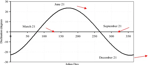
(10) Hobbins et al.. 30. June 21. Declination (degrees. 20 10. September 21. March 21 0. 0. 50. 100. 150. 200. 250. 300. 350. -10. -20. December 21 -30. Julian Day. Figure 3: Annual cycle of declination of the sun. Origin for time axis is January 1; north is positive.. The cycle of declination δ throughout the year (Figure 3) is calculated (in degrees) from:. δ=. 180 ⎛ 0.006918 − 0.39912 cos Γ + 0.0757 sin Γ − 0.006758 cos 2Γ ⎞ ⎜ ⎟⎟ π ⎜⎝ + 0.000907 sin 2Γ − 0.002697 cos 3Γ + 0.00148 sin 3Γ ⎠. (16). where Γ is the day angle (in radians), calculated from. Γ = 2π. JD − 1 365. (17). where JD is the Julian Day (January 1 = 1). The hour angle ω (in degrees) is 0˚ at noon, +15˚/hour between sunrise and noon, -15˚/hour between sunrise and sunset. The sunrise angles for flat surfaces are calculated from:. ϖ s = cos −1 (− tan φ tan δ ). (18). with the sunset angles given by -ωs. For a surface oriented toward the east (i.e., 0 < α < 180), the sunrise angle ωsr and sunset angle ωss are:. ⎡. ⎛ − xy − x 2 − y 2 + 1 ⎞⎤ ⎟⎥ 2 ⎜ ⎟⎥ x +1 ⎝ ⎠⎦. ϖ sr = min ⎢ϖ s , cos −1 ⎜ ⎢ ⎣. 112. (19a).
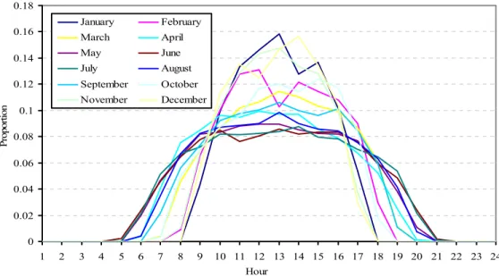
(11) Developing a Long-term, High-resolution, Continental-scale, Spatially Distributed Timeseries of Topographically Corrected Solar Radiation.. ⎡. ⎛ − xy + x 2 − y 2 + 1 ⎞⎤ ⎟⎥ 2 ⎜ ⎟⎥ + x 1 ⎝ ⎠⎦. ϖ ss = − min ⎢ϖ s , cos −1 ⎜ ⎢⎣. (19b). while for a surface oriented toward the west (i.e., 180 < α < 360), they are: ⎡. ⎛ − xy + x 2 − y 2 + 1 ⎞⎤ ⎟⎥ 2 ⎜ ⎟⎥ + x 1 ⎝ ⎠⎦. ϖ sr = min ⎢ϖ s , cos −1 ⎜ ⎢⎣. ⎡. ⎛ − xy − x 2 − y 2 + 1 ⎞⎤ ⎟⎥ 2 ⎜ ⎟⎥ + x 1 ⎝ ⎠⎦. ϖ ss = − min ⎢ϖ s , cos −1 ⎜ ⎢⎣. (19c). (19d). where: x=. cos φ sin φ , + sin α tan β tan α. ⎛ sin φ cos φ ⎞ ⎟⎟ . y = tan δ ⎜⎜ − ⎝ sin α tan β tan α ⎠. (20). From the equations above it is possible to derive the topographic correction factor cosθ for the incidence of direct solar radiation on arbitrarily oriented surfaces at any latitude at any moment in any day of the year. However, this correction factor is not constant, as the position of the sun in the sky (vector S) varies with season and time of day. In running the models at a monthly time-step, it is necessary to correct monthly radiation totals for use in Eq. (6). Therefore, we must derive monthly magnitude-weighted correction factors that account for the intra-monthly periodicity in cosθ. Incidence angles θi were generated for each daylight hour of the 15th of each month at each grid-cell in the conterminous US. The 15th day was assumed to represent the mean astronomical parameters for the month, with 10 years of data used to generate a mean 15th day. The monthly values of cosθ were then derived as a weighted average of the hourly proportion values pi for the 15th day of each month as shown in Eq. (21): 21. cosθ MONTH = ∑ cosθ i . pi. (21). i =5. where cosθMONTH is the monthly topographic correction factor for direct solar radiation, the index i represents the daylight hours from 5 to 21, Si is the direct solar radiation for hour i, and pi is the proportion of the daily total of direct solar radiation received in hour i, on day 15 of each month, based on a 10-year average of 15th days. The variation of pi is shown for a single example station in Figure 4. The derivation of the pi surfaces is described below.. 113.
(12) Hobbins et al.. 0.18 0.16 0.14. Proportion. 0.12. January. February. March. April. May. June. July. August. September. October. November. December. 0.1 0.08 0.06 0.04 0.02 0 1. 2. 3. 4. 5. 6. 7. 8. 9. 10 11 12 13 14 15 16 17 18 19 20 21 22 23 24 Hour. Figure 4: Hourly proportions of direct solar radiation for the 10-year average 15th day of each month at Fargo, ND.. Hourly proportions of direct solar radiation pi values were calculated for each station as the mean of 10 years of hourly data for day 15 of each month. For the lower-48 states, i ranges from 5 to 21. Station values of pi were regressed against latitude to create trend surfaces, in order to generate trend surfaces to improve their spatial interpolation. The station values for hourly totals of direct solar radiation Si in the 15th day were regressed on station latitude, longitude and elevation, taken singly and in all combinations. Then, for each month, the hourly pi surfaces from the initial interpolation run were corrected using Eq. (22): pi =. Si. ⇒. 21. ∑S i =5. 21. ∑p i =5. i. = 1.. (22). i. in order that any negative values introduced by the spatial interpolation algorithm were eliminated, and that hourly proportions pi for each cell summed to one.. 114.
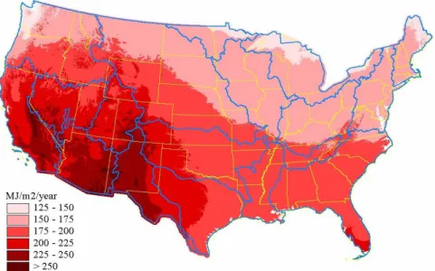
(13) Developing a Long-term, High-resolution, Continental-scale, Spatially Distributed Timeseries of Topographically Corrected Solar Radiation.. 3. Results. In this section we present some preliminary results of our development of the dataset: namely 5-km resolution surfaces of the mean annual QN and the trends in annual RG. It should be re-emphasized that these results are only preliminary, as the errors that may have been introduced to the dataset due the spatial interpolation procedures in any of the station-based inputs, or to heterogeneities incurred in the marriage of the datasets, which individually may be assumed to be homogenous need to be checked. Nonetheless, broad conclusions may still be drawn from these results. Figure 5 presents the mean annual surface of QN over the conterminous U.S. at a 5-km resolution for the period WY 1953-1994. QN is that portion of the surface energy budget that is available for the evaporative process. Obvious in this figure is the effect of insolation’s inverse latitudinal trend, particularly over the homogenous eastern U.S.. In the western U.S., where the effects of topography on the direct normal radiation RD component of QN are more pronounced, the pattern of insolation is evidently more attuned to elevation, or more specifically, to the increased slopes and more varied aspects that accompany rugged terrain.. Figure 5: Distributed mean annual QN, spatially interpolated across the conterminous U.S. from a 42-year (WY 1953-1994) monthly time-series of observations, expressed as the arithmetic mean of the time-series of annual totals at each pixel, in MJ/m2/year. Also shown are the state and water resource region boundaries.. 115.
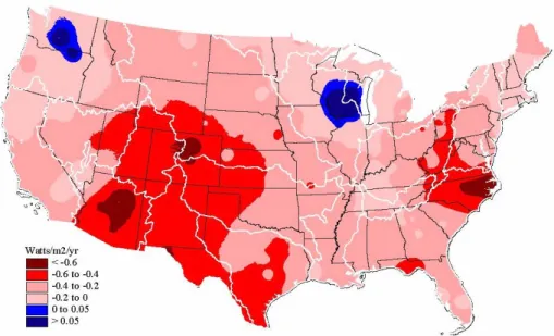
(14) Hobbins et al.. Figure 6: Distributed trends in mean annual incident solar radiation RG spatially interpolated across the conterminous U.S. from a 42-year (WY 1953-1994) monthly time-series of observations, corrected for local topographic effects, and expressed as the slope of a linear fit to the annual time series at each pixel, in watts/m2/year. Also shown are the state and water resource region (WRR) boundaries.. Figure 6 presents the temporal trend in incident solar radiation RG, expressed as the slope of a linear fit to a 42-year annual time-series. RG is the sum of RH and topographically adjusted RD (see Eq. (6)), and provides the major energy input to any evaporative process, and when applied to a surface energy budget, (see Eq. (5)) is an excellent estimator of QN, which is then the energy available at the surface for evaporation (see Figure 5). The existence of trends in RG appears in the literature to be somewhat of a hot-button issue: predictions by GCMs are not matched by observations of decreasing shortwave irradiance at the earth’s surface on the order of over 10% over the past 50 years [Gilgen et al., 1998], an observed decrease in global solar irradiance of 6-12% over the period 1960-1990 for a region in northwestern Russia [Roderick and Farquhar, 2002], or of globally increasing cloudiness and precipitation [Karl et al., 1996]. We have no data for Russia but, averaged across the conterminous U.S. for the period of our dataset (WY 1953-1994), we observe a decrease in RG of 0.298 watts/m2/year, for a 42year decrease of 12.52 watts/m2 or 14.4% of the mean, thereby lending indirect support to the findings of and Gilgen et al. [1998]. On a distributed basis, the pattern of decreasing RG is almost universal—with RG decreasing over 97.50% of the conterminous U.S., with decreases pronounced in the Southwest and North Carolina. Significant exceptions to this general decrease are evident in the western Great Lakes region and the inland Pacific Northwest. 116.
(15) Developing a Long-term, High-resolution, Continental-scale, Spatially Distributed Timeseries of Topographically Corrected Solar Radiation.. 4. Conclusions Towards the development of an accurate distributed dataset of ETa based on the complementary relationship as a tool for studies of climate change and variability across the conterminous U.S., the authors created a 42-year-long set of monthly, spatially distributed, high-resolution surfaces of QN that accounts for the effects of topography on RD. This involved the collation of RD and RH data from three sources, the reproduction of 12 years of monthly RH radiation data missing from two of the sources, and the development of an algorithm for topographic corrections of RD at a point. The spatial resolution of the resulting QN dataset is determined only by the resolution of the DEM used to derive the slope and aspect surfaces. The temporal resolution was matched to that of the other input data to the ETa model and, while it is theoretically variable, it is practically fixed by dint of the computational investment of the input surfaces to the solar radiation adjustment procedure described. This new QN dataset allows for long-term trend analyses in the single most important variable in determining the strength of the hydrologic cycle to be studied, as shown in Hobbins et al. [2001c], where δQN was analyzed as a component of δETa, allowing for falsification of other earlier work concerning the trends in ETa and pan evaporation [Szilagyi et al., 2001; Roderick and Farquhar, 2002]. Further, the spatial distribution of the dataset allows for analysis of un-metered regions, but at a cost of generating uncertainties associated with spatial interpolation of the input data. It allows the further breakdown of climatic trends in the components of the hydrologic cycle, particularly those components of ETa, as to both their magnitude and their spatial distribution. Such data are available for anywhere in the conterminous U.S. and at any scale and spatial breakdown so desired: from the entire conterminous U.S.; into water resource regions, states, climatic divisions, specific watersheds, physiographic regions; and on down to that of a single pixel. This represents a significant leap forward from previous studies, both in that our spatially distributed technique allows us to examine regional sensitivities to climate change and variability—a significant improvement over generating continental-scale averages from point values— and in that examining long-term trends in the input climatic variables allows us to avoid making any assumptions of stationarity in any component, specifically QN. Further work will include an examination of the homogeneity of the input data, especially at temporal joints, the solar-shadowing effects of regional topography, and an estimation of the accuracy of the technique using the missing station interpolation test and others.. 117.
(16) Hobbins et al.. 5. References Bouchet, R. J., 1963: Évapotranspiration réelle et potentielle, signification climatique. Int. Assoc. Sci. Hydrology, Proc. Berkeley, California, U.S.A., Symp., Publ. No. 62: 134– 142. Brutsaert, W., and H. Stricker, 1979: An advection-aridity approach to estimate actual regional evapotranspiration. Water Resources Research, 15(2): 443–450. Chiew, F. H. S., and T. A. McMahon, 1996: Trends in historical streamflow records. Regional Hydrological Response to Climate Change, J. A. A. Jones et al., Ed., Kluwer Academic Publishers, Amsterdam: 63–68. Claessens, L., J. A. Ramírez, and T. C. Brown, 1995: Estimation of areal evapotranspiration: evaluation of the complementary relationship using long-term large-scale water budgets. Proceedings of the Fifteenth Annual American Geophysical Union Hydrology Days. Colorado State University, Fort Collins, Colorado, U.S.A.: 1–16. EarthInfo, 1998a: NCDC Surface Airways [TD-3280 computer file]. Boulder, Colorado, U.S.A. EarthInfo, 1998b: NCDC Summary of the Day [TD-3200 computer file]. Boulder, Colorado, U.S.A. Eitzinger et al., personal communication, 2001 Gilgen, H., M. Wild, and A. Ohmura, 1998: Means and trends of shortwave irradiance at the surface estimated by from Global Energy Balance Archive data, Journal of Climate, 11: 2042–2061. Gutman, G., 1988: A simple method for estimating monthly mean albedo from AVHRR data. Journal of Applied Meteorology, 27(9): 973–988. Hobbins, M. T., J. A. Ramírez, T. C. Brown, and L. H. J. M. Claessens, 2001a: The complementary relationship in estimation of regional evapotranspiration: the CRAE and Advection-aridity models. Water Resources Research, 37(5): 1367–1388. Hobbins, M. T., J. A. Ramírez, and T. C. Brown, 2001b: The complementary relationship in estimation of regional evapotranspiration: an enhanced Advection-aridity model. Water Resources Research, 37(5): 1389–1404. Hobbins, M. T., J. A. Ramírez, and T. C. Brown, 2001c: Trends in regional evapotranspiration across the United States under the complementary relationship hypothesis. Proceedings of the Twenty-first Annual American Geophysical Union Hydrology Days. Colorado State University, Fort Collins, Colorado, U.S.A.: 106–121. Iqbal, M., 1983: An Introduction to Solar Radiation. Academic Press, New York, NY, USA. 390 pp. Karl, T. R., and R. W. Knight, 1998: Secular trends of precipitation amount, frequency, and intensity in the United States. Bulletin of the American Meteorological Society, 79(2): 231–241. Karl, T. R., R. W. Knight, D. R. Easterling, and R. G. Quayle, 1996: Indices of climate change for the United States. Bulletin of the American Meteorological Society, 77(2): 279–292. Lettenmaier, D. P., E. F. Wood, and J. R. Wallis, 1994: Hydro-climatological trends in the continental United States, 1948–88. Journal of Climate, 7: 586–607. Lins, H. F., 1997: Regional streamflow regimes and hydroclimatology of the United States. Water Resources Research, 33(2): 1655–1667. Lins, H. F. and J. R. Slack, 1999: Streamflow trends in the United States. Geophysical Research Letters, 26(2): 227–230. Lockwood, J. G., 1994: Climatic change, grass pasture and potential evapotranspiration. Weather, 49(9): 318–321. Morton, F. I., 1978: Estimating evapotranspiration from potential evaporation: practicality of an iconoclastic approach, Journal of Hydrology, 38: 1–32. Morton, F. I., 1983: Operational estimates of areal evapotranspiration and their significance to the science and practice of hydrology. Journal of Hydrology, 66: 1–76.. 118.
(17) Developing a Long-term, High-resolution, Continental-scale, Spatially Distributed Timeseries of Topographically Corrected Solar Radiation. National Climatic Data Center (NCDC), 1978: SOLMET, User’s Manual – Hourly Solar Radiation – Surface Meteorological Observations, Vol. 1, National Climatic Data Center, Asheville, NC. National Oceanic and Atmospheric Administration (NOAA), 1993: Solar and Meteorological Surface Observation Network 1961-1990 (CD-ROM), Version 1.0. National Climatic Data Center, EDIS, Federal Building, Asheville, NC. Szilagyi, J., G. G. Katul, and M. B. Parlange, 2001: Evapotranspiration Intensifies over the Conterminous United States. Journal of Water Resources Planning and Management, 127(6), 354–362. Szilagyi, J., 2001: Modeled Areal Evaporation Trends over the Conterminous United States. Journal of Irrigation Drainage and Engineering, July/August, 196–200. Roderick, M.L. and G.D. Farquhar, 2002: The cause of decreased pan evaporation over the past 50 years. Science, 298, 1410–1411. Wahl, K. L., 1992: Evaluation of trends in runoff in the western United States. Proceedings, Managing Water Resources During Global Change, 28th Annual Conference and Symposium, Reno, NV, American Water Resources Association, 701–710. Westmacott, J. R., and D. H. Burn, 1997: Climate change effects on the hydrologic regime within the Churchill-Nelson River Basin. Journal of Hydrology, 202: 263–279.. 119.
(18)
Figure

+3
Related documents
The Dosepix frontend can be described with the so-called paralysable detector model with respect to pulse pileup [2], which means that there can be an accumulation of multiple
a The capillary flow of a sample liquid in a constant cross-section capillary depends on the sample liquid properties; b adding a second liquid, the pump liquid generates a
It is also shown that a lower shielding thickness when encountering SPEs, for example when in a space suit, is useful as long as the total amount of time spent in this suit during
Table 4.12: Data showing the difference between insulated and non-insulated construction with outdoor temperature -10 ºC and concrete top layer in dry model calculations...
Morris, Mechanical instability and ideal shear strength of transition metal carbides and nitrides, Phys. Ihm, Vacancy hardening and softening in transi- tion metal carbides
Teorin om neopatrimonialism kommer för denna studie att vara underordnad de andra och enbart tillämpas till denna forskning i syfte att komplettera tänkbara tillkortakommanden som
Zwei Schwerterzeigten Spuren von Nickel, eine Speerspitze 0,17 °/o, eine Pfeilspitze 0,6 °/o, die iibrigen Gegenstände (Messer, Axt, Nagel u n d Nieten) weniger als 0,1
It is shown that as the duration of the excitation current of the dipole decreases with respect to the travel time of the current along the dipole, P → U/c where P is the net
