Supervisor: Alireza Malehmir
Examensarbete vid Institutionen för geovetenskaper
ISSN 1650-6553 Nr 266
Analysis and Interpretation of 2D/3D
Seismic Data over Dhurnal Oil Field
Northern Pakistan
i
Abstract
The study area, Dhurnal oil field, is located 74 km southwest of Islamabad in the Potwar basin of Pakistan. Discovered in March 1984, the field was developed with four producing wells and three water injection wells. Three main limestone reservoirs of Eocene and Paleocene ages are present in this field. These limestone reservoirs are tectonically fractured and all the production is derived from these fractures. The overlying claystone formation of Miocene age provides vertical and lateral seal to the Paleocene and Permian carbonates. The field started production in
May 1984, reaching a maximum rate of 19370 BOPD in November 1989. Currently Dhurnal‐1
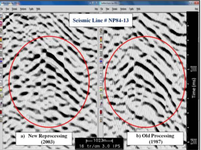
(D-1) and Dhurnal‐6 (D-6) wells are producing 135 BOPD and 0.65 MMCF/D gas. The field has depleted after producing over 50 million Bbls of oil and 130 BCF of gas from naturally fractured low energy shelf carbonates of the Eocene, Paleocene and Permian reservoirs. Preliminary geological and geophysical data evaluation of Dhurnal field revealed the presence of an up-dip anticlinal structure between D-1 and D-6 wells, seen on new 2003 reprocessed data. However, this structural impression is not observed on old 1987 processed data. The aim of this research is to compare and evaluate old and new reprocessed data in order to identify possible factors affecting the structural configuration. For this purpose, a detailed interpretation of old and new reprocessed data is carried out and results clearly demonstrate that structural compartmentalization exists in Dhurnal field (based on 2003 data). Therefore, to further analyse the available data sets, processing sequences pertaining to both vintages have been examined. After great effort and detailed investigation, it is concluded that the major parameter giving rise to this data discrepancy is the velocity analysis done with different gridding intervals. The detailed and dense velocity analysis carried out on the data in 2003 was able to image the subtle anticlinal feature, which was missed on the 1987 processed seismic data due to sparse gridding. In addition to this, about 105 sq.km 3D seismic data recently (2009) acquired by Ocean Pakistan Limited (OPL) is also interpreted in this project to gain greater confidence on the results. The 3D geophysical interpretation confirmed the findings and aided in accurately mapping the remaining hydrocarbon potential of Dhurnal field.
ii
Acknowledgements
Alhamdulillah, all praise to Allah (Subhana wa ta’alaah) for his graciousness and mercy upon me. I am sincerely thankful to my supervisor, Dr. Alireza Malehmir, for his prompt and valuable guidance and encouragement extended to me.
Most importantly, I am grateful to Mr. Zaheer A. Zafar, Manager Geophysics, Ocean Pakistan Limited, for his technical support and guidance throughout my research work. Moreover, all 2D and 3D geological and geophysical data used in my research are owned and kindly provided by Ocean Pakistan Limited.
I am also deeply thankful to all my loved ones, including my family and friends, especially my brother Humza, and my friend, Darina Buhcheva, for their unconditional love and support throughout my studies in Sweden. Lastly, I cannot imagine my academic journey in Sweden without my husband, Umair. Thank you for believing in me and motivating me to turn my dreams into reality.
iii
DEDICATION
To my beloved parents and husband, who have always been by my side …
v Table of contents Abstract……….……….……...…………...…. Acknowledgements………..……….………..………. List of Figures………...…... List of Abbreviations………..………...….. Chapter 1……….…………..……….. 1.1 Introduction……….………. 1.2 Study area……….………... 1.3 Stratigraphy of the area………..………..….………….. 1.3.1 Geological and geophysical data……….………..……... 1.3.2 2D Seismic data……….………….. 1.3.3 Well data……….………..….….. 1.3.4 3D Seismic data……….……..…… 1.3.5 Software used……….………..….…..………. 1.4 Problem identification………….……….…...….………… 1.5 Objectives………..…..…...
Chapter 2 2D Geophysical Evaluation…………..………...…….….
2.1 2D Seismic interpretation………...…. 2.1.1 Comparison of results of 2D interpretation based on 1987 and 2003 proc. data….. 2.2 Seismic data processing/reprocessing………..…. 2.2.1 Comparison of two processing sequences ………..………… 2.3 Velocity analysis ……….…... 2.3.1 Comparison of results of velocity analysis based on 1987 & 2003 data…...
Chapter 3 3D Seismic Geophysical Evaluation ………...
3.1 3D seismic data interpretation………..…. 3.2 Results of 3D geophysical analysis………..…………..……
Chapter 4………... 4.1 Discussion ……….………..………... 4.2 Conclusions……….………. References………...………..……..……….. i ii vi ix 1 1 4 5 8 8 8 8 8 9 10 12 12 20 20 21 21 25 28 28 32 33 33 34 35
vi
List of Figures
Figure 1.1: Map showing sedimentary basins of Pakistan and location of the study area; marked
by green region (modified after Ahmed et al., 1994)………..………
Figure 1.2: Exploration (oil/gas) wells location map of Potwar basin and part of Kohat
sub-basin (Source: DGPC; Redrawn)………..……….…..……
Figure 1.3: Location map of the Dhurnal oil field (Source: PPIS) which is the area of interest in
this study ……….…………...……….
Figure 1.4: Coordinate map of the Dhurnal oil field (Source: Ocean Pakistan Limited). Dhurnal
oil field is the focus of this thesis. Green dots indicate the locations of four producing wells (D-1, D-2, D-3 and D-6) and the rest of the dots show the locations of water injection wells (D-4, D-5 and D-7)………..……….
Figure 1.5: Generalized stratigraphic column of the Dhurnal field (Source: Ocean Pakistan
Limited). Eocene and Paleocene are the main reservoirs in Dhurnal area and main target horizons of 2D/3D seismic data interpretation in this thesis………...….
Figure 1.6: Comparison of a) new 2003 reprocessed and b) old 1987 processed seismic data on
seismic line number NP84-13, generated using SeisWorks® 2D workstation. The zone of interest is marked with red circles on both seismic sections..….………..…..
Figure 2.1: Vertical seismic profile (VSP) of Dhurnal-1 well used for horizon identification. The
vertical panels above show the different processing levels. The red circle indicates the Eocene level which is the main reservoir in the Dhurnal field (Source: OPL)……..……….…..….
Figure 2.2: Horizon interpretation on seismic line NP84-13 (1987 data). Yellow color shows
Eocene reflector and the rest of colors indicates fault interpretation. ……….…………
Figure 2.3: Horizon interpretation on seismic line NP84-13 (2003 data). Yellow color shows
Eocene reflector and the rest of colors indicates fault interpretation……….…………..
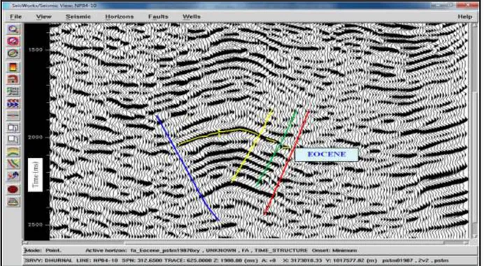
Figure 2.4: Horizon interpretation on seismic line NP84-10 (1987 data). Yellow color shows
Eocene reflector and the rest of colors indicate fault interpretation. …...
Figure 2.5: Horizon interpretation on strike line NP84-52 (2003 data). The Eocene reflector is
marked and fault interpretation is also visible in this section. The inset map shows the location of this line highlighted by red……….
2 3 4 5 7 10 13 14 15 16 16
vii
Figure 2.6: Composite line passing through D-3 and D-6 wells (1987 data). This display clearly
indicates downthrown block at the reservoir level on line NP84-13. Eocene level is displayed by yellow color. The inset map shows the location of these line highlighted by red……….17
Figure 2.7: Composite line passing through D-3 and D-6 wells (2003 data). This display clearly
indicates the presence of anticlinal feature at reservoir level on line NP84-13. Eocene level is displayed by yellow color. The inset map shows the location of these lines highlighted by
red………...
Figure 2.8: Time structure map at Top Eocene level based on 1987 reprocessed PSTM data. The
black-colored time contours show that a downthrown block exists between D-1 and D-6 wells. The fault polygons are represented as grey where the fault arrows indicate a thrust regime and purple lines are the Dhurnal mining lease………...……...
Figure 2.9: Time structure map at Top Eocene level based on 2003 reprocessed PSTM data.
According to black-colored time contour values, a pop-up anticlinal structure separates D-1 and D-6 wells. The fault polygons are represented as grey where the fault arrows indicate a thrust regime and purple lines are the Dhurnal mining lease……….……...…...
Figure 2.10: Comparison of old 1987 and new 2003 processing/reprocessing of PSTM data
showing the presence of pop-up anticline in 2003 data. However, a downthrown block is observed exactly at the same shot point location on 1987 data……….………....
Figure 2.11: Sparse velocity picking on old 1987 data showing vertical velocity panels at the top
of the seismic section. In this case, the velocity grid is 1 km apart displaying the zone of interest as a downthrown block between D-1 and D-6 wells………..………..……..
Figure 2.12: Detailed velocity picking on 2003 data showing vertical velocity panels at the top
of the seismic section. In this case, the velocity grid is 0.5 km apart displaying a pop-up anticlinal structure (an up-thrust block) between D-1 and D-6 wells………..…….………
Figure 2.13: Velocity map based on 1987 data showing a velocity anomaly in the south of D-1
and D-6 wells. Black contours represent velocity trend (meter/second) in the area and purple lines are the Dhurnal mining lease………...
Figure 2.14: Velocity map based on 2003 data showing a velocity anomaly over the apex of
Dhurnal structure. Black contours represent velocity trend (meter/second) in the area and purple lines are the Dhurnal mining lease………...
18 19 19 21 22 23 24 25
viii
Figure 2.15: Depth map based on 1987 data showing lack of presence of any structural high
between D-1 and D-6 wells. The depth contours are drawn in black, fault polygons are
represented as grey and purple lines are the Dhurnal mining lease…..……….………..….
Figure 2.16: Depth map based on 2003 data showing the presence of a structural high between
D-1 and D-6 wells. The depth contours are drawn in black, fault polygons are represented as grey and purple lines are the Dhurnal mining lease………...…...…………
Figure 3.1: Characteristics of extracted wavelet (generated using SynTool™ software). The
figure shows that the dominant frequency of the actual seismic data at Eocene level is 15Hz……...
Figure 3.2: Geo-seismic calibration showing the synthetic seismogram displayed over the real
seismic section to identify Eocene reflector. A reasonable well to seismic tie can be observed in the figure……….……
Figure 3.3: Time map at Top Eocene level based on 3D data confirms the existence of structural
high between D-1 and D-6 wells. The aerial closure of this anticline is 143 acres (dark green polygon) whereas the total area of Dhurnal structure comes out to be 3422 acres.……….
Figure 3.4: Depth map at Top Eocene level based on 3D data showing up-dip area between the
D-1 and D-6 wells. The color bar shows yellow as shallowest and blue as deepest. The depth contours are drawn in black, fault polygons are represented as grey and purple lines are the Dhurnal mining lease………..………...…………
26 27 29 30 31 32
ix
List of Abbreviations
BCF Billion Cubic Feet Bbls Barrels
BOPD Barrels of Oil per day CDP Common Depth Point D-1 Dhurnal-1 well
D-6 Dhurnal-6 well
DGPC Directorate General Petroleum Concession of Pakistan FSI, UK Fugro Seismic Imaging Limited, United Kingdom Ft Feet
G & G Geological and Geophysical L.Km Line Kilometer
MMCF/D Million Cubic Feet per Day Ms Millisecond
OXY Occidental Pakistan Inc. OPL Ocean Pakistan Limited
OPI Orient Petroleum International
PGS Petroleum Geo-Services Data Processing, Cairo PPIS Pakistan petroleum information services
Proc. Processed
PSTM Pre-Stack Time Migration PSDM Pre-Stack Depth Migration RMS Vel. Root Mean Square Velocity TWT Two-way Travel Time VSP Vertical Seismic Profile
1
CHAPTER 1
1.1 Introduction
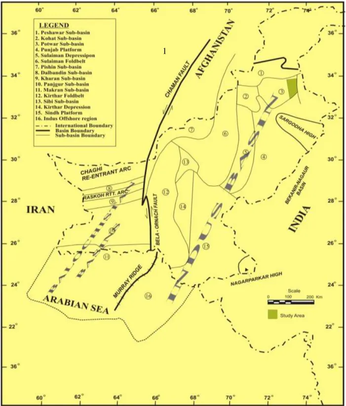
Pakistan hosts two major sedimentary basins namely, Indus and Balochistan having an area of around 83,000 sq.km involving both onshore and offshore (Kazmi HA and Jan QA, 1997). The Indus basin extends east-southeast into India and north-northeast into Afghanistan. The Balochistan basin lies west of Indus basin and continues northwards into Afghanistan and westwards into Iran. The two basins are separated by north-south trending left-lateral Bela-Ornach-Chaman transform fault zone and Murray ridge (Ahmed et al., 1994; Figure 1.1).
Pakistan represents the most spectacular collision and subduction region of the world (Raza et al., 1989). The Indus basin is located on Indian plate which collided with the Eurasian plate in the north during the Mid-Eocene time (Molnar and Tapponnier, 1975) while the Balochistan basin is formed between a remnant arc in the north and active subduction zone of Arabian plate beneath a block of Eurasian plate in the south (Raza et al., 1989). The geology of Pakistan has been extensively studied by many explorers and scientists, for example, Patriat and Achache, 1984; Pascoe, 1959; Powell, 1979 and Sclater and Fisher, 1974.
The Potwar basin is the part of Indus basin and is located at the northern rim of Indian plate in the foothills of western Himalayas in Pakistan (Iqbal and Ali, 2001 and Porth and Raza, 1990). The basin is the oldest and one of the major hydrocarbon producing regions of Pakistan.
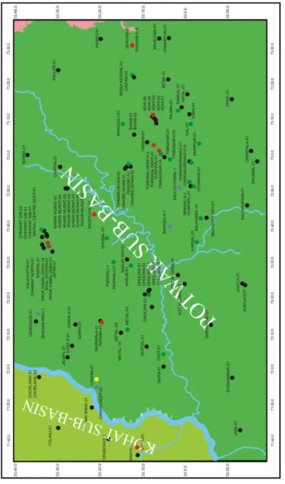
Figure 1.2 shows the number of exploration (oil/gas) wells drilled in this basin. These wells have an average depth ranging between 12000 – 14000 feet.
2
Figure 1.1: Map showing sedimentary basins of Pakistan and location of the study area; marked
by green region (modified after Ahmed et al., 1994). 1
3 Figu re 1 .2 : Explora tion ( oil /gas) w ell s loca ti on map of P otwa r sub -b asin a nd pa rt of Koha t s u b -b asi n (Sourc e: DGPC ; r edr awn) .
4
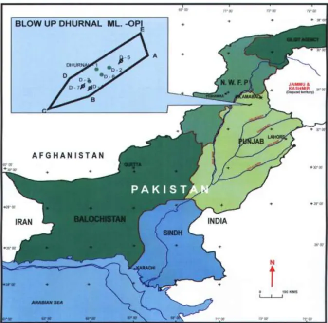
1.2 Study area
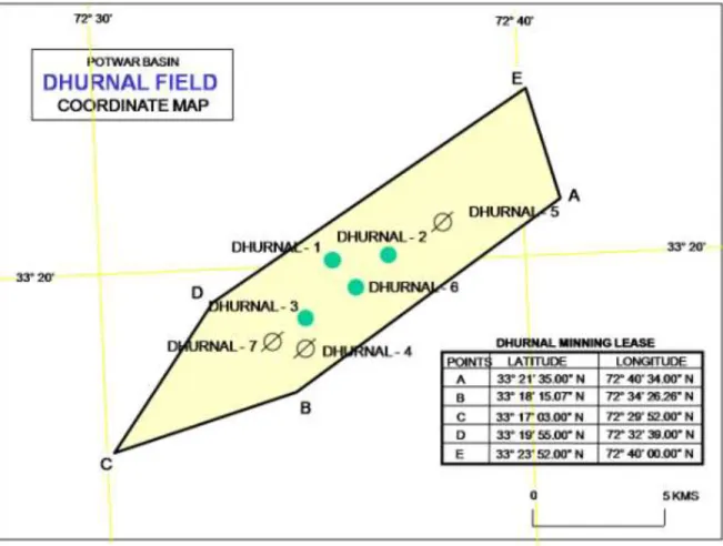
This research addresses the Dhurnal oil field, located in the central north part of the Potwar basin, in the northern region of Pakistan (Figure 1.3). The coordinate map of Dhurnal mining lease is shown in Figure 1.4.
Dhurnal structure is a typical Potwar pop‐up thrust bounded structure with four-way closure at the Eocene level in subsurface.
Figure 1.3: Location map of the Dhurnal oil field (Source: PPIS) which is the area of interest in
5
Figure 1.4: Coordinate map of the Dhurnal oil field (Source: Ocean Pakistan Limited). Dhurnal
oil field is the focus of this thesis. Green dots indicate the locations of four producing wells (D-1, D-2, D-3 and D-6) and the rest of the dots show the locations of water injection wells (D-4, D-5 and D-7).
1.3 Stratigraphy of the area
The general stratigraphy of the Dhurnal field is illustrated in Figure 1.5. Infra Cambrian Salt Range formation (evaporates) is the oldest drilled horizon, whose thickness is unknown. The formation is at least 287 ft (87.47 m) thick in Dhurnal-3.
The Permian rocks unconformably overlie Salt Range formation, and consist of about 2500 ft (762 m), of clastics and carbonates deposited in glacial, fluvial and shallow marine environments. There is a poorly defined angular unconformity between the Cambrian and the Permian rocks. Another major unconformity is present between the Late Permian and Paleocene formations.
6
In the early Paleocene time, a marine transgression resulted in early Tertiary sedimentation over the eroded older-strata. These shallow marine carbonates and coastal brackish water clastic attained their maximum thickness about 2500 ft (762 m) in the west of the basin, and thin depositionally to the east. In the Dhurnal field, the average thickness of the Paleogene section is about 1200 ft (365.74).
In the late Eocene time, early stages of the Himalayan orogenic movement uplifted the section, resulting in non-deposition throughout Oligocene time. The orogenic foredeep, trending northeast to southwest through Islamabad, was developed in Miocene. The foredeep was filled with molasses detritus up to 20,000 ft (6100 m) thick, derived from rapid erosion of the rising mountains in the north. Average thickness of the molasses in Dhurnal field is about 12500 ft (3810 m). The overlying claystone formation of Miocene age provides vertical and lateral seal to the Paleogene and Permian limestones. The stratigraphy of Potwar sub-basin has been studied by many geologists, such as Lillie et al., 1986; Pilgrim, 1913; Pinfold, 1918 and Davies LM and Pinfold E, 1937.
After the deposition of molasses, the basin suffered a severe orogenic phase in Pleistocene resulting in significant shortening of the stratigraphic section. This phase was associated with folding, faulting and uplift of all the elements in the basin. The structural relief of the Dhurnal field was developed at this time (about 3 million years ago).
7
Figure 1.5: Generalized stratigraphic column of the Dhurnal field (Source: Ocean Pakistan
Limited). Eocene and Paleocene are the main reservoirs in Dhurnal area and main target horizons of 2D/3D seismic data interpretation in this thesis.
8
1.4 Geological and geophysical data 1.4.1 2D seismic data
2D seismic data used in this study are:
1. AMOCO 1972 seismic data: total 105.924 L.km 2. OXY 1984 seismic data: total 245 L.km
3. OPI 2000 seismic data: total 16.6 L.km 4. Seismic data acquisition reports
5. Seismic data processing reports (PGS, 2003).
1.4.2 Well data
The following well data were available in the study area and used in this research work: 1. Total of 7 wells (D-1 to D-7) drilled in this area
2. VSP data 3. E-Logs
4. Well completion reports 5. Well summary sheets
1.4.3 3D seismic data
2D results were further verified by using 3D geophysical data, listed below: 1. 105 sq.km of 3D seismic data
2. Acquisition report
3. Processing report (Twyford I, 2010).
1.4.4 Software used:
LandMark suite of software developed by Halliburton were used for seismic data interpretation. The software and their specifications are listed as follows:
1. OpenWorks® R2003 2. OpenWorks® R5000
3. SeisWorks® 2D Seismic interpretation software 4. SuperSeis® 3D Seismic interpretation software
9 5. ZMap Plus™ Mapping and gridding software 6. SynTool™ Synthetic seismogram software
1.5 Problem identification
Critical review of the data revealed the development of a very strange structural feature on seismic line number NP84-13. The seismic processing carried out by Golden Geophysical in 1987, referred to as old processing in this research, indicated a downthrown block between Dhurnal-1 and Dhurnal-6 wells on line number NP84-13 (Figure 1.6b). However, the new reprocessing carried out on the same seismic line done by PGS in 2003 showed an up-thrust/pop-up structure at the same shot point position (Figure 1.6a). Moreover, it is interesting to note that both data sets had been processed using PSTM method.
This striking difference in the data may lead to some very important sub-surface structural features that were not identified earlier. The scope of this research was to carry out a complete and detailed analysis of the available data information in order to identify the principal factor creating this vital discrepancy in the two data sets.
10
Figure 1.6: Comparison of a) new 2003 reprocessed and b) old 1987 processed seismic data on
seismic line number NP84-13, generated using SeisWorks® 2D workstation. The zone of interest is marked with red circles on both seismic sections.
1.6 Objectives
The main objectives of this research are listed below:
1. To compare and evaluate old and new reprocessed data in order to identify possible factors affecting the structural configuration (Figure 1.6).
2. Interpret 2D seismic data and see the results in a planar view by generating time structure maps on the two data sets.
3. Detailed analysis of the processing/reprocessing sequences pertaining to old (1987) and new (2003) 2D seismic data.
4. Well seismic correlation by generating synthetic seismogram.
11
6. Construct and generate time and depth maps at target reservoir horizon (Top Eocene level) using LandMark SeisWorks® software.
7. Results may indicate that sharp velocity analysis done on 2003 data enabled in delineating subtle sub-surface features which were not identified earlier due to coarse velocity analysis carried out on 1987 data.
12
CHAPTER 2
2D geophysical evaluation
To verify that the up-dip structuring in the sub-surface observed on 2003 reprocessed data exists only on one line or extends through the area, two separate interpretation exercises were carried out, and time contour, velocity and depth maps were generated at reservoir horizon (Top Eocene level).
The detailed procedure of the geophysical work is explained below:
2.1 2D geophysical interpretation
Seismic interpretation was carried out on PreSTM time volume of 2D seismic data. SeisWorks® 2D seismic interpretation software application of LandMark suite of softwares developed by Halliburton was used for data interpretation purposes.
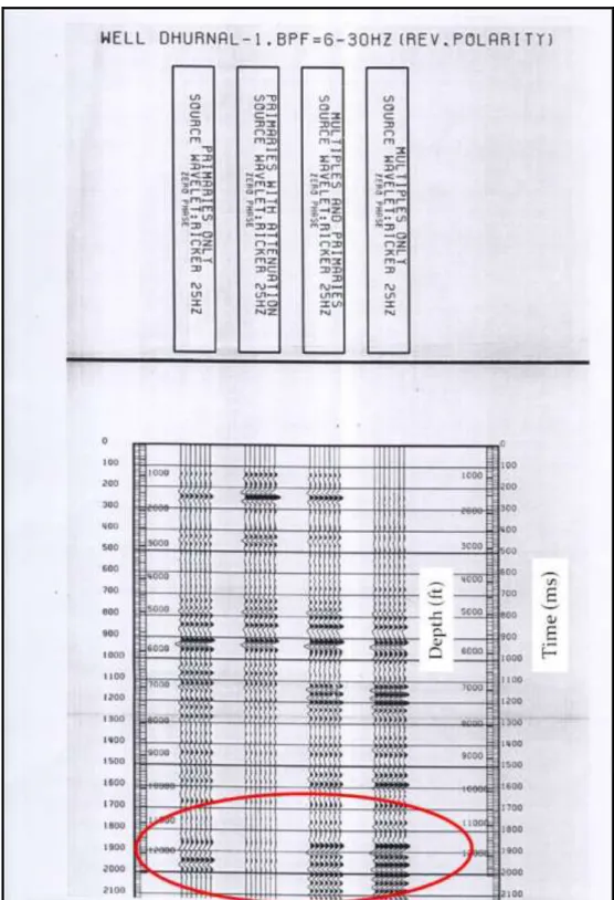
All seismic lines pertaining to the Dhurnal field were interpreted on workstation. Top of Miocene, Eocene, Paleocene, Permian and Infra Cambrian formations were identified on the basis of VSP data available on Dhurnal-1 well (Figure 2.1).
Top Eocene level was interpreted on seismic profiles of the study area after mistie adjustment. Below the Miocene group, the Eocene stratigraphic unit can be recognized throughout on the basis of distinctive seismic signatures having strong, continuous reflector of moderate to high amplitude.
13
Figure 2.1: Vertical seismic profile (VSP) of Dhurnal-1 well used for horizon identification. The
vertical panels above show the different processing levels. The red circle indicates the Eocene level which is the main reservoir in the Dhurnal field (Source: OPL).
14
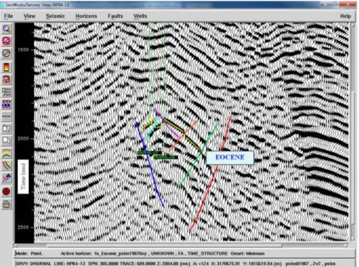
This reservoir horizon was then interpreted on each and every line present in the study area. Figures 2.2, 2.3, 2.4, 2.5, 2.6 and 2.7 are a few examples of horizon and fault interpretation.
Figure 2.2: Horizon interpretation on seismic line NP84-13 (1987 data). Yellow color shows
15
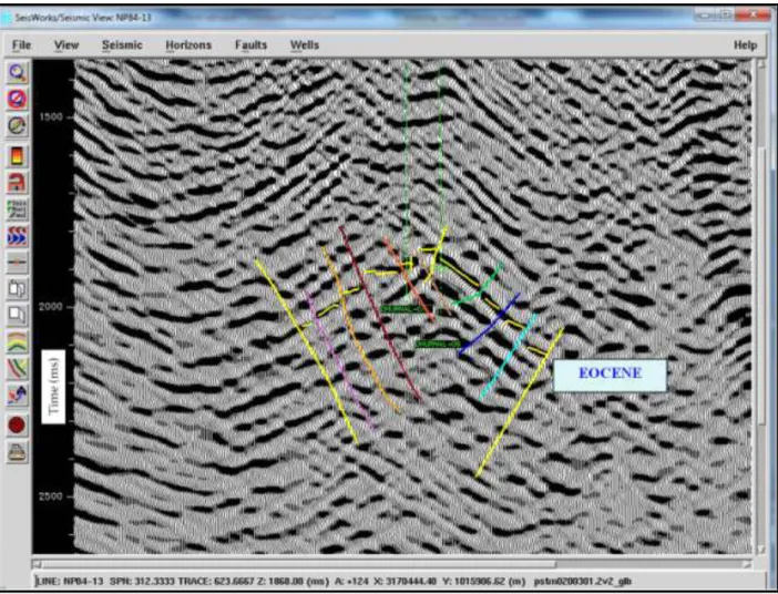
Figure 2.3: Horizon interpretation on seismic line NP84-13 (2003 data). Yellow color shows
16
Figure 2.4: Horizon interpretation on seismic line NP84-10 (1987 data). Yellow color shows
Eocene reflector and the rest of colors indicate fault interpretation.
Figure 2.5: Horizon interpretation on strike line NP84-52 (2003 data). The Eocene reflector is
marked and fault interpretation is also visible in this section. The inset map shows the location of this line highlighted by red.
17
Figure 2.6: Composite line passing through D-3 and D-6 wells (1987 data). This display clearly
indicates downthrown block at the reservoir level on line NP84-13. Eocene level is displayed by yellow color. The inset map shows the location of these line highlighted by red.
18
Figure 2.7: Composite line passing through D-3 and D-6 wells (2003 data). This display clearly
indicates the presence of anticlinal feature at reservoir level on line NP84-13. Eocene level is displayed by yellow color. The inset map shows the location of these lines highlighted by red.
19
Figure 2.8: Time structure map at Top Eocene level based on 1987 reprocessed PSTM data. The
black-colored time contours show that a downthrown block exists between D-1 and D-6 wells. The fault polygons are represented as grey where the fault arrows indicate a thrust regime and purple lines are the Dhurnal mining lease.
Figure 2.9: Time structure map at Top Eocene level based on 2003 reprocessed PSTM data.
According to black-colored time contour values, a pop-up anticlinal structure separates D-1 and D-6 wells. The fault polygons are represented as grey where the fault arrows indicate a thrust regime and purple lines are the Dhurnal mining lease.
20
2.1.1 Comparison of results of 2D interpretation based on 1987 and 2003 processed data
Figure 2.8 indicates lack of presence of any new structure between D-1 and D-6 wells. There is a downthrown block separating the two wells and the faults trend shows that the wells have been drilled at the optimum locations, and that there is no more structural anticlines undrilled in this area. So according to this interpretation, Dhurnal oil field lacks any further drillable hydrocarbon potential.
Figure 2.9 reveals that a pop-up anticlinal structure exists between D-1 and D-6 wells and has an aerial closure of 174 acres (0.704 sq. kms). Attic hydrocarbons may be present at this up-dip area that can be recovered by side-tracking D-1 well or drilling a new well.
The interpretation results clearly verified the major difference in the structural configuration of the two different seismic processing. The up-dip potential mapped on 2003 data confirmed that the anomaly observed on one seismic line does actually extend in the study area and had significant importance that cannot be neglected.
Therefore, in order to identify the reason behind this major discrepancy, a detailed and comprehensive analysis of the two different processing/reprocessing was carried out.
2.2 Seismic data processing/reprocessing
About 352 L.km of seismic data of two vintages by AMOCO (1972), OXY (1984) was processed up to PSTM level, at Golden Geophysical in 1987. The same 2D data set with addition of 17 L.km of OPI (2001) was reprocessed up to PSTM by PGS, Cairo in 2003. The reprocessing objective was to enhance/improve the clarity of minor faults, which had indicated compartmentalization.
The processing/reprocessing sequences of these two campaigns were analysed in detail by me. It was important to find out why this reprocessing (2003) differed from the old (1987) processing. Comparison of the two processing parameters showed that the difference in structural configuration was actually caused by the velocity modeling.
21
These reprocessing results were interpreted and demonstrated in the figure below:
Figure 2.10: Comparison of old 1987 and new 2003 processing/reprocessing of PSTM data
showing the presence of pop-up anticline in 2003 data. However, a downthrown block is observed exactly at the same shot point location on 1987 data.
2.2.1 Comparison of the two processing/reprocessing
Detailed review of the two processing sequences reveals that the major factor which may affect the sub-surface geometry was the dense seismic velocity analysis carried out on 2003 data. Apart from this, there was no significant difference in the processing parameters.
2.3 Velocity analysis
As mentioned earlier, velocity analysis is probably the most critical and important stage. On the 1987 data, velocity analysis was done on a 1 km grid (Figure 2.11), whereas, grid spacing used on 2003 data was 0.5 km (Figure 2.12). In my view, the closed grid interval enhanced the structural configuration and clarification of fault geometry. The 2003 PSTM time data showed
22
some changes in fault interpretation (Figure 2.12) and further improved the structure significantly.
Figure 2.11: Sparse velocity picking on old 1987 data showing vertical velocity panels at the top
of the seismic section. In this case, the velocity grid is 1 km apart displaying the zone of interest as a downthrown block between D-1 and D-6 wells.
23
Figure 2.12: Detailed velocity picking on 2003 data showing vertical velocity panels at the top
of the seismic section. In this case, the velocity grid is 0.5 km apart displaying a pop-up anticlinal structure (an up-thrust block) between D-1 and D-6 wells.
24
The velocity model is generated utilizing the root mean square (RMS) velocities provided at fixed CDP intervals on PSTM hard copy sections of the two data sets. These velocities were calculated and computed at the interpreted two way time of Top Eocene horizon. This velocity information was then imported to OpenWorks® and velocity maps were constructed using ZMap Plus™ software (Figures 2.13 and 2.14).
Figure 2.13: Velocity map based on 1987 data showing a velocity anomaly in the south of D-1
and D-6 wells. Black contours represent velocity trend (meter/second) in the area and purple lines are the Dhurnal mining lease.
25
Figure 2.14: Velocity map based on 2003 data showing a velocity anomaly over the apex of
Dhurnal structure. Black contours represent velocity trend (meter/second) in the area and purple lines are the Dhurnal mining lease.
2.3.1 Comparison of results of velocity analysis of 1987 and 2003 data
Figure 2.13 shows that the velocity anomaly was observed in the south of D-1 and D-6 wells. This shift in velocity anomaly from the apex of the Dhurnal structure was contradicting the structural configuration observed on Time structure map as flank of Dhurnal structure can be clearly seen on seismic lines and time map.
Whereas Figure 2.14 reveals the development of a velocity anomaly over the apex of Dhurnal structure which was due to dense velocity grid. This velocity anomaly seems to be fairly consistent with the geology of Dhurnal structure.
26
The velocity grids of 1987 and 2003 data were further merged with respective time grids to construct depth structure maps (Figures 2.15 and 2.16). Both single and dual grid operations were performed in ZMAP Plus™ software.
Figure 2.15: Depth map based on 1987 data showing lack of presence of any structural high
between D-1 and D-6 wells. The depth contours are drawn in black, fault polygons are represented as grey and purple lines are the Dhurnal mining lease.
27
Figure 2.16: Depth map based on 2003 data showing the presence of a structural high between
D-1 and D-6 wells. The depth contours are drawn in black, fault polygons are represented as grey and purple lines are the Dhurnal mining lease.
28
Chapter 3
3D seismic geophysical evaluation
3D seismic data was acquired in Dhurnal area in 2009 and had also been utilized and incorporated in my thesis to further verify the results presented in chapter 2.
3.1 3D Seismic data interpretation
In order to start my 3D seismic data interpretation, it was utmost important and vital to identify the target level on seismic data. Therefore, I constructed a synthetic seismogram of Dhurnal-1 well utilizing SynTool™ (LandMark) software. SynTool™ software allowed me to tie time data (the seismic data) to depth data (the well data) by integrating over the velocity profile.
A reflectivity series was generated by using sonic and density logs of Dhurnal-1 well. These reflection coefficients were convolved with an extracted seismic wavelet to produce a synthetic seismic trace. I extracted this wavelet from seismic because it gave the consistency in phase and frequency with actual seismic data (Figure 3.1). Therefore, it increased my level of confidence of horizon identification and interpretation. The synthetic seismogram was then compared with the actual seismic traces by displaying it over the seismic section at the Dhurnal-1 well location (Figure 3.2).
29
Figure 3.1: Characteristics of extracted wavelet (generated using SynTool™ software). The
30
Figure 3.2: Geo-seismic calibration showing the synthetic seismogram displayed over the real
seismic section to identify Eocene reflector. A reasonable well to seismic tie can be observed in the figure.
Same reservoir horizon (Top Eocene level) was interpreted on 3D data volume using SuperSeis® module of LandMark interpretation software. The horizon interpretation was imported to ZMap Plus™ software for generating two way time (Figure 3.3) and depth maps (Figure 3.4).
31
Figure 3.3: Time map at Top Eocene level based on 3D data confirms the existence of structural
high between D-1 and D-6 wells. The aerial closure of this anticline is 143 acres (dark green polygon) whereas the total area of Dhurnal structure comes out to be 3422 acres.
32
Figure 3.4: Depth map at Top Eocene level based on 3D data showing up-dip area between the
D-1 and D-6 wells. The color bar shows yellow as shallowest and blue as deepest. The depth contours are drawn in black, fault polygons are represented as grey and purple lines are the Dhurnal mining lease.
3.2 Results of 3D geophysical analysis
3D interpretation confirmed the presence of pop-up anticline/structural high between 1 and D-6 wells with negligible difference in aerial closure of the structure.
The confidence level on 2D geophysical results was enhanced after 3D interpretation as the seismic information was available at every 25 m for the entire study area, aiding in accurately mapping the structural complexities and the remaining up-dip potential of the Dhurnal field. Moreover, 3D PSTM time migrated data improved subsurface image delineating subtle subsurface features.
33
CHAPTER 4
4.1 Discussion
Comprehensive processing/reprocessing analysis of the available 2D seismic data sets confirmed that velocity was the most significant parameter of seismic data processing and played a vital role in delineating subtle sub-surface structures. Figure 2.9 shows the existence of pop-up anticline on 2003 seismic section, whereas, there is no such feature observed on the 1987 seismic section. This structure observed on line number NP84-13 was further confirmed in a planar view through detail 2D seismic data interpretation. Velocity modeling of the old and new 2D processed/reprocessed data was carried out to identify the possible cause of this structural disparity. The results indicated that the dense velocity picking on 2003 data led to the delineation of this subtle structure.
These findings were further confirmed by detailed 3D seismic data interpretation. The results of 3D interpretation revealed that the dense velocity model used in 2003 data was the most appropriate in this area. Also, structural configuration had been modified at Eocene level and confirmed the presence of up-dip potential as already delineated on 2003 velocity model. In a nutshell, my study indicates that there are sharp velocity changes (2003 data) that aided in resolving small-scale sub-surface structures which were missed due to coarse CDP spacing (1987 data) of velocity analysis.
Therefore, it is suggested that the delineated 143-174 acres up-dip area having attic recoverable hydrocarbons can be drained by sidetracking Dhurnal-1well about 225 meters towards southeast or drill a new well.
34
4.2 Conclusions
The interpretation of seismic data together with surface geological information indicates that the structural patterns in the Dhurnal oil field developed as a consequence of compressional tectonics. A pop-up anticlinal structure was delineated between D-1 and D-6 wells, due to close spacing of the velocity grid which highlights the importance of velocity analysis in seismic data processing. The size of the structure delineated in this research comes out to be 143 acres based on 3D mapping. However, the cumulative reserve estimation is about 1 million barrels of oil, which reflects on the significance and economic value of this structure.
Dhurnal-1 and Dhurnal-6 are in different compartments at the level of Eocene limestone. For all drilled reservoirs except Eocene, Dhurnal-6 is located at the crestal position. Therefore, the chances of having un-drained deeper potential or bypassed hydrocarbons in these reservoirs are minimal.
Hence, it is concluded that the dense velocity analysis is of key importance for the processing done for future field development.
35
References
Ahmed R, Ali SM and Ahmed J (1994). Review of Petroleum Occurrence and Prospects of Pakistan with special reference to adjoining basins of India, Afghanistan and Iran. Pakistan
Journal of Hydrocarbon Research. Vol 6 (7 – 18).
Davies LM and Pinfold E (1937). The Eocene beds of the Punjab Salt Range: in Shah, 1977, eds., Stratigraphy of Pakistan. Geological Survey of Pakistan. Mem 12.
Iqbal M and Ali SM (2001). Correlation of structural lineaments with oil discoveries in Potwar Sub-basin, Pakistan. Pakistan Journal of Hydrocarbon Research. Vol 12 (73 – 80).
Kazmi HA and Jan QA (1997). Geology and Tectonics of Pakistan.
Lillie RJ and Yousaf M (1986). Modern analogs for some midcrustal reflections observed beneath collisional mountain belts, in Barazangi M and Brown L, eds., Reflection seismology: the continental crust. American Geophysical Union Geodynamics Series. Vol 14 (55 – 65).
Molnar P and Tapponnier P (1975). Cenozoic tectonics of Asia: Effect of a continental collision.
Science. Vol 189 (419 – 426).
Pascoe EH (1959). A manual of the geology of India and Burma: in Shah, 1977, eds., Stratigraphy of Pakistan. Geological Survey of Pakistan. Mem 12.
Patriat P and Achache J (1984). Indian-Eurasian collisional chronology and its implications for crustal shortening and driving mechanism of plates. Nature 311 (15 – 621).
Pilgrim GE (1913). The correlation of the Siwaliks with mammal horizons of Europe: in Shah, 1977, eds., Stratigraphy of Pakistan. Geological Survey of Pakistan. Mem 12.
36
Pinfold ES (1918). Notes on structure and stratigraphy in the north-west Punjab: in Shah, 1977, eds., Stratigraphy of Pakistan. Geological Survey of Pakistan. Mem 12.
Porth H and Raza HA (1990). On the geology and hydrocarbon prospects of Potwar depression and adjoining sedimentary areas, Indus Basin, Pakistan. HDIP-BGR unpublished report. Pakistan Energy Year Book (2006).
Powell C (1979). A speculative tectonics history of Pakistan and surroundings: some constraints from the Indian Ocean, in Farah A., and DeJong, KA, eds., Geodynamics of Pakistan. Geological
Survey of Pakistan (1 – 24).
Raza HA, Ahmed R, Alam S and Ali SM (1989). Petroleum zones of Pakistan. Pakistan Journal
of Hydrocarbon Research. Vol 1, No 2 (1 – 19).
Sclater JG and Fisher (1974). Evolution of the east central Indian Ocean with emphasis on the tectonic setting of the Ninety East Range. Geological Society American Bulletin.
Seismic data processing report on OPI 2D land pre-stack depth migration in the Dhurnal field (2003). Petroleum Geo-services Data Processing, Cairo.
Twyford I (2010). Seismic Data Processing Report Dhurnal 3D, Pakistan. Fugro Seismic Imaging Limited.
Tidigare utgivna publikationer i serien ISSN 1650-6553
Nr 1 Geomorphological mapping and hazard assessment of alpine areas in
Vorarlberg, Austria, Marcus Gustavsson
Nr 2 Verification of the Turbulence Index used at SMHI, Stefan Bergman
Nr 3 Forecasting the next day’s maximum and minimum temperature in Vancouver,
Canada by using artificial neural network models, Magnus Nilsson
Nr 4 The tectonic history of the Skyttorp-Vattholma fault zone, south-central Sweden,
Anna Victoria Engström
Nr 5 Investigation on Surface energy fluxes and their relationship to synoptic weather
patterns on Storglaciären, northern Sweden, Yvonne Kramer
Nr 256 Water quality in the Koga Irrigation Project, Ethiopia: A snapshot of general
quality parameters.Vattenkvalitet i konstbevattningsprojektet i Koga, Etiopien: En överblick av allmänna kvalitetsparametrar. Simon Eriksson, Mars 2013
Nr 257 3D Processing of Seismic Data from the Ketzin CO2 Storage Site, Germany.
Jawwad Ashraf Qureshi, April 2013
Nr 258 Investigations of Manual and Satellite Observations of Snow in Järämä (North
Sweden) Daniel Pinto, May 2013
Nr 259 Jämförande studie av två parameterskattningsmetoder i ett grundvattenmagasin.
Comparative study of two parameter estimation methods in a groundwater aquifer.
Stefan Eriksson, May 2013
Nr 260 Case Study of Uncertainties Connected to Long-term Correction of Wind
Observations. Elisabeth Saarnak, May 2013
Nr 261Variability and change in Koga reservoir volume, Blue Nile, Ethiopia . Variabilitet
och förändring i Koga dammens vattenvolym, Blå Nilen, Etiopien. Benjamin Reynolds, May 2013
Nr 262 Meteorological Investigation of Preconditions for Extreme-Scale Wind Turbines
in Scandinavia. Christoffer Hallgren, May 2013
Nr 263 Application of the Reflection Seismic Method in Monitoring CO2 Injection in a
Deep Saline Aquifer in the Baltic Sea. Saba Joodaki, May 2013
Nr 264 A climatological study of Clear Air Turbulence over the North Atlantic.
Leon Lee, June 2013
Nr 265 Elastic Anisotropy of Deformation Zones in both Seismic and Ultrasonic
Frequencies: An Example from the Bergslagen Region, Eastern Sweden. Pouya Ahmadi,
June 2013