Analysis of selenium cycling and remediation in Colorado's Lower Arkansas River Valley using field methods and numerical modeling

(1)

THESIS

ANALYSIS OF SELENIUM CYCLING AND REMEDIATION

IN COLORADO’S LOWER ARKANSAS RIVER VALLEY

USING FIELD METHODS AND NUMERICAL MODELING

Submitted by Erica C. Romero

Department of Civil and Environmental Engineering

In partial fulfillment of the requirements For the Degree of Master of Science

Colorado State University Fort Collins, Colorado

Fall 2016

Master’s Committee:

Advisor: Timothy K. Gates Co-Advisor: Ryan T. Bailey Dana L. K. Hoag

(2)

(3)

ABSTRACT

ANALYSIS OF SELENIUM CYCLING AND REMEDIATION IN COLORADO’S LOWER ARKANSAS RIVER VALLEY USING FIELD METHODS AND NUMERICAL MODELING

Groundwater and surface water concentrations of selenium (Se) threaten aquatic life and livestock as well as exceed regulatory standards in Colorado’s Lower Arkansas River Valley (LARV). Se is naturally present in surface shale, weathered shale, and bedrock shale in the region. Excess nitrate (NO3) from irrigated agricultural practices oxidizes Se from seleno-pyrite

present in shale and inhibits its chemical reduction to less toxic forms. Irrigation-induced return flows and evapotranspiration induce high concentrations of Se in the alluvial groundwater resulting in substantial nonpoint source loads to the stream system.

This research uses three main components to address the need to better describe and find solutions to the problem of Se pollution in the LARV: (1) Se data collection in streams to characterize solute and sediment concentrations, (2) development of a conceptual model of in-stream Se reactions, and (3) application of existing calibrated groundwater models to explore alternative Se remediation strategies. Data in the form of Se solute samples, Se sediment samples, and related water properties were collected during four different sampling events in 2013 and 2014 at several locations in the stream network in an effort to understand the various species of Se and how they cycle through the surface water environment. A conceptual representation of the major chemical reactions of Se in the water column and sediments of streams was described and incorporated into the OTIS (One-Dimensional Transport with Inflow and Storage) computational model of stream reactive transport for future coupling to the

(4)

MODFLOW-UZF and RT3D-UZF groundwater models. The new version of OTIS, now called OTIS-MULTI, allows for simulation of the cycling of multiple Se species in the river

environment. Lastly, five best management practices (BMPs) were tested using MODFLOW-UZF and RT3D-MODFLOW-UZF: improved irrigation efficiency (reduced irrigation), lining or sealing of canals to reduce seepage, lease fallowing of irrigated fields, improved fertilizer management (reduced fertilizer), and enhancement of riparian buffers. The impact of each of these BMPs on Se loading to the stream network was evaluated individually over three scenarios in which the adaption of each BMP is incrementally increased. In addition, various combinations of three and four BMPs were simulated and compared.

Water samples gathered from the Arkansas River had total dissolved Se concentrations ranging from 6.1 to 32 g/L (ICP method), compared to the Colorado chronic standard of 4.6 g/L, while concentrations in samples gathered from tributaries ranged from 6.04 to 29 g/L (ICP method). The groundwater and drinking water standard from the National Primary

Drinking Water Regulations for selenium is 50 g/L (USEPA, 2016). Concentrations of total Se (sorbed, reduced, and organic) in river bed sediments ranged from 0.16 to 0.36 g/g with

concentrations in river bank samples ranging from 0.26 to 1.78 g/g. About 70 to 80% of Se in bed and bank sediments was found to be in a reduced or organic form. Analysis also reveals statistically significant high correlations of 0.70-1.00 between sorbed SeO3 (bed sediment (µg/g)

and sorbed SeO4 (bed sediment) (µg/g); sorbed SeO3 (bed sediment (µg/g) and estimated

precipitated and organic Se (bed sediment) (µg/g); sorbed SeO4 (bed sediment) (µg/g) and

estimated precipitated and organic Se (bed sediment) (µg/g); ammonium (mg/L) and nitrite-nitrogen (NO2-N) (mg/L); NO3-N (mg/L) and total dissolved Se (µg/L); and sorbed SeO4 (bank

(5)

(µg/g). The conceptualization of key Se reactions was incorporated into OTIS-MULTI and must now be tested and calibrated for future application. The groundwater model results indicate that the individual BMP scenarios that most effectively decrease Se total mass loadings to the Arkansas River and its tributaries are: lease fallowing, resulting in a 15% decrease in predicted mass loading; reduced irrigation, with an 11% decrease; canal lining or sealing, with a 10% decrease; enhanced riparian buffer, with a 7% decrease; and reduced fertilizer, with a 3% decrease. In comparison, a BMP combination of lease fallowing, canal lining or sealing, enhanced riparian buffer, and reduced fertilizer was predicted to reduce loads by 46% and a combination of reduced irrigation, canal lining or sealing, enhanced riparian buffer, and reduced fertilizer by 44%. The hope, to be proven by future investigations, is that these reduced loads will contribute to lower concentrations in the river system.

(6)

ACKNOWLEDGMENTS

I am very grateful to the Nonpoint Source Program of the Water Quality Control Division of the Colorado Department of Public Health and Environment and to the Colorado Agricultural Experiment Station for their financial support of this work. I would like to thank my advisor, Dr. Timothy K. Gates, and co-advisor, Dr. Ryan T. Bailey for the opportunity to work on this project and for all of their advice and help. I am grateful to Dr. Dana Hoag for the chance to work with him on this project and to learn more about an alternative perspective. I would like especially to thank to my fellow graduate and undergraduate students who worked and helped me on this project: Misti Sharp, Mike Weber, Corey Wallace, Cale Mages, Brent Heesemann, Alex Huizenga, Caroline Draper and Chaz Meyers. I am very grateful to Brent Heesemann for his help in performing the statistical analysis on the collected field data, for creating Figure 3 of this thesis for shared use, and for helping me with other numerous questions along the way. Special thanks are extended to Misti Sharp for keeping me as positive as possible while working on this thesis (she is the best study buddy ever). My other friends’ encouragements in my times of need are much appreciated. Most of all, I would like to thank Carl, my husband, and my family for their support and words of wisdom in helping me complete my MS degree.

(7)

TABLE OF CONTENTS

Abstract ... ii

Acknowledgments... v

List of Tables ... viii

List of Figures ... ix

Chapter 1: Introduction ... 1

1.1 Background and Problem Statement ... 1

1.2 Objectives ... 5

1.3 Study Region ... 7

Chapter 2: Literature Review ... 10

2.1 Selenium Chemistry ... 10

2.2 Sources of Selenium ... 11

2.3 Selenium Cycling in Soil and Water ... 12

2.4 Field Sampling of Selenium in Water and Sediments ... 15

2.5 Se Modeling ... 21

2.5.1 Modeling Se in Groundwater (Saturated and Unsaturated) ... 21

2.5.2 Modeling Se in Surface Water and Sediments ... 24

2.6 CSU Modeling of Salinity and Se in the Arkansas River Valley ... 24

2.7 Best Management Practices for Se ... 32

2.7.1 Enhanced Riparian Buffer Zones ... 32

2.7.2 Reduced Fertilizer Application ... 34

2.7.3 Increased Irrigation Efficiency ... 35

2.7.4 Canal Sealing ... 37

2.7.5 Lease Fallowing ... 38

Chapter 3: Methods ... 40

3.1 Collection and Analysis of Stream Water and Sediment Samples ... 40

3.1.1 Field Sampling and Measurements ... 41

3.1.1.1 Bank and Sediment Sampling ... 44

(8)

3.1.1.3 Filtered Water Sampling ... 46

3.1.1.4 Chla Sampling ... 47

3.1.1.5 Flow Measurements with ADVs ... 47

3.1.1.6 In-Situ Measurements of Water Properties ... 48

3.1.1.7 Surveys of Stream Cross-Section Geometry ... 49

3.1.2 Lab Analysis Summary ... 51

3.2 Conceptual Model for Se Cycling in Surface Water ... 53

3.3 Groundwater Modeling: Description of BMPs and Implementation in MODLFOW-UZF and UZF-RT3D ... 54

Chapter 4: Results and Discussion ... 60

4.1 Analysis of Stream Water and Sediment Samples ... 60

4.1.1 Residual, Sorbed and Dissolved Se in Stream Banks and Sediments... 60

4.1.2 Database Compilation of Unfiltered and Filtered Water Measurements ... 64

4.1.3 Chla Results ... 64

4.1.4 Flow Measurements with ADVs ... 64

4.1.5 Pearson Correlation of Bank and Bed Sediment Concentrations, Stream Water Concentrations, and In-Situ Measurements of Water Properties ... 66

4.2 Surface Water Modeling ... 71

4.2.1 Se Surface Water Conceptual Model ... 71

4.2.2 Selenium Equations for OTIS-MULTI ... 73

4.3 Simulating the BMPs with MODFLOW-UZF and UZF-RT3D ... 79

4.3.1 Se Mass Loadings ... 79

4.3.2 Se Groundwater Concentrations ... 90

Chapter 5: Summary, Conclusions, and Recommendations ... 98

References ... 104

Appendix A: Field Sample Locations and Field Notes ... 112

Appendix B: Field Data Results ... 136

(9)

LIST OF TABLES

Table 2-1. Summary of characteristics included in Se numerical modeling studies (modified

from Bailey 2012) ... 22

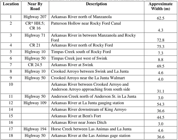
Table 3-1. Locations and characteristics of measurement locations on the Arkansas River and its

tributaries ... 41

Table 3-2. Locations measured for all trips during March 2013 – March 2014. An X indicates

the location was sampled. ... 42

Table 3-3. Five individual BMP scenarios and four sets of combined BMPs simulated at three

different levels of intensity. ... 58

Table 4-1. Averages of residual (precipitated and organic) and sorbed Se concentrations in the

stream banks and bed sediments of the Arkansas River and the tributaries sorted for each

sampling trip. ... 60

Table 4-2. Summary of ADV measurements of Q compared to Q measured at nearby gauging

stations. ... 66

Table 4-3. Pearson correlation table for Se concentrations in samples taken from both the

Arkansas River and the tributaries. ... 68

Table 4-4. Pearson correlation table for nutrient and Se concentrations in samples taken from

both the Arkansas River and the tributaries. ... 70

Table 4-5. Pearson correlation table for Se concentrations in samples taken from only the

Arkansas River. ... 70

Table 4-6. Percent decreases (from Baseline) for six command areas and the outside (non–

irrigated land). The green and yellow are small positive or negative final percent differences corresponding to a decrease in the Se concentration percent difference. Red and orange cells are larger positive percent differences and correspond to an increase in the Se concentration percent decrease. ... 97

Table 5-1. Spatial variability of dissolved Se concentrations in g/L for each trip, the river, and

tributary data. ... 99

Table B-1. Se laboratory results ... 136 Table B-2. Nitrogen, phosphorous, and uranium laboratory results ... 137 Table B-3. All sorbed and residual (precipitated and organic Se) data for all trips sorted by

sample point in the Arkansas River and by location... 140

Table B-4. All sorbed and residual (precipitated and organic Se) data for all trips sorted by

(10)

LIST OF FIGURES

Figure 1-1. Abnormal embryos from eggs of aquatic birds at Kesterson from Ohlendorf (1986).

The image on the left shows an American coot with truncated feet. The image on the right is a Black-necked stilt with abnormalities of the lower beak, poorly developed eyes, and no legs or one wing. ... 2

Figure 1-2. The Lower Arkansas River Valley in Colorado with two CSU study regions (black

boxes) within Segments 1B and 1C of the Arkansas River ... 4

Figure 1-3. The USR showing the locations of the previous groundwater and surface water

monitoring sites as well as the surface water locations sampled in this study (bold) in the

Arkansas River and its tributaries. ... 9

Figure 2-1. Images of the following samplers: (A) Depth-integrating wading type US DH-48;

(B) depth-integrating suspended type US D-77; (C) point-integrating suspended sediment US P-72; (D) pumping sampler (www.geoscientific.com); (E) bed-material US BMH-60; and (F) bedload sampler US BL-84 (Depth-Integrating Samplers, 2009 for A-C and E-F) ... 17

Figure 3-1. Stream measurement locations in the USR for March 2013-March 2014 ... 40 Figure 3-2. Location 1, a cross-section on the Arkansas River near Manzanola (facing

downstream). Blue arrows indicate where sediment samples were collected (April 2014). ... 44

Figure 3-3. The sleeves and caps used for collecting bed and bank sediment samples in the

Arkansas River and its tributaries. ... 45

Figure 3-4. (A) A churn used for averaging the point suspended sediment samples into a

cross-section averaged sample from

http://pubs.usgs.gov/of/2000/ofr00-213/manual_eng/prepare.html#fig4. (B) DH48 sediment sampler used for shallow water and suspended sediment. Image from http://www.benmeadows.com/depth-integrated-sediment-samplers_36816467/ ... 46

Figure 3-5. (A) A close up of the FlowTracker (www.sontek.com) and (B) the FlowTracker and

wading rod being used to measure flow. ... 48

Figure 3-6. An YSI 600 QS Multiparmeter Sampling System used for in-situ measurements of

water properties. ... 49

Figure 3-7. Surveying equipment including (A) the base unit (left) and rover (right) and (B) the

Tesla data collector

(http://www.gim-international.com/news/id6214-Juniper_to_Manufacture_Topcon_Tesla.html). ... 50

Figure 4-1. Percentages of dissolved Se species in the water and of sorbed Se species compared

to residual Se in the bank and bed sediments for samples from the Arkansas River for Trip 2. .. 63

Figure 4-2. Percentages of dissolved Se species in the water and of sorbed Se species compared

to residual Se in the bank and bed sediments for samples from the tributaries for Trip 2. ... 63

Figure 4-3. Se cycling in surface water where the dominant direction of reactions are shown but

(11)

Figure 4-4. The spatial distribution of cumulative simulated Se mass loadings over the simulated

time period for the Baseline scenario... 79

Figure 4-5. The spatial distribution of cumulative Se mass loading over the simulation time

period for the LF25 BMP scenario. ... 80

Figure 4-6. The spatial distribution of cumulative Se mass loading differences from the Baseline

over the simulation time period for BMP scenarios LF5, LF15, and LF25... 81

over the simulation period for basic, intermediate, and aggressive combined BMP scenarios. ... 82

over the simulation period for all individual aggressive BMPs and for two combined BMPs involving a change in the amount of water applied ... 83

Figure 4-9. Baseline total Se mass to the Arkansas River in kg/day for the entire simulation

time 38 years ... 84

Figure 4-10. Time series of simulated differences in total Se mass to the Arkansas River and

tributaries from the Baseline for (A) reduced irrigation (RI), (B) canal sealing (CS), (C) land fallowing (LF), (D) reduced fertilizer (RF), (E) enhanced riparian buffer zone (ERB), and (F-G) combination BMP scenarios. Scenario (F) implements RI, CS, and RF BMPs simultaneously while Scenario (G) implements LF, CS, RF, and ERB BMPs simultaneously. ... 86

Figure 4-11. Percent decrease in simulated total dissolved Se mass loadings directly to the

Arkansas River for individual and combined BMPs. Abbreviations for basic, intermediate, and aggressive are the following bas., int., and agg. respectively. ... 89

Figure 4-12. Percent decrease in total dissolved Se total mass loadings to the Arkansas River

plus the tributaries (Crooked Arroyo and Timpas Creek) in red and directly to the Arkansas River alone in blue for individual and combined BMPs. Abbreviations for basic, intermediate, and aggressive are the following bas., int., and agg. respectively. ... 90

Figure 4-13. The canal command areas of the Upstream Study Region ... 91 Figure 4-14. Time series percent decrease of average 4 concentrations for the Rocky Ford

Highline Canal, Otero Canal, Catlin Canal, Rocky Ford Ditch, Fort Lyon Canal, Holbrook Canal, Outside region ... 93

Figure B-1. Trip 1 in the Arkansas River: percentages of dissolved Se species in the water and

sorbed Se species compared to residual Se ... 146

Figure B-2. Trip 1 in the Tributaries: percentages of dissolved Se species in the water and

sorbed Se species ... 146

(12)

Figure C-1. The spatial distribution of temporally-averaged simulated Se mass loading

differences from the Baseline for reduced irrigation scenarios ... 150

differences from the Baseline for canal sealing scenarios ... 151

differences from the Baseline for reduced fertilizer scenarios ... 152

differences from the Baseline for enhanced riparian buffer scenarios ... 153

differences from the Baseline for three combination reduced irrigation scenarios ... 154

differences from the Baseline for three combination lease fallowing scenarios ... 155

(13)

Chapter 1: Introduction

1.1 Background and Problem Statement

Selenium (Se) is a required micro-nutrient for life; however, at high levels Se is toxic to humans, livestock, and aquatic species alike. For humans, the recommended range for dietary health lies between 40-400 micrograms/day (μg/day) (Levander and Burk, 2006). Once intake exceeds 400 µg/day a person is susceptible to selenosis with symptoms of defective nails and skin, hair loss, unsteady gait, and paralysis according to the United States Agency for Toxic Substances & Disease Registry Toxicological Profile for Se (USHHS, 2003). Acute oral

exposure to high Se doses leads to nausea, vomiting and diarrhea, and sometimes cardiovascular symptoms (Lenz and Lens, 2009). For aquatic life, the toxic threshold for Se varies with regards to species and with the location where Se is measured, whether in water, soil, or tissue. The bioaccumulative nature of Se in the river system, especially in stagnant water areas, contributes to why different thresholds exist in different mediums. However, Hamilton (2004) suggests a toxicity threshold for fish near 3 µg/L and for sediment 4 µg/g as a general guide. When

organisms or specific fish species are in danger, the literature should be consulted to determine a more suitable toxicity threshold. Two other important factors to consider in determining an aquatic toxicity threshold is the location in a water system, whether in the lotic (streams and rivers) or lentic (backwaters, side channels, reservoirs) areas, as well as whether the fish in question are a cold water or warm water variety (Hamilton 2004). In the embryo-larval stages of life, terotogenesis will develop in wild birds and fish whose parents were exposed to high levels of Se (Lemly, 1999; Hamilton, 2004). The side effects of terotogenesis in fish include curvature of lumbar and the spine; deformity of the head, mouth, gill cover, and fin; as well as edema, and

(14)

An early documentation of Se toxicity to livestock due to high plant and soil

concentrations occurred in South Dakota in the middle 19th century (USHHS, 2003). Other investigations have been made, predominantly in the western United States. Of these areas, Kesterson Reservoir, CA was fed with high Se loadings from the irrigated soils of the San

Joaquin Valley. The examination of Kesterson Reservoir was documented in hundreds of reports and publications (Hamilton, 2004) potentially making it the most famous case of Se poisoning (Bailey, 2012). The wildlife most visually affected in the area were various specious of duck: embryos shown in Figure 1-1 (Ohlendorf et al., 1986; Hoffman et al., 1988).

Figure 1-1. Abnormal embryos from eggs of aquatic birds at Kesterson from Ohlendorf (1986). The image on the left shows an American coot with truncated feet. The image on the right is a Black-necked stilt with abnormalities of the lower beak, poorly developed eyes, and no legs or one wing.

Following the closure and capping of Kesterson Reservoir, Se loading still continues to the Central Valley, San Joaquin River, the San Joaquin-Sacramento Delta, and San Francisco Bay (Hamilton, 2004). Further mitigation measures may be necessary to prevent continued pollution downstream.

In Colorado, the Colorado River received Se in irrigation return flows, reported as early as 1935 by Williams and Byers (1935). The extent of the study of Se on the Colorado River ranges from the headwaters in Colorado to the Colorado River Delta in Mexico where elevated concentrations prevail (Garcia-Hernandez et al., 2001). Due to the evidence of

(15)

threshold-exceeded concentrations in biota documented in Garcia-Hernandez et al. (2001), suggestions have been made that the Colorado River water should be mixed with agricultural drainage water to reduce toxic thresholds, that wetlands should have an outflow to decrease organic carbon and thereby lower Se concentrations, and that no dredging should be allowed to reduce toxicity in fish.

Of primary consideration in the Colorado River in Colorado are endangered species including the Colorado pikeminnow (Ptychocheilus lucius) and razorback sucker (Xyrauchen texanus) (Osmundson et al., 2000). Osmundson et al. (2000) discusses the difficulty in quantifying the extent of the Se problem with a method that does not cause fish sacrifice. Muscle plugs were taken from the fish and analyzed by neutron activation. The average Se concentrations found in the muscle tissue of the Colorado pikeminnow exceeded the toxic threshold of 8 µg/g dry weight from 1994-1996 (Osmundson et al., 2000). Since the 1960s, advocates have called for the protection for endangered fish along Colorado River as described in Hamilton (2004). Hamilton (2004) also discusses a controversy over the threshold toxicity concentration for fish predominantly and he disproves the hypothesis that certain fish species may have evolved to live in Se-rich environments.

Due to phosphate mining, the Blackfoot River watershed of southeastern Idaho has been impacted by Se as described by sampling of water, surficial sediment, aquatic plants, aquatic invertebrates, and fish in nine streams in 2000 (Hamilton et al., 2002). Water samples only exceeded the national water quality standard of 5 μg/L for Se at two sites. Most creek samples contained the same amount of inorganic elements; however, Dry Valley Creek had high amounts of aluminum, copper, iron, and magnesium. The most serious of results were those of

(16)

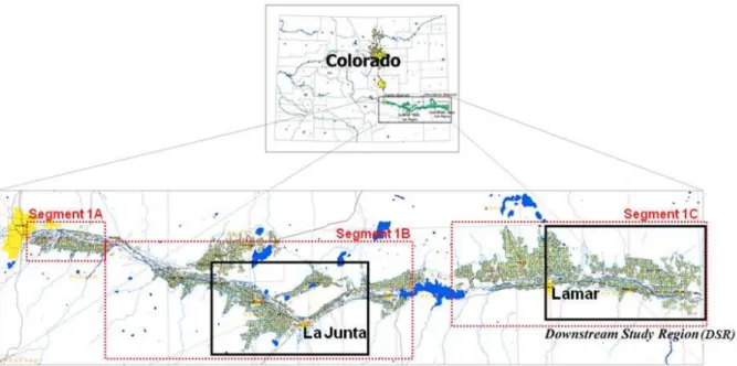
Se is also a serious issue in surface water and groundwater of the Lower Arkansas River Valley (LARV) in Colorado with potential toxic impacts on aquatic life and livestock since all three segments of the Lower Arkansas River were designated in 2004 as “water quality limited” with respect to Se and have been placed on the current Clean Water Act 303(d) list for total maximum daily loads (TMDL) development. Collected data indicate that Se concentrations are double the Colorado chronic standard of 4.6 μg/L for aquatic life in an Upstream Study Region (USR), which is shown in Figure 2 within Segment 1B of the river. The USR is named as such due to its location upstream of the John Martin Reservoir. More details on the data collection and analysis of Se in the region are discussed in Chapter 2. The affected segments of the river are designated by the Colorado Department of Public Health and the Environment (CDPHE) as COARLA01A (Segment 1A) COARLA01B (Segment 1B), and COARLA01C (Segment 1C) (Figure 2).

Figure 1-2. The Lower Arkansas River Valley in Colorado with two CSU study regions (black boxes) within Segments 1B and 1C of the Arkansas River

(17)

The Se problem in the LARV has developed over time since Se is naturally present in marine shale, which underlays and outcrops from the alluvial valley and is released from FeSe2

through reduction of oxidative species such as dissolved oxygen and NO3 into surface water and

groundwater (Fernandez-Martinez and Charlet, 2009). For over a hundred years, irrigated farming has been prevalent in the area, growing crops such as melons, corn, alfalfa, onions, grass, sorghum and others. The irrigation water, containing high amounts of dissolved oxygen and NO3,applied on the land has increased the dissolution of Se from weathered, bedrock, or

surficial shale deposits. More recently, due to the application of fertilizers for farming

productivity, the level of NO3 has increased in the groundwater and surface water of the LARV

thereby enhancing the dissolution of Se from shale via redox reactions (Bailey et al., 2012).

1.2 Objectives

To better address the problem of Se and N pollution in the LARV, the Nonpoint Source Program (NPS) of the Water Quality Control Division (WQCD) of the Colorado Department of Public Health and Environment (CDPHE) funded a project entitled “Identifying Arkansas River Selenium and Nitrogen Best Management” in 2012. A major aim was to use calibrated

groundwater and stream models to estimate current Se loadings to the Arkansas River and tributaries and to examine the potential for alternative best management practices (BMPs) to reduce Se loadings and consequently lower solute concentrations toward compliance with regulatory standards. Key stakeholders and water agencies are being engaged for their input on the feasibility and desirability of considered BMPs. Economic analysis of the costs and benefits of the alternative BMPs also is being conducted. An ultimate goal is to develop a plan for implementation of a pilot program to test the effectiveness of the BMPs identified to be most promising. A companion project, supported by the Water Quality Improvement Fund (WQIF),

(18)

provided supplemental funds not only for modeling but also for field data collection and analysis to characterize how Se and N are processed in the stream system.

A major goal of the research in the LARV is to create calibrated regional-scale

groundwater-surface water flow and reactive transport models that can be used to simulate the spatial and temporal distribution of Se and N concentrations in both the aquifer and the Arkansas River and its tributaries for characterization and for finding ways to lower these concentrations to meet regulatory and performance standards. The research presented in this thesis is important because it takes intermediate steps to reach this goal. The primary objectives are to:

1. Collect additional field data on Se concentrations and related water quality parameters in the Arkansas River and its tributaries to enhance the existing database and to inform both

groundwater and stream models,

2. Develop a conceptual model along with mathematical expressions of the major processes involved with Se cycling in the stream system for use in a computational model of reactive fate and transport, and

3. Use existing calibrated and tested groundwater flow and transport models to explore and rank alternative BMPs for abatement of Se loading in groundwater and, consequently, for lowering Se concentrations in the Arkansas River and its tributaries.

Background, methods, and results associated with meeting these objectives are documented herein. Chapter 2 provides a literature review, discussing the background of Se chemistry, sources of Se, field sampling of Se in water and soil, Se in the environment, Se modeling research, prior CSU characterization and modeling of Se in the LARV, and remediation strategies. Chapter 3 describes the methods of field collection, description of Se surface water

(19)

cycling relationships, and groundwater modeling of BMPs for mitigating Se loading to streams of the LARV. Results are presented and discussed in Chapter 4. Chapter 5 summarizes the research, presents major conclusions, and suggests future work.

1.3 Study Region

The USR in the LARV, where the current study focuses, extends from just west of

Manzanola, CO to near Las Animas, CO (Figure 1-2). Of the total 50,600 hectares (ha) (125,000 acres), 26,400 ha (65,300 acres) are irrigated lands which receive water from canals or pumping wells (Gates et al., 2009). As detailed in Gates et al., (2009), data have been collected focusing on Se and Se-related ions for both the USR and Downstream Study Region (DSR) extensively from 2003 to 2011. Monitoring of Se was implemented in the shallow unconfined alluvial aquifer and in the tributaries and drains of the Arkansas River. A total of 16 sampling events were conducted in the USR over the period June 2006 – May 2011. The routine surface water and groundwater samples were collected in 45 groundwater observation wells, four locations in tributaries and drains, and 10 locations along the river. Groundwater and surface water samples were collected for analysis of total dissolved Se concentration, dissolved uranium (U)

concentration, and major salt ion concentrations including sodium, potassium, magnesium, calcium, nitrate, sulfate, chloride, bicarbonate, carbonate, and boron. Water quality properties including pH, electrical conductivity (EC), temperature, dissolved oxygen (DO), and oxidation reduction potential (ORP) also were measured in-situ.

Data collection for the present study was based on the previous methods reported in Gates et al. (2009); however, a few key differences exist. In addition to gathering and analyzing water samples from the Arkansas River and its tributaries, sediment samples also were collected from the top 0.2 – 0.3 m of the channel bed and banks for analysis of sorbed and reduced (and

(20)

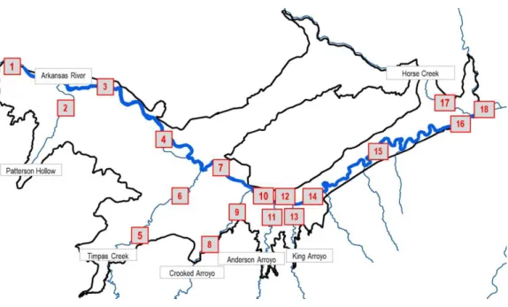
organic) Se. Three complete surface water and sediment sampling events were conducted in March 2013, June 2013, and March 2014 for analysis of total and dissolved Se concentrations, dissolved U concentrations, and the same specific related ions as reported in Gates et al. (2009). In March 2013, eight locations in the Arkansas River and seven locations in five different tributaries were sampled. In June 2013, nine locations in the Arkansas River and seven tributary locations were sampled. In March of 2014, four Arkansas River and four tributary locations were sampled. One abbreviated sampling event was conducted in August 2013 but, due to insufficient flows, could not be completed. Only three river and one tributary location were sampled during this event. The locations of previous groundwater and surface water monitoring sites compared to the current project monitoring locations are shown in Figure 1-3.

Key findings of Gates et al. (2009) were that the average measured Se concentration ( _� ) in the Arkansas River exceeds the CDPHE chronic standard of 4.6 µg/L (85th percentile) for aquatic habitat on average by a factor of about 2.5 to 3 in the USR. The livestock water standard also was substantially elevated with the averaged measured _� in groundwater at 57.7 µg/L, compared to the standard of 30 µg/L. The spatial and temporal variability is large, indicating varying management solutions may be needed.

Correlation was found to be moderate between _� and salinity as represented by total dissolved solids (TDS) and EC in both groundwater and surface water. Values of _� in

groundwater are strongly correlated with up-gradient distance to the identified near-surface shale ( _�) in the USR. High correlation exists between _� and the concentration of U ( _�) in

groundwater and surface water. The ratio of _� in groundwater to that in water diverted for irrigation from the river is too large to be explained by the evaporative concentration alone, implying oxidative dissolution of Se from geologic strata. Values of _� in groundwater are

(21)

strongly correlated to the concentration of nitrate ( ) indicating that NO3 enhances the

dissolution of Se from soil and rock and its retention in solution. Finally, threshold

concentration levels of roughly 10 mg/L for and 7 mg/L for DO appear to inhibit chemical reduction and promote oxidative dissolution from shale deposits as determined from analysis of the influence of and DO on the correlation of _� and _� with _�.

Figure 1-3. The USR showing the locations of the previous groundwater and surface water monitoring sites as well as the surface water locations sampled in this study (bold) in the Arkansas River and its tributaries.

(22)

Chapter 2: Literature Review

2.1 Selenium Chemistry

Se is a nonmetal with an atomic number of 34, relative mass of 78.971 and electron configuration [Ar] 3d10 4s2 4p4 as described by the Royal Society of Chemistry (Periodic Table-Selenium, 2014). The element is present in four main oxidation states (+VI), (+IV), (0), and (-II) in nature (Barceloux, 1999); in organic and inorganic forms; in solid, liquid, and gas phases; and in six stable isotopes (Lenz and Lens, 2009). The soluble oxyanions of Se are selenate (SeO4-2)

and selenite (SeO3-2). The fully oxidized Se(VI) form, SeO4-2, exists in solution as biselenate

(HSeO4-) or SeO4-2 (Seby et al., 2001); although, SeO4-2 is the dominant form at high redox

potentials and has low adsorption and precipitation capacities (Alemi, 1988; Balistrieri and Chao, 1987). The two forms of Se(IV) are SeO3-2 and the gas selenium dioxide, SeO2; SeO3-2 also can

exist as three weak acid species including H2SeO3, HSeO3-, or SeO32- depending on the pH of the

solution. SeO3-2 is the major species in the moderate redox potential range, and its mobility is

mainly governed by sorption/desorption processes on various solid surfaces such as metal hydroxides (Balistrieri and Chao, 1987; Papelis et al., 1995), clays (BarYosef and Meek, 1987), and organic matter (Gustafasson and Johnsson, 1994).

Non-soluble elemental Se or Se(0) occurs in the form of at least 11 allotropes, seven crystalline and four non-crystalline (Minaev et al., 2005). The final two oxidation states, (-II) and (-I), occur in a variety of metallic selenides and many organic compounds and are stable under strongly reducing conditions (Fernandez-Martinez and Charlet, 2009). Other forms of Se found in surface water, groundwater, or wastewater include non-volatile organic selenides such as seleno amino-acids and volatile methylated forms of selenides such as dimethylselenide (DMSe) and dimethyldiselenide (DMDSe) (Fernandez-Martinez and Charlet, 2009).

(23)

2.2 Sources of Selenium

Earth’s crust contains, in general, low concentrations of Se (Kabata-Pendias and

Mukherjee, 2007; Fordyce, 2007). However, certain regions contain much more naturally-occurring Se than others. The usual Se content in soil is between 0.1 and 1 mg/kg; however, soil concentrations can be as high as 2 to 100 mg/kg (Cooper et al. 1974). Se is found in three major types of source rocks in the western United States: volcanic rocks, Cretaceous marine

sedimentary rocks (mostly shales), and Permian marine sedimentary rocks (Presser, 1994). The Se substitutes for S in pyrite (FeS2) to form seleno-pyrite (FeSe2) since Se can isomorphically

substitute in S-containing minerals (Kabata-Pendias and Mukherjee, 2007). Se is associated with other host minerals such as chalcopyrite and sphalerite, and about 50 Se minerals are known to exist including the following three examples: klockmanite, CuSe; berzelianite, Cu2-xSe; and

tiemannite, HgSe (Kabata-Pendias and Mukherjee, 2007). Sediments erode from Se-bearing rock on the ground surface and may deposit in streams. Se also can leach into the groundwater if stratigraphic layers intercept or bound an aquifer. Wildfires and volcanic activity also are natural sources of Se (Chapman, 2010).

Anthropogenic sources of Se contamination include power generation, oil refining, mining, irrigation drainage (Presser et al., 2004), and waste water treatment (Chapman, 2010). Since shale typically contains Se, crude oil from geologic formations, including marine shale, brings more Se to the surface. For example, mining of the Permian Phosphoria Formation, which is a marine, oil-generating shale unit, has resulted in death of livestock due to excess Se in southeast Idaho (Presser et al., 2004). Methods of power generation like combustion of fossil fuels, including coal and oil, also have introduced Se into the environment. In Belews Lake, North Carolina, fish tissues contain high Se due to inputs from the coal-fired Belews Creek Stream Station since late 1974 (Sorensen, et al., 1984). Cumbie and Van Horn (1980) found that

(24)

fish deaths were predominantly due to dietary intake of benthic insects which accumulated much higher amounts of Se than organisms living in the water (Hodson, 1988). Examples of

agricultural exacerbated Se areas already have been discussed in Section 1.1 including the San Joaquin River Valley in CA, the Colorado River Valley in CO and Mexico, and the Lower Arkansas River Valley, CO. Finally, mining activities for ores such as coal, phosphates, and sulfides produce waste rock contributing to Se contamination. Waste rock piles, tailings impoundments, backfilled mining excavations, and reclaimed mined areas can leach Se when uncontrolled and end up in aquatic ecosystems (Chapman, 2010).

2.3 Selenium Cycling in Soil and Water

The cycling of Se in the environment is governed by the biological processes that affect the oxidation state of Se and subsequently its toxicity in the environment (Frankenberger Jr. and Arshad, 2001). Also the ability of Se to move through a river system is dependent on the form of Se. Dominant processes of Se conversion in soil and water include reduction of Se-oxyanions, oxidation of elemental Se, and volatilization. Toxic Se oxyanions, SeO4 and SeO3, can be

reduced in water by a bacterium to elemental Se which is biologically unavailable because it is insoluble (Losi & Frankenberger Jr., 1997). Bacteria use SeO4 and SeO3 as terminal electron

acceptors in energy metabolism or dissimilatory reduction; bacteria also can reduce and incorporate Se into organic compounds such as SeMet via assimilatory reduction (Fernandez-Martinez and Charlet, 2009). The oxidation of elemental Se in soil is mostly biotic in nature and occurs at relatively slow rates (Losi & Frankenberger, 1998). The methylation or volatilization of Se in soil and water differs in relation to the microorganisms that mediate the conversion. Bacteria are thought to be the active Se methylating organisms in water (Thompson-Eagle & Frankenberger Jr., 1991; Chau, et al., 1976), and DMSe gas is the main species produced

(25)

(Karlson & Frankenberger Jr., 1988). The major Se-methylating organisms in soil are fungi as well as bacteria (Janda & Fleming, 1978; Challenger et al., 1954).

This thesis focuses on the reactions of Se in deposited sediment (predominantly sediment that can reside in the bed of a stream but also can be transported) and suspended sediment (sediment carried by the flow of water in a stream) as opposed to soil (present in non-hydrologic environments or former hydraulic environments). Sediment in general and in this context is defined as a porous medium, laid down by streams, and exists in a predominantly aerobic environment. Due to the inherent differences between deposited and suspended sediment, and soil, the fractionation of Se varies in each setting. Se cycling in soil has been extensively studied compared to that of suspended and deposited sediments. However, the key differences must be examined.

Se in soil exists in several forms including elemental Se, selenide, SeO4, SeO3, and

organic forms of Se including SeMet (Jezek et al., 2012). The speciation in soil (taken from three different areas given different amounts of agricultural drainage water) is important because it drives the availability in biota, and oxidized forms are generally more biologically available (Zalislanski & Zavarin, 1996). In their study of Kesterson Reservoir sediments (in this case the sediments the authors refer to are formerly ponded sediments but the reservoir ponds are now dry), Zalislanski and Zavarin (1996) monitored six fractions of Se: soluble Se(IV), soluble Se(VI), adsorbed Se, organic Se, carbonate Se, and refractory Se. The most significant

observations occurred in surface soils within 0-0.10 m depth or Type A soils. Type B soils were collected from to 0.45 to 0.55 m below the ground surface. In Type A soils contained the largest percentage of refractory Se compared to soluble Se dominating Type B soils. Although

(26)

seemingly reversed, the history of Se deposition at Kesterson explains that surface soils (Type A) are generally more aerobic than deeper soils.

Zawislanski and Zavarin (1996) also conclude that the largest change in Se species was a 50% oxidation of refractory Se to soluble Se(VI). First order oxidation rates were between 0.058 and 0.27 yr-1 for organic Se and between 0.11 and 2.4 yr-1 for refractory Se. Methylation effects were not observed, indicating insignificance in soil. A Na2HPO4 solution was used to remove

both the soluble and adsorbed fractions of Se from the sample rather than K2HPO4 as used in Fio

et al., (1991) and Guo et al. (2000) due to the sodic nature of the soils tested from the Kesterson Reservoir.

A few studies have delved into the Se cycling in stream sediments, including that of Cook and Burland (1987) who proposed a diagram on biogeochemical Se cycling in water. Cook and Burland (1987) described the following processes: a) reductive assimilation of SeO4 and SeO3

into organic Se (bound by organisms); b) release of organically bound selenide back into solution; c) assimilation of dissolved organic selenide by organisms; d) oxidation of dissolved organic selenide to SeO3; e) conversion of dissolved dimethylselenonium ions (DMSe+-R) to

DMSe; f) direct release of DMSe to solution; g) release of DMSe to the atmosphere; h) oxidation of DMSe to SeO3 and/or SeO4. Other authors have built off the research of Cook and Bruland

(1987). For example, Fan et al. (2002) examined the speciation in food chain organisms. Fractionation in suspended and deposited sediment differs in the various forms of Se present and the source of Se. Bowie et al. (1996) studied the Se cycling in Hyco Reservoir, North Carolina from 1985 to 1989 were the relative importance of major Se cycling processes in the water column and bed sediments were studied. The Se (IV) loading in the water column is from coal fly ash pond effluent which drives the Se biogeochemical cycle in Hyco Reservoir. In

(27)

sediments, the porewater contained five of the most important Se cycling processes. Diffusion was the second most important process for both the water column and sediments. Another key difference is that Se (IV) and Se (-II) suspended in the water column tended to follow oxidation tendencies in contrast to conditions in sediments where Se (VI) and Se (IV) follow reductive tendencies.

The presence of other chemical species has an effect on the cycling of Se in suspended sediment in the water column and in soil. Another study of the upper layer of the soil profile indicated that Se would be reduced and transformed into immobile species, from SeO4 to organic

Se for example, if enough C is present (Neal and Sposito, 1991). Although, these results are informative, they do not include the influence of other chemical species in the soil water and groundwater (Bailey, 2012a). No studies could be found on the effects of C on Se in stream sediments. Influences of O2and NO3 on Se have been studied extensively in groundwater,

revealing that Se is only consumed after the concentrations O2 and NO3 have been decreased to a

certain threshold value (Weres et al., 1990; Oremland et al., 1990; Benson, 1998). Fio et al., (1991) found that O2and NO3prevent the chemical reduction of mobile Se and encourage Se leaching.

Sorption of SeO3 and SeO4 in soil is very different for each oxyanion (Jezek, 2012).

SeO3 is more strongly attached than SeO4 to positively charged binding sites in soil

(Eich-Greatorex, 2007) and creates stable complexes with iron hydroxides. Selenide is formed in soils in more acidic and reducing conditions, and also forms stable complexes with iron hydroxides (Kabata-Pendias, 2007).

2.4 Field Sampling of Selenium in Water and Sediments

(28)

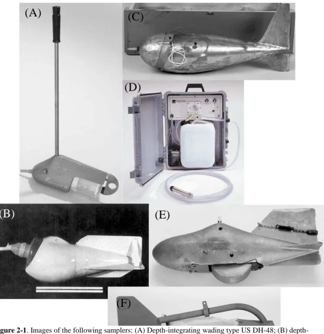
sample is collected in the field, it must be analyzed at a laboratory for any chemical species of interest. The method for determining the amount of Se in a sample varies based on the media and the species of Se of concern. The two media focused on here are water and sediments. Methods used for sampling fluvial sediments for Se analysis are highly dependent on the type of material present, ranging from large gravels to fine grain materials. It should be determined if only sediments are to be analyzed and/or if suspended sediment in the water column are to be studied as well. Also, depending on the goals of the project, a certain type of sampler should be selected based upon the size of the river or stream being sampled since each sampler has a maximum velocity and maximum flow depth or other limiting criteria for which it can be used. In general, the following types of samplers are available for use: depth-integrating, suspended-sediment samplers; point-integrating, suspended-suspended-sediment samplers; pumping samplers; bed-material samplers; and bedload samplers (Edwards & Glysson, 1999). An example of each type of sampler is shown in Figure 2-1. The last two samplers listed are for sediment alone. All other types are for sampling suspended sediments in water.

(29)

The depth-integrating DH-48 sampler is for use in smaller rivers that can be waded into safely, which is why they are lightweight (Depth-Integrating Samplers, 2009). In general, DH samplers designated with a larger number are used for larger rivers and/or those below freezing

temperatures. Point samplers can be used to collect a sample at any point underneath the surface of a stream or over a range of depth. Bed material samples are used to collect samples from

(D)

(A)

(B)

(E)

(C)

(F)

Figure 2-1. Images of the following samplers: (A) Depth-integrating wading type US DH-48; (B) depth-integrating suspended type US D-77; (C) point-depth-integrating suspended sediment US P-72; (D) pumping sampler (www.geoscientific.com); (E) bed-material US BMH-60; and (F) bedload sampler US BL-84 (Depth-Integrating Samplers, 2009 for A-C and E-F)

(30)

within the bed of a stream. Bedload samplers are made to sample the material in a stream which is in suspension above the bed and frequently maintains contact with the bed (Julien, 2010).

More than 26 different samplers are discussed in Edwards and Glysson (1999). In some cases, simple methods may be used for gathering samples in the case where the bed material is made up predominantly of coarse-grained sand to clay grain sizes. A bedload sampler would be used only to sample for material near the bed and mobilized fractions. The sediment of concern in this study is the material composing the bed must also be sampled to a depth of about 15 cm (6 in). None of the samplers discussed are suitable for extraction at this depth. Thus, plastic tubes placed vertically in the sediment of the bed or banks of the river with plastic end caps were used to collect sand and fine grained material from the surface to approximately 15 cm below the ground surface.

Numerous methods exist for collecting surface water samples for Se; however, only a few examples are discussed herein to illustrate the diversity. Zhang and Moore (1996) studied Se fractionation in Benton Lake National Wildlife Refuge, Montana and collected water samples by filtering water samples through a 0.45 µm membrane filter using a 60 mL plastic syringe that was decontaminated using an acid wash and deionized water rinse. The sample was placed into clean polyethylene bottles that had been rinsed two times by the filtered sample water (Zhang and Moore, 1996).A comprehensive study was conducted by the USGS on the collection of both surface water and sediment samples for analysis of Se. The USGS investigated four sites of the middle Green River basin that has been irrigated for over 60 years to investigate the effects of native Monaco Shale on land, water quality, and wildlife (Stephens et al., 1992). The sampling techniques used for surface water included taking grab samples of water for well-mixed low discharges and using an equal-width, depth-integrated method and a DH-48TM sampler.

(31)

Sediment samples were collected with a hand auger, composited by depth interval and placed into plastic bags or bottles. The method of analysis used for Se water samples was a hydride-generation methodology with a potassium permanganate in a hot acid solution.

The methods used for analyzing Se species in water are selective hydride generation or ion-chromatography using atomic fluorescence spectrometry or inductively coupled plasma-mass spectrometry (ICP-MS) (Maher et al., 2010). Zhang and Moore (1996) used a XAD (Alpha Products, Dankers, MA) resin separation method to determine Se species including SeO3, SeO4,

and organic Se in water as well as soluble and adsorbed fractions in sediment according to Fio and Fujii (1990). Continuous-flow hydride-generation atomic absorption spectrometry was used to determine the Se concentrations in all samples (Zhang. and Moore 1996).

Multiple procedures have been used to analyze for Se in sediments. According to Maher et al. (2010), Se speciation in sediments primarily is measured by selective extraction procedures (SEP) and X-ray absorption. For example, studying the sediments in source shales, alluvial sediments, and evaporative pond sediments near Kesterson Reservoir, Martens and Suarez (1997) used hydride generation atomic absorption measurements to test for SeO3, SeO4and

selenide that were soluble due to their extraction process. Not only were various Se species analyzed, but the analysis included organic carbon. The results of the study contend that Se concentrations and organic carbon are related in two different stages of release near Kesterson Reservoir. The first initial release of organic associated forms of Se is due to the oxidation of carbon that has accumulated because of anaerobic conditions. The second release is of refractory Se and occurs much slower due to the ecosystem change from the former Kesterson evaporation pond ecosystem (1978-1986) to a native semiarid grassland (1986-present). The results express the need to prevent refractory Se oxidation to prevent more soluble Se from entering the system.

(32)

Another study concentrating on Se speciation from source shale and testing sediments is by Kulp and Pratt (2004). Major and minor ions, total carbon, total sulfur, acid-insoluble sulfur, and total Se were tested. Kulp and Pratt (2004) also used hydride-generation atomic absorption spectrophotometry; however, they determined the concentrations of many more forms of Se including total Se, dissolved Se [SeO3 and SeO4], ligand exchangeable [SeO3 and organic Se],

base soluble [SeO3 and organic Se], elemental Se, acetic acid soluble [SeO3 and organic Se],

sulfide/selenide associated Se (-II), and residual organic Se concentrations between the detection limit of 2 mg/L and 30 mg/L Se. The study determined that the mineralogy of the sediment and what type of organic matter is associated with each rock type indicates differences in the

environmental chemistry and release of Se into the environment due to weathering (Kulp & Pratt, 2004).

Similar methods for water quality sampling have been conducted by the USGS in the Arkansas River in Colorado which have focused on measuring dissolved solids, Se, and uranium loads; unmeasured source and sinks for streamflow; and aggregating data on dissolved solids, Se and uranium loads. Ivahnenko et al. (2013) studied dissolved solids, Se, and uranium loads from June through December 2009 and from May through October 2010. Their dissolved constituents were filtered after collection through a 0.45 micrometer capsule filter and field preserved with acid to a pH of 2. Se concentrations in the Arkansas River from near Avondale to Las Animas

were found to range from 8.4 to 12.2 μg/L, exceeding the 4.6 μg/L chronic standard. Se

concentrations increased between Nepesta to La Junta and were generally higher in the tributaries. Flows from the La Junta Waste Water Treatment Plant (WWTP) had the highest median Se concentration of 18.9 μg/L. No Se concentrations at any sites exceeded the U.S.

(33)

Environmental Protection Agency primary drinking-water standards which were 50 μg/L for dissolved Se (USEPA, 2011) (Ivahnenko et al., 2013).

In the LARV, the most recent study of surface water samples collected from the Arkansas River and its tributaries for Se analysis were gathered from 2006 to 2011 using a peristaltic pump (Gates et al., 2009). Samples for total dissolved Se concentration were filtered through

disposable in-line 0.003 or 0.006 m2 0.45-µm capsule filters and placed into clean 0.12-L plastic bottles for storing dissolved metals. The location within the stream where the samples were taken was from about mid-flow depth at about the middle of the cross-section. The samples were sent to Olson Biochemistry Laboratories at South Dakota State University in Brookings, SD (USEPA certified) for analysis. The samples were analyzed via the Official Methods of Analysis of AOAC International, 17th edition, test number 996.16 Selenium in Feeds and Premixes, Fluorometric Method which can determine total dissolved Se, SeO3, and total

recoverable Se. SeO4 is estimated by subtracting the SeO3 from the total dissolved Se (Gates et

al., 2009). Gates et al. (2009) states that dissolved Se concentrations are about double the CDPHE chronic standard of 4.6 µg/L

2.5 Se Modeling

The development of computational groundwater and surface water models of Se transport begins with conceptual models of the related processes. Significant advances have been made in recent years in groundwater modeling; however, little progress has been made in the modeling of Se in surface waters.

2.5.1 Modeling Se in Groundwater (Saturated and Unsaturated)

To better understand Se cycling in groundwater in numerical modeling studies from small to large scales, several models have been developed, as summarized in Table 2-1. These models

(34)

representation of two-dimensional (2D) vertical profile flow. Recently, more finite difference models are beginning to be advanced that incorporate Se cycling in 2D to three-dimensional (3D) domains. However, a significant deficiency in these models is the lack of consideration of solute interactions such as those among C, DO, NO3 and Se.

Table 2-1. Summary of characteristics included in Se numerical modeling studies (modified from Bailey 2012) Study Mode l Dim. Satur-ated Flow Unsatur -ated Flow SeO4 SeO3 Re-dox Volatili -zation Plant Up-take Org. Matter Decay Alemi et al. 1988 1D X X Fio et al. 1991 1D X X X Alemi et al. 1991 1D X X X Liu and Narasimhan 1994 1D X X Guo et al. 1999 1D X X X X X Mirbagheri et al. 2008 1D X X X X X X X Tayfur et al. 2010 2D X X X X X X X Rajabli et al. 2013 2D X X X X X X X X Myers 2013 3D X X

The simplest Se models address 1D transport of Se species but do not include both sorption and redox reactions in saturated and un-saturated conditions (Bailey, 2012a). At least three studies have used 1D models to study sorption of SeO4 and/or SeO3 (Alemi et al., 1988; Fio

et al. 1991; Alemi et al., 1991). The first study to include the redox reactions analyzed the vertical movement of Se in groundwater by using DYNAMIX, a redox-controlled, multiple species chemical transport model beneath Kesterson reservoir (Liu and Narasimhan, 1994). Guo et al. (1999) used saturated column leaching experiments and batch adsorption tests to analyze Se sorption, volatilization, and redox reactions with parameters fitted through model calibration.

(35)

Studies that have progressed in the simulation of additional Se cycling processes in the subsurface include Mirbagheri et al. (2008), Tayfur et al. (2010), and Rajabli (2013). These studies have incorporated all major Se processes including redox reactions, sorption,

volatilization, mineralization and immobilization, and plant uptake of Se. Mirbagheri et al. (2008) simulated Se transport in an unsaturated soil column using a 1D dynamic mathematical model using a finite difference implicit method to converge on a solution. Tayfur et al. (2010) implemented a 2D finite element model that simulates Se transport in saturated and unsaturated soils. The reactions defined in Tayfur et al. (2010) are much simpler; for example, elemental Se and selenide are combined into one term. The model was tested using two datasets from

Mendota, CA. The finite-element mesh for the model testing is 616 elements and 669 nodes. The mean absolute error for the both the 1990 and 1992 dataset is 8.9% and the mean absolute error is 48.5 μg/L (Tayfur et al., 2010). The model by Rajabli et al. (2013) extends the research by Mirbagheri et al. (2008) by adding the simulation of saturated media as well as unsaturated media in a modified 3D model. The test was applied in soil columns with various fractions of silt, clay and sand. The total depth of the soil columns were 200 cm. The model was tested using data by Nasiri, et al. (2012) from the Gonbad-e-Kavous site in the Golestan province of Iran. Simulated results are supposedly in good agreement with measured values; however, at two out of eight depths the simulated results match three or fewer of the nine measured values.

Finally, Myers (2013) implements MODFLOW-2000 to simulate groundwater flow and MT3D to simulate groundwater Se transport but does so in a non-robust manner. Myers (2013) assumes that SeO4 is the primary species of Se in the groundwater in the geologic formation

simulated and does not incorporate any of the other Se processes that are included by Rajabli (2013) or Tayfur (2010).

(36)

The Se cycling relationships presented in this thesis are slightly different than those addressed in the models developed by Rajabli (2013) and Mirbagheri (2008) since they are extended to a river system. Se cycling, in general, is very similar in a surface water system as compared to a groundwater environment. However, volatilization is enhanced in the surface water environment due to the potential availability of volatilizing plants, algae, fungi, or bacteria. Reaction rates dependent on temperature can increase during the heat of the day or decrease during the winter.

2.5.2 Modeling Se in Surface Water and Sediments

Hamer et al. (2012) discuss the LAKEVIEW model of Beaver Creek which calculates concentrations of radium-226, Se, U, and TDS in a 3D water quality transport and constituent speciation model for lakes and rivers, created by SENES Consultants Limited to simulate mine waste effects. The model includes transport between the water column and sediments with three parameters: “the mass transfer coefficient between water and sediment porewater (K1), the

adsorption coefficient in the sediment for a given constituent (KD_sed), and the adsorption

coefficient of the setting solids in the water column for a given constituent (KD_Wat)” (Hamer et

al., 2012).

2.6 CSU Modeling of Salinity and Se in the Arkansas River Valley

Since 1974, several regional-scale waterlogging and salinity models of the LARV have been developed. Goff et al, (1998) created a 2D flow and solute transport model of 17.7 km of the Arkansas River. A previously calibrated solute transport model in 1973 of an 17.7 km [11-mile (mi)] reach of the Arkansas River was tested and found faulty by Konikow and Person (1985). Person and Konikow (1986) improved the previous model by incorporating salt transport throughout the unsaturated zone and refining the input data using regression

(37)

steady-state groundwater flow model of a terrace alluvial aquifer, St. Charles Mesa, south of the Arkansas River and southeast of Pueblo, CO. The model was used to evaluate the decline of the water table using various scenarios such as lining of ditches, installing dewatering wells, as well as others. All methods would lower the water table except for reduced recharge to irrigated areas and the installation of two drains enough that some groundwater wells would no longer produce water.

In 2002, a much more expansive steady-state, three-dimensional model of groundwater flow and salt transport in the USR in the LARV was published by Gates et al (2002). Later models of transient flow and salt transport in the USR were developed and applied by Burkhalter and Gates (2005, 2006) to evaluate alternative management scenarios to remediate waterlogging, salinization, non-beneficial consumptive use, and salt loading. The more refined groundwater flow model of the USR developed by Morway et al. (2013) was used in this thesis along with the reactive transport model of Bailey et al (2014) to evaluate several alternative best management practices for Se remediation.

The CSU groundwater flow model applied to the period of 1999-2007 of the USR in the LARV is a regional-scale (~104-105 ha) model of the irrigated alluvial aquifer system (Morway et al., 2013). The objectives of model development were to adequately simulate “groundwater levels, recharge to infiltration ratios, partitioning of ET originating from the unsaturated and saturated zones, and groundwater flows, among other variables” (Morway et al., 2013) under historic baseline conditions and to simulate changes in these variables under alternate BMPs over the same time period. The model builds on earlier CSU models by using a more detailed

representation of hydrologic conditions and water-budget components over a greater spatial and temporal extent as well as using larger observation data sets for calibration for the USR. To

(38)

inform the model construction and calibration, a database was built with field data collected over a period of nine years, including groundwater hydraulic head, groundwater return flow, seepage from earthen canals, actual crop evapotranspiration (ET) within the soil zone, and upflux to ET from the water table under naturally vegetated and fallow land, and estimates of ratios of water table recharge to infiltrated irrigation water. Use of the nine year data set was maximized by the following unique features implemented in the regional models:

 The time period was lengthened by six years compared to previous studies (Burkhalter

and Gates, 2005; Burkhalter and Gates, 2006) so that it includes wet, dry, and near-average hydrological conditions.

 The unsaturated-zone flow (UZF1) package (Niswonger et al., 2006) developed for

MODFLOW was incorporated and used to simulate unsaturated-zone flow processes over a regional scale.

 To create realistic spatiotemporal irrigation patterns and to preserve historical canal

diversion records, a water allocation algorithm was developed.

 For increased numerical stability during calibration (easing cell wetting and drying

problems), MODFLOW-NWT (Niswonger et al., 2011) was used.

 Spatially-varying estimates of precipitation and potential ET rates were employed in

place of uniform estimates for each region.

 Estimates of actual ET were accounted for by using highly resolved land-use and

crop-planting calibrated data classification.

 The rates and timing of seepage losses from earthen canals have been improved.  Hydraulic conductivity and specific yield values were constrained by hundreds of

(39)

The period of time simulated by the regional models is from 1999-2007 for the USR and 2002-2007 for the DSR. The grid cells have uniform areal dimensions of 250 m x 250 m in the horizontal plane which translates to a total of 15,600 active nodes in the USR. Two layers represent the alluvial aquifers of the LARV where the top layer is 5 m thick to take into account the maximum extent of deeply-rooted crops for alfalfa. The lower layer reaches from the bottom of the top layer to the impervious shale which forms the lower boundary of the modeled alluvial aquifer.

The models for each study region were calibrated using both automated and manual methods (Morway et al., 2013). The automated calibration methods used were UCODE (Poeter et al., 2005) and PEST (Doherty, 2002) which were tasked with minimizing the residual

differences between simulated and observed values of target variables. Six target variables were used in calibration. Two targets, observations of hydraulic head and groundwater return flows, were used in automated calibration. The parameters undergoing automated calibration were hydraulic conductivity and river conductance values for changing seepage. These parameters were “varied to achieve an acceptable match between model-simulated values of hydraulic head (h) and groundwater return flow to the river (QGW), and values determined from field

measurements” (Morway et al, 2013). The four targets used in manual calibration are canal seepage measurements (Martin, 2013; Shanafield et al., 2010; Susfalk et al., 2008), total actual ET calculated by the RESET model using satellite imagery (Elhaddad and Garcia, 2008), field estimates of groundwater ET (Niemann et al., 2011), and estimates of recharge to infiltration ratios (Gates et al., 2012). Using these observed data groups, manual adjustments were “made to values of canal conductance, potential ET, extinction depth, and a multiplier applied to the Ks”

(40)

Finally, engineering judgment was used to ensure that the final selected values of all calibrated parameters fell within realistic ranges (Morway et al., 2013).

The groundwater flow model for the USR was used to compute groundwater levels and flows for use in a variably-saturated reactive transport model (Bailey et al., 2014). The reactive transport model was developed by applying UZF-RT3D (Bailey et al., 2013) and accompanying Se and N reaction models (Bailey et al. 2013a) to the USR to simulate all species of dissolved Se and N in the system. Other constituents simulated are sulfur and dissolved oxygen. The Se reactions accounted for near-surface Se cycling due to agricultural processes, plant-soil

interactions, sorption, and oxidation-reduction reactions. Most redox reactions include chemical reduction of dissolved oxygen and NO3 (denitrification), nitrification and volatilization of

ammonium, volatilization of SeMet, sorption of SeO3, and oxidation-reduction of SeO4, SeO3,

elemental Se, and selenide. The chemical reactions are modeled using first-order kinetics. The

most important reaction is the “inclusion of autotrophic reduction of O2 and NO3 in the presence

of residual Se in marine shale and the associated release of SeO4into the alluvial aquifer system”

(Bailey et al., 2015). Johnsson et al. (1987) and Birkinshaw and Ewen (2000) presented

mass-balance equations that were patterned for the LARV’s N cycling module. There are seven

dissolved-phase species including O2, NH4-N, NO3-N, N2, SeO4-Se, SeO3-Se, and SeMet. There

are 16 solid-phase species. In this section, the notation for NH4-N, NO3-N, SeO4-Se, SeO3-Se

will be written as NH4, NO3, SeO4, SeO3. “UZF-RT3D solves a system of

advection-dispersion-reaction (ADR) equations for chemical species in both the dissolved phase and solid phase using the operator-split method (Yeh and Tripathi, 1989), with one ADR equation for each species” (Bailey et al., 2015). The ADR equation will be defined below for dissolved-phase Se species