Exhaust emissions from road traffic : description of driving patterns by means of simulation models

Exhaust emissions from road

traffic '- description of driving patterns

by means of simulation models

Pre-proceedings of the workshop Estimation of pollutant

emissions from transport, COST 319, on 27-28 November,

1995 at ULB, Brussels, Belgium

|»

Ulf Hammarström

Swedish National Road and

VTI särtryck 272 - 1997

Exhaust emissions from road

traffic description of driving patterns

by means of simulation models

Pre-proceedings of the workshop Estimation of pollutant

emissions from transport, COST 319, on 27 28 November,

1995 at ULB, Brussels, Belgium

Ulf Hammarström

European Cooperation in the field of Scientific and Technical Research

Estimation of pollutant

emissions from transport

Pre-proceedings of the workshop on 27-28 November

1995 at ULB - Brussels.

November 1995

f***

fr

1?

l

. .

CONTENTS

Emission Factors and Functions

Engine Maps - Available data and usage of the data, O.H. Koskinen.

Instantaneous emission maps- Available data sets and use of the data, P. Sturm and C. Study.

Cold start emission factors for passenger cars, V. Pavlidis and R. Joumard.

, Gradient influence on emission and consumption behaviour of light and heavy {duty _

vehicles, D. Hassel.

The influence of new vehicle technologies and alternative fuels on emissions factors and

functions, A.P. Green, A.P. Ivings and L. Donovan.

Life - Cycle analysis of motor fuel emissions, C.A. Lewis and M.P. Gover.

Traffic characteristics

Traffic management strategies to reduce traffic air pollution, A. Velasco.

Exhaust emissions from road traffic - description of driving patterns by means of simulation models, U. Hammarström. _

Vehicles uses derived driving cycles - a review of researches, M. André.

Mobility analysis and models of mobility, W. Hecq.

Inventorying tools

Comparison of microscale and macroscale traffic emission estimation - Tolls : DG V,

COPERT and KEMIS, Th. Zachariadis and Z. Samaras.

Bottom-up traf c emission models, E. Negrenti.

Non-Road Transport

Exhaust emission from air traffic - a review of methodologies and inventory tools, M.T._ Kalivoda.

Exhaust Emissions from Road Traf c Description of Driving Patterns by

Means of Simulation Models

U. HAMMARSTRÖM

Swedish National Road and Transport Research Institute, Olaus Magnus väg 37, S-581 95 Linköping, Sweden

Abstract

A traditional method of describing driving behaviour for vehicle exhaust emission calculations is to use measured driving cycles. There may, for example, be one typical driving cycle for urban conditions and another for rural conditions as in the US Federal Test Procedure (FTP 75). Traffic simulation models have been widely used for many years in road planning. Such models normally describe driving behaviour in some way. The description may range from a complete driving cycle to approximate data on average speed. One major advantage of simulation models is in the evaluation of future scenarios, in which case changed driving behaviour might also be included. An inventory has shown there exist many models potentially suitable for driving behaviour simulation and for calculations of vehicle exhaust emissions. The next stage of the project should result in recommendations on the choice of models and compilations of parameter values for use in the models.

Keywords

Driving behaviour; simulation models; micro and macro; inventory; urban and rural; subroutines; calibration; exhaust emissions.

1. Introduction

Why is it necessary to describe the driving cycle with simulation models? The reason is that background data are available that can be utilised more efficiently than directly measured driving cycles. Background data are defined as computerised descriptions of road network, traffic flows and vehicle fleet. A condition for using models is naturally good correlation between background data and driving cycle. Using this alternative, the driving cycle can be described for the whole of the road network for which a data description is available. In Sweden, the whole public road network is described in a data base, so that driving cycles can in principle be described with models for the complete network. Measuring driving cycles which are representative for the whole of the network is probably impracticable. The disadvantage of the model is of course that complete driving cycles reflecting the actual complex of causes in its entirety can never be simulated.

An advantage of the model is the ability to Simulate and evaluate various future scenarios. With the aid of models, new driving cycles can be simulated as a function of the future

conditions applied in the scenarios. Measured driving cycles on the other hand might in simplified terms be said to be historical as soon as they are measured.

Driving patterns can be described in two ways: continuously variable or fixed. Continuously

variable means that a model, either micro or macro, is used. Driving patterns in some form

can then be estimated as a function of road standard, traffic flow and vehicle type. The other alternative, fixed, corresponds in general to measured driving patterns, which normally means there are a fixed number of driving cycles available. Each driving cycle corresponds to one road condition class.

Most available empirical emission data have been measured in standardized test procedures with fixed driving cycles. There could for example be one driving cycle for urban and one for rural conditions. A simple and often used model for describing national exhaust emissions could then be to use empirical data from standardized test procedures directly. The advantage with such a solution would be good access to data and the disadvantage the risk for the driving cycle not being representative.

2. Driving behaviour in relation to other activities in COST 319 for estimation of vehicle exhaust emissions

A rational approach for the work on driving behaviour in COST 319 would be to start with a description of the requirements of other groups working on driving behaviour.

Engine maps refers to a mechanistic model. Contributions to the driving pattern from forces acting on the vehicle are supported directly from the model. There must be a model of the driver including:

. Handling of the gearbox 0 Handling of the accelerator . Handling of the braking system.

The handling of these variables is a function of road alignment, traffic regulation and traffic conditions.

Instantaneous exhaust emissions require a complete driving cycle or driving behaviour in matrix form. Exhaust emissions are calculated by means of a detailed emission function. Average emission factors means measured or calculated emission factors for complete driving cycles. Used driving cycles should be as representative as possible. This is the connection to the driving behaviour group.

Future vehicles will correspond to changes in vehicle performance. New driving patterns may then be estimated for different scenarios of future vehicle parameters with or without changes in driving behaviour.

Traf c management influences driving patterns, which in turn influence exhaust emissions. Tools may cover the whole range of models from micro to macro. There should be demand for tools on three different levels:

0 Macro with average speed, stops, stop duration and turning movements ' Integrating level i.e. for regional or national estimations.

If the micro alternative is chosen, this implies that there is need for driving behaviour subroutines for integration in tools or simply calibration of existing subroutines in selected tools.

If selected tools correspond to the macro alternative, work with driving behaviour should concentrate on:

o Subroutines but on another level compared to micro level

' Detailed driving patterns as a function of more approximate descriptions.

If micro models are used as tools, probably most types of traffic management measures could be described directly in tools, for example more effective signal coordination, changed speed

limits, RTI functions etc.1

If macro models are chosen as tools, the possibility for direct evaluation of traffic management measures will be significantly reduced. Nevertheless, these measures could be evaluated especially for the alternative network description with speeds and stops calculated in the model. However, most RTI functions could not be evaluated directly. This means that traffic management measures must at least to some extent be integrated into driving patterns i.e. different driving patterns for different measures.

If emissions are to be calculated for changed vehicle parameters, the most rational solution is to have models for continuously variable driving patterns inside tools.

To make calculations more "transparent", driving patterns should not be directly integrated with emission functions. One advantage of this alternative would be more flexible recalibrations for different countries.

3. Description of driving cycles

The representativity of calculated emissions depends on how the driving cycles behind them are described. The best representativity should be achieved with a high resolution of the driving cycle. An example of such a description consists of the driving sequences included in FTP 75, see Figure 1. Figure l does not include the last part of the driving cycle i.e. the repetition of the first part.

Driving speed

Figure l Urban driving cycle in FTP 75.

(km/h) 100 1 90 80 70 - 60-50 40 * 30 20 10-0 T r T T 1 I r I i! ii 1 0 500 1000

Cold start - Cold start _

first phase second phase

(transient) (stabllazed)

1 - 505 S 506 - 1371 5

In FTP 75 the description includes gearchanges as well. Possibly, the vertical road alignment should also be included to make the description as close to perfect as one could wish.

If the driving pattern is given gear changes and vertical alignment do not give anything extra to the driving pattern but are needed for the estimation of exhaust emissions.

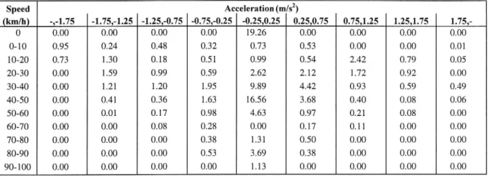
An alternative method of describing the driving cycle in Figure 1 is to use a matrix as in

Table 1.

distribution (%).

Table 1 - A presentation in matrix form of the urban driving cycle in FTP 75. Time

Speed Acceleration (m/sz)

(km/h) -,-1.75 -1.75,-1.25 -1.25, O.75 -0.75,-O.25 -O.25,0.25 0.25,0.75 O.75,1.25 1.25,1.75

1.75,-0 0.00 0.00 0.00 0.00 19.26 0.00 0.00 0.00 0.00 0 10 0.95 0.24 0.48 0.32 0.73 0.53 0.00 0.00 0.01 10 20 0.73 1.30 0.18 0.51 0.99 0.54 2.42 0.79 0.05 20-30 0.00 1.59 0.99 0.59 2.62 2.12 1.72 0.92 0.00 30 40 0.00 1.21 1.20 1.95 9.89 4.42 0.93 0.59 0.49 40-50 0.00 0.41 0.36 1.63 16.56 3.68 0.40 0.08 0.06 50-60 0.00 0.01 0.17 0.98 4.63 0.97 0.21 0.08 0.00 60-70 0.00 0.00 0.08 0.28 0.00 0.17 0.11 0.00 0.00 70-80 (100 (100 (100 (138 131 (150 (100 (100 (100 80-90 0.00 0.00 0.00 0.53 3.69 0.38 0.00 0.00 0.00 90-100 0.00

Describing driving cycles as in Table 1 requires the emissions per cell in the matrix to be independent of the immediately preceding operating conditions or that the effects of any such dependence are limited. There is of course a big advantage with the matrix form compared to the complete driving cycle description when developing typical driving cycles. The emission model should as well as the driving cycle be of matrix form.

The next level of resolution of the driving cycle in Figure 1 might be: 0 Stop duration, 20.6 sec/km

0 StOp frequency, 1.45 stops/km . Average driving speed, 40.2 km/h.

An emission model as below would be appropriate for this description of driving cycles: o Idling emissions

. Additional emissions for stops

. Average emissions as a function of speed.

When developing emission models in this case, detailed driving cycle information must be available for stops and speed separately.

The most aggregated level would be the total average speed over the whole driving cycle s 32.5 km/h.

The choice of form for describing driving pattern is determined in turn by the form of the emissions function which is to be used in parallel. Naturally, it is not sufficient to describe driving cycles with a total average speed for calculating emissions. At some point, there must be a connection between average speed and complete driving cycle.

In this case, the step from average speed to the complete description of driving cycles would be integrated in the emissions functions.

A major problem for detailed driving pattern descriptions is the way in which a small number of driving cycles could represent the infinite number of driving cycles which corresponds to reality. One sophisticated way of handling this problem is described in [l].

4. Request for information on models, subroutines and parameter values

A request, was sent out to all participants in COST 319 who had stated an interest in this matter. The result of the request was not very satisfactory since replies were only received

from Denmark, Germany, Finland, France, Spain, Switzerland and Sweden.

In most cases, the replies were more relevant to driving behaviour statistics than for models. In those cases where the replies were relevant to the request, there were no negative replies i.e. the opinion was that models for describing driving cycles could provide a good alternative or a complement to measurements. Naturally, using models as an alternative requires measurements for calibration.

5. Models

When modelling driving behaviour, the following definitions are used: 0 Micro, i.e. a complete driving cycle for each vehicle

. Macro, i.e. a simplified description as an average for groups of vehicles.

The calculation of total exhaust emissions uses a combination of direct driving behaviour data and emission functions. There is no definite boundary between micro and macro models. The closer a model comes to "macro", the more the driving behaviour data will have to be integrated into the emission functions.

Models for continuously variable driving patterns may be used as follows: 0 To calculate fixed driving patterns outside tools

0 To calculate continuously variable emission functions outside tools . Integrated inside tools.

Fixed driving patterns may be calculated by means of models or they may be measured. The number of patterns may of course be high and in practice approach the continuously variable alternative. Fixed driving patterns may be used outside or inside tools to generate emission factors.

If there is a micro model including both driving behaviour and an exhaust emission model, simplified functions for exhaust emissions may be estimated by means of the model. For example, exhaust emissions may be described as a function of speed and classified for different types of road. For each type of road, there is a special function.

5.1 Micro simulation models for free moving vehicles

The original project idea of COST 319 corresponds to complete driving cycles for individual vehicles. Such a complete driving cycle may be calculated by a specialised driving behaviour model or by a subroutine inside a vehicle exhaust emission model. Models of both types exist. A model could probably never describe a complete driving cycle in uenced by all the variables that exist in reality. With this restriction, the designation "complete driving cycles" is used here.

VETO is a computer program for calculating vehicle costs and exhaust emissions as a

function of road standard [2].

The model corresponds to "Engine maps" in COST 319.

The calculation models in VETO have been given a mechanistic design allowing great freedom in performing calculations of various properties of the road surface, different road alignments, speed limits, vehicle types and driving attitudes.

The road environment is described as follows: . Road width

0 Longitudinal gradient of the road . Lateral slope of the road surface

0 Radius of horizontal curves

0 Speed limit.

A comparatively detailed description of the vehicle is used internally in the computer program. The program works with vehicle equipages consisting either of a vehicle alone or a vehicle with trailer. The following categories of vehicle data are used in the calculations: 0 Speed regulating systems, i.e. engine, transmission and braking system

0 Masses, dimensions and moments of inertia

o Damping and springing characteristics of tyres, springs and shock absorbers

Other factors such as purchase price, vehicle age, accumulated driving distance, etc. Driving attitude is described as follows:

0 Desired speed in relation to vehicle type, road width, speed limit, horizontal radius, wearing course and road condition

. Deceleration level as a function of speed . Gearehanging as a function of engine speed o Proportion of throttle opening used.

If typical driving patterns for rural roads with traffic flows not too close to capacity are developed, this type of model should be acceptable in most cases.

This type of model is also fairly common. In Sweden, for example, there are at least three different models of this type, which are in frequent use by the automobile industry. A new and highly ambitious model of this type, consisting of modules, is also being developed in

& Sweden. There are special modules for the engine, the transmission, the driver etc. Different

members of the project will be responsible for different modules.

At least one program of this type ought to be available in most European countries. The original proposal for COST 319 was based on the existence of this type of model, the Finnish

Vehicle Simulator [3].

5.2 Micro simulation model including vehicle interactions

TRAF-NETSIM is a Fortran based program which describes in detail the operational

performance of vehicles travelling in a street network [4]. The vehicles are represented

individually and their operational performance is determined uniquely every second.

Furthermore, each vehicle is identified by a category (car, car pool, bus, truck), a type within

each category (up to 16 different vehicle types with different operational and performance characteristics) and by driver behaviour characteristics (passive, normal, aggressive).

VTI traffic simulation model [5 and 6]. The traffic simulation model describes the traffic

sequence on a two lane rural road. This is achieved by describing each individual vehicle travelling in a traffic stream along a given stretch of road. Junctions are not described in the model.

Simulation models for motorway traffic. A state of the art report on simulation models of motorway traffic is presented in reference [7].

5.3 Macro models

Macro models often work with two types of behaviour data: 0 Group 1:

- Average driving speed Number of stops Stop time

Number of turns 0 Group 2:

Driving pattern related to driving speed

Deceleration and acceleration processes related to speed at stops and turning

movements.

Group 1 data are described directly inside the model.

Speed ow functions are calibrated by means of measured data directly or by means of results from micro models. The possible additional information from macro models is that the resulting speed can be estimated as an average or per unit of time.

The number of stops and stop duration are estimated for each junction as a function of traffic regulations and conflict situations by means of special sub-models inside macro models. The number of turns at junctions could be given directly as input or estimated by means of traffic assignment models. The traffic assignment model could be a part of the macro model. Group 2 data are described and used outside the model.

Calculating exhaust emissions for estimated flow speed requires information on the driving pattern related to the flow speed. This pattern could be generated outside the model and used to calculate special emission speed functions. The functions could then be used inside the macro model and combined with speed flow functions.

If extra emissions for stops and turning movements are to be calculated inside macro models, there will be a need for extra emissions per deceleration acceleration. These extra emissions are calculated outside the model as a function of deceleration acceleration levels and speed change interval. Extra emissions per deceleration acceleration are then included in the model and are multiplied by the number of stops and turns.

TRANSYT is a computer program for calculating traffic effects and optimising signal settings [8]. Effects only include what happens at junctions, i.e. stop frequency and delay.

CONTRAM is a traffic assignment model which predict flows, queues and routes of vehicles [9].

SATURN is a traffic assignment model based on principles from TRANSYT for description of the traffic process [10].

EVA is a tool used by the Swedish National Road Administration for road planning. In this

system the "total" road network in Sweden could be described [1 l]. The system works with links and nodes.

HDM-III is a road planning model developed by the World Bank [12]. At present, a new version of HDM is being developed in a worldwide project. The new version will include subroutines for exhaust emissions.

6. Driving behaviour subroutines in simulation models For all vehicle types, there is a need for subroutines describing:

o Desired speed on a straight and level road section as a function of road width and speed limit

. Driving behaviour on horizontal curves, including: Deceleration level before the curve

Deceleration and acceleration on the curve Minimum speed on the curve

Acceleration level after the curve

' Driving behaviour on grades, which could include: Increased speed before a positive grade

- Changed desired speed, increased or decreased, on negative grades Engine power used on positive grades

0 Behaviour at junctions, including:

- Deceleration level for stops and before turns Acceleration level after stops and turns.

0 In both cases, the in uence of traffic density could be of interest. For accelerating queues, the expected acceleration level could be described as a function of queue length and vehicle type distribution.

o Gearbox handling, including:

Max engine speed when accelerating

Min engine speed at constant vehicle speed and deceleration Min engine speed at max torque

Max accepted number of gearchanges per distance driven.

The need of subroutines is in principle the same both in micro and macro models. The difference between the two alternatives is that these subroutines are more integrated in emission functions for macro models.

Speed flow functions and stop-modelling in junctions could be included into the group of driving behaviour subroutines as well.

7. Parameter values

Since 1976, speeds on straight and level road sections in urban and rural areas have been measured by VTI according to a special scheme.

Empirical data on driving behaviour on horizontal curves, in addition to driving profile and lateral position, have been measured by VTI [13].

Speed measurements have also been carried out by VTI on different types of road surfaces under different weather conditions.

A central subroutine in micro models is the description of overtaking behaviour. Two

studies have been performed, [14] and [15] for calibration of the VTI simulation model for rural roads.

8. Conclusions

The following conclusions have been formed from this preliminary study of driving behaviour described by models:

0 Both macro and micro models are available for all types of roads o Subroutines are available for most situations

. Access to certain parameter values, especially average speed on straight and horizontal road sections, could be expected to be satisfactory

0 Information on deceleration and acceleration levels for different situations is not very satisfactory

0 Information on gearshift behaviour is poor.

For regions with some kind of road data bank, micro modelling, especially for rural roads in

cases where average flow is not excessive, ought to be the best alternative in describing driving behaviour. Where the traffic flow is not excessive, the alternative with micro

simulation models for free moving vehicles could be chosen.

In the evaluation of traffic management strategies, the best alternative ought to be the possibility to use tools directly, i.e. avoiding an alternative with changes of emission factors

outside tools. If the outside tool alternative is chosen, there must be different sets of emission

factors for different traffic management strategies.

In order to continue the work on driving behaviour in COST 319, there must be well-defined

relations to the work of other subgroups. In particular, the relations to the work of the following subgroups should be described in as much detail as possible:

. Engine maps

0 Instantaneous emission . Average emission factors 0 Influence of grades on emission . Traffic management

0 Tools.

The next stage for driving behaviour models should include:

0 Tests and judgement of the suitability of different models for exhaust emission calculations . Compilation of parameter values for recommended models.

9. References

1. Joumard, R., Hickman, J., Nemerlin, J. and Hassel, D.: Modelling of emissions

and comsumption in urban areas. Deliverable N12 of the DRIVE project V1053. Bron. 1992.

2. Hammarström, U. and Karlsson B.: VETO a computer program for calculation oftransport costs as a function ofroad standard. Meddelande 501. Swedish Road and Traffic Research Institute (VTI). Linköping, 1987. 151 p + appendix.

10. 11. 12. 13. 14. 15.

Koskinen, O.: Vehicle simulator. Ministry of Transports and Communications. Helsinki. 1990 01 04. 9 p + appendix.

Rathi, A. K. and Santiago, A. J.: The TRAF NETSIM simulation program. Traffic Engineering and Control, june 1990.

Brodin, A. and Carlsson, A.: The VT1 tra c simulation model. Meddelande 321A. Swedish Road and Traffic Research Institute (VTI). Linköping, 1986. 114 p.

Gynnerstedt, G.: ICARUS Interurban Control and Road Utilisation Simulation. Swedish Model Description. Appendix B. E.C. DRIVE Contract NO.: V 1052. Deliverable 30. Royal Institute of Technology. Stockholm. 1994.

Gynnerstedt, G.: Simuleringsmodeller av motorvagstra k. State of the Art beskrivning. Royal Institute of Technology. Traffic and Transport Planning Dep. Stockholm, april 1994. 9 p + appendix.

Vincent, R. A., Mitchell, A. I. and Robertson, D. I.: User guide to TRANSYT

version 8. TRRL Laboratory Report 888. Crowthorne, 1980. 86 p.

Leonard, D. R., Gower, P. and Taylor, N. B.: CONTRAM: Structure of the Model.

Research Report 178. Transport and Road Research Laboratory. Crowthorne, 1989. 19 p + appendix.

Van Vliet, D.: SA TURN notes. The Institute for Transport Studies. The University of Leeds. Leeds, 1985. 56 p + appendix.

Calculation of ejj ects in road Analyzes. Verstion 1.1. The Swedish Road

Administration, Borlänge, 1993 11 24. 138 p.

Archondo Callao, R. and Faiz, A.: Vehicle operating cost model, version 3.0.

March, 1991. The Highway Design and Maintenance Standards Series, INUTD. The World Bank.

Lindqvist, T.: Ma'tdata för körbeteende i horisontalkurva hastighetsforlopp och korspdr (Measuring data for driving behaviour in horizontal curves driving pro le and driving track). Notat T 93. Swedish Road and Traffic Research

Institute (VTI). Linköping 1991. 46 p + appendix.

Carlsson, A.: Driving behaviour on 13 meter road width. Study ofpassings and overtakings. VTI notat T 78. The Swedish Road and Traffic Research Institute. (VTI). Linköping, 1990. 21 p.

Carlsson, A.: Driving behaviour for road width 8 9 meter. Study of overtakings. VTI notat T 95. The Swedish Road and Traffic Research Institute (VTI). Linköping, 1991. 21 p.