The Relationship Between House
Prices and the Stock Market
An investigation of the American markets
Master´s Thesis within Economics and Finance
Author: Erik Andersson
Tutor: Mikaela Backman
Pia Nilsson
Master’s Thesis in Economics and Finance
Title: The Relationship Between House Prices and the Stock Market: An inves-tigation of the American markets
Author: Erik Andersson Tutor: Mikaela Backman
Pia Nilsson Date: 2014-05-12
Subject terms: S&P 500, S&P/Case-Shiller, Granger causality, impulse response function, bivariate correlation analysis
Abstract
Stocks and houses are the two major assets on the balance sheet of American households. Changes in the two markets have a large influence on wealth and the general economy. This thesis investigates the relationship between the stock market and the house market in the U.S from 1987 to 2013. The sample period is unique since it includes two structural breaks, the dot-com bubble and the most recent financial crisis. A bivariate correlation analysis is applied to investigate the correlation and the Granger causality test, based on a vector auto-regressive model (VAR), investigates the causality between the two variables. The causality test is performed with and without GDP and interest rates as control variables. In order to investigate a potential dynamic causality, the full sample period is divided into two periods. The bivariate correlation analysis concludes that a large and positive correlation exists be-tween the two markets. All causality tests indicate a unidirectional causality running from the stock market to the house market. An impulse response function (IRF) is estimated in order to investigate the size and timing of the causality. The IRF concludes that a one percentage change in the stock market affects the house market by 0.032581 percent three years later, corresponding to a change in the value of real estates possessed by American households of 7.04 billion of dollars. The same number amounts to 47.00 billion of dollars five years later. It is concluded that the relationship has a significant influence on the wealth of American households hence a need for developing a hedging instrument which reduces the ramifica-tions from changes in the stock market is large.
Table of Contents
1
Introduction ... 4
2
Background ... 7
2.1 Accumulated Wealth of American Households ... 7
2.2 Historical Stock Market Movements ... 9
2.3 Historical House Price Movements ... 10
2.4 Comparision of the Stock Market and the House Market ... 11
3
Previous Research ... 13
3.1 Research Focusing on Correlation Analysis ... 13
3.2 Research Focusing on Causality ... 15
4
Theoretical Framework ... 18
4.1 Causal Relationship ... 18
4.1.1 Wealth Effect ... 18
4.1.2 Modern Portfolio Theory ... 19
4.1.3 Credit-Price Effect ... 20
4.2 Size and Timing of the Causality ... 21
4.3 Common Factors Influencing the House Market and the Stock Market ... 22
4.3.1 Interest Rate ... 22
4.3.2 National Income ... 24
4.4 Hypotheses ... 24
5
Data ... 26
5.1 Stock Market Index ... 26
5.2 House Price Index ... 26
6
Empirical Design ... 29
6.1 Descriptive Statistic ... 29
6.2 Bivariate Correlation Matrix Analysis ... 30
6.3 Granger Causality... 31
6.3.1 Assumptions ... 32
6.3.2 Vector Autoregressive Model ... 33
6.4 Granger Causality: Stock Market and House Market ... 34
6.5 Granger Causality Including Control Variables ... 38
6.6 Granger Causality Allowing for Structural Breaks ... 39
6.6.1 Period 1: 1987-2002 ... 40
6.6.2 Period 2: 2003-2013Q3 ... 41
6.7 Impulse Response Function ... 42
6.8 Practical Implications ... 46
7
Conclusion ... 47
7.1 Suggestion for Further Research and Improvements ... 48
References ... 50
Figures
Figure 1: Historical Developments of the Stock Market ... 9
Figure 2: Historical Developments of the House Market ... 10
Figure 3: Normalized Values of the Stock Market and the House Market ... 11
Figure 4: Impulse Response Function for House Market ... 43
Figure 5: Accumulated Impulse Response Function for House Market ... 44
Tables
Table 1: Balance Sheet of American Households 2013Q3 ... 7Table 2: Previous Studies Based on Correlation Analysis ... 14
Table 3: Previous Studies Based on Causality Tests ... 16
Table 4: Descriptive Statistics (n=107) ... 29
Table 5: Bivariate Correlation Matrix ... 30
Table 6: Testing For Stationarity 1 ... 35
Table 7: Granger Causality Test of the Stock Market and the House Market ... 37
Table 8: Testing For Stationarity 2 ... 38
Table 9: Causality Test with Control Variables ... 39
Table 10: Causality Test with Control Variables (Period 1) ... 40
1 Introduction
The stock market and the house market are two markets with different characteristics, the first one is often more volatile, more liquid and also standardized1. The housing market
on the other hand is heterogeneous, it is difficult to find two identical objects and it takes time to match buyers and sellers. Even though there exist differences, both markets offer investment opportunities and influences future wealth of households. The purpose of this thesis is to investigate the relationship between the two markets.
According to several authors, the financial crisis of 2007-2008 was the most severe since the great depression in the 1920s (Wheelock, 2010; Crotty, 2009). The stock market de-creased heavily during the crisis and wealth deteriorated for stockholders. House prices did also decrease dramatically during the same period. The crisis of 2007 began with a mortgage bubble, so obviously there existed a connection between the house market and the stock market. Was this historical event a coincident or is there a long run relationship
between the stock market and the housing market? If there is, which causes2 which?
Po-tentially there may be a dynamic relationship over time with changes in the direction of the causality. Also, when do the effect from changes occur and how large is it? This thesis aims at answering these questions. An analysis of the correlation and causality patterns will be presented. Even if the hypothesis of a relationship is rejected, there are still im-portant conclusions to draw. A weak or possible negative relationship implies that there are diversification benefits for an investor selecting to invest in both types of assets. On the other hand, a positive relationship implies that an increase (decrease) in one market is associated with an increase (decrease) in the other. Consequently, households owning both types of assets are highly exposed to changes in the two markets hence fluctuations in the stock market and the house market could have devastated ramifications for wealth. This topic is important to highlight since it can aid investors to make better investment decisions. If it is possible to identify a relationship between the two markets and also to analyze the causality, the findings can provide useful information about future changes. American households are potentially highly exposed to the two markets, hence it is nec-essary to thoroughly understand the relationship in order to restrict large fluctuations of
1 A standardization in the stock market means that it is possible to buy two identical shares.
2 In this thesis, the terms “causes” and “causality” refers to if one of the variables (markets) is granger causing
wealth. These fluctuations may also affect the health of the general economy. Moreover, it is crucial from the perspective of a policymaker to clearly understand how a potential relationship between the two markets works. It is important to be able to analyze the effects on the two markets prior to the implementation of new policies. For example, if policymakers know that house prices will cause the stock market they are also aware of that a change in a factor affecting house prices, such as the interest rate, will influence the stock market.
This study is conducted in the U.S due to several reasons. First, as a consequence of the most recent financial crisis both the house market and the stock market declined, it is interesting to investigate the relationship between the two markets prior and post of the crisis. The relationship may not be constant. Second, previous studies conducted in the U.S are available which gives an opportunity to compare the results. Third, there are sev-eral house price indices available which all defines houses and price changes in different ways. The author can therefore select how houses and price changes should be de-fined/measured. Finally, the size of the American economy is large and it has a significant impact on the world economy. The results from this study may therefore be valid in a number of other countries with a similar distribution of wealth among homeowners and stockowners.
Other studies have been investigating the relationship between the stock market and the house market in the U.S (Okunev et al, 2000; Gyourko & Keim, 1992; McMillan, 2012; Ibbotson & Siegel, 1984; Eichholtz & Hartzell, 1996; Quan & Titman, 1999; Green, 2000) however this study is unique in several aspects. The thesis investigates the relation-ship between the stock market and single family houses. The majority of previous studies includes all different types of real estates which may give another picture of the relation-ship since many corporations are real estate owners (owning warehouses, office build-ings, production plants etc.). Implying that the value of corporations (with properties as a large share of their total value) and thus its stock price, should be highly affected by changes in the value of real estates. Moreover, changes in house prices are estimated with another method. The house price index applied in this thesis is the S&P/Case-Shiller which is based on a weighted repeated sale methodology. This study is also conducted in a different time period (1987-2013) compared to previous studies. The relationship be-tween the two markets may have changed. The sample period is unique since it includes
two economic booms/recessions (The Dot-com bubble in the late 1990s and the most
re-cent financial crisis in 2007-2008), it is interesting to examine if the relationship between the two markets have remained constant around both events. Finally, this study will also investigate how fast and how much the two markets are affected by a potential causality, rather than “just” determine if a causality exist or not.
Houses can be defined in several different ways and it is vital to have a clear picture of the concept in order to interpret the results correctly. This thesis will use the very same definition of houses as the S&P/Case-Shiller price index does. The index includes single
family houses. It excludes sale prices associated with constructions, condominiums,
co-ops/apartments, multi-family dwellings and other properties that are not identified as sin-gle family houses (McGRAW Hill, 2013).
The main findings indicate a strong and positive correlation between the house market and the stock market. The Granger causality test concludes a unidirectional causality run-ning from the stock market to the house market. The impulse response function concludes that a one percentage change in the stock market affects the house market by 0.032581 percent three years later, corresponding to a change in the value of real estates possessed by American households of 7.04 billion of dollars. The same number amounts to 47.00 billion of dollars five years later.
The structure of the thesis is organized as follows, chapter 2 presents background infor-mation and a deeper motivation to why the relationship is important to understand. More-over, historical trends in the two markets are presented. Chapter 3 investigates previous studies. The theoretical framework is introduced in chapter 4. The chapter ends with hy-potheses of the relationship. Chapter 5 introduces and motivates the choice of estimators used as inputs in the thesis. Chapter 6 is entitled empirical design, it is devoted to method and statistical tests. A discussion of the results is also presented here. The thesis ends with a conclusion in chapter 7.
2 Background
This chapter starts with an investigation of the balance sheet of American households. By exam-ining the balance sheet it is possible to identify the portion of accumulated wealth consisting of stocks and houses. The same section do also present an investigation of how wealth is distrib-uted. The chapter will also investigate historical movements in the two markets and it ends with a comparison of the historical movements. The purpose of the sections is to develop an under-standing of potential structural breaks, special events and potential patterns.
2.1 Accumulated Wealth of American Households
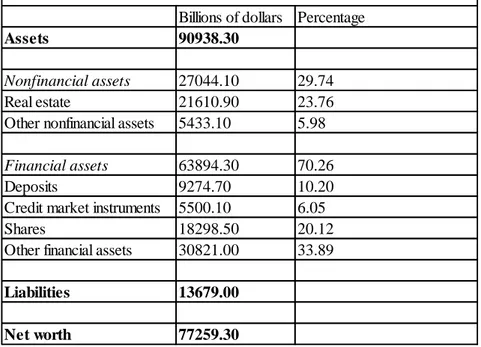
The topic is of great importance if stocks and houses are large components of the total wealth among American households. The topic is still important to investigate even if this is not the case since a change in one of the two markets might predict changes in the other. Investigating the balance sheet of American households provides information of their ex-posure to the stock market and the house market. The examination shows the percentage of total wealth consisting of stocks and houses. The original data was retrieved from the Board of Governors of the Federal Reserve System (2013). The data has been remodeled by the author, categories that are of minor interest have been consolidated. An overview of the balance sheet of American households is presented in table 1.
Table 1: Balance Sheet of American Households 2013Q3
Source: Board of Governors of the Federal Reserve System, 2013.
Billions of dollars Percentage
Assets 90938.30
Nonfinancial assets 27044.10 29.74 Real estate 21610.90 23.76 Other nonfinancial assets 5433.10 5.98 Financial assets 63894.30 70.26
Deposits 9274.70 10.20
Credit market instruments 5500.10 6.05
Shares 18298.50 20.12
Other financial assets 30821.00 33.89
Liabilities 13679.00
Net worth 77259.30
Table 1 verifies that real estates and stocks are large components, together they amount of almost 45% of the total wealth. Hence, changes in stock prices and/or house prices could have a significant impact on the wealth among American households. The severity from potential changes depends on the correlation between the two markets. A strong positive correlation increases the risk and simultaneous changes in both markets should have a large effect on total wealth. On the other hand, a low or negative correlation re-duces the risk, implying that changes only have a minor effect on total wealth.
The statistics above do not provide information of the number of households owning houses and stocks. Hypothetical, it could be the case that almost all stocks and houses are possessed by a small part of the citizens and changes in the two markets should therefore not affect the wealth of the general population. In 2010, 15.1 % of the families in the U.S had a direct ownership in publicly traded stocks. If also indirect ownership3 of stocks is included, the same number amounts to 49.9 % (Board of Governorns of the Federal Re-serve System, 2012). The rate of homeownership was 67.3 % in the U.S in 2010 (Board of Governorns of the Federal Reserve System, 2012). From this information one can con-clude that changes in the two markets should have a significant impact on the wealth of the majority of the American households.
The sections above confirm that houses and stocks are large components of the total wealth of American households. However, the topic is not only of interest for individuals owning both types of assets. It may also be of interest for individuals possessing assets in one of the two markets since movements in one of the markets might predict changes in the other. Moreover, it may also be of importance for individuals not owning any of the two assets today but who plan to be an owner in the near future. The percentage of Amer-ican households being affected by the relationship should therefore be at least as large as the numbers presented above.
3 Indirect ownership includes investments in retirement accounts, pooled investment trusts and other managed
2.2 Historical Stock Market Movements
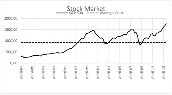
Historical movements of the S&P 5004 are investigated in order to get an understanding of trends and special events. Figure 1 is a plot of the index value of the S&P 500 from 1987Q1 to 2013Q3. Data is retrieved from Federal Reserve of Economic Data (2014-02-20).
Figure 1: Historical Developments of the Stock Market Source: Federal Reserve of Economic Data
The S&P 500 increased steadily from 1987Q1 to 1995Q1 and the volatility was fairly low. The index began to increase rapidly after 1995 and it peaked in 2000Q2 after which it decreased quickly. This period is associated with the Dot-com bubble. The volatility of the S&P 500 seems to be larger post of the crisis. The other prominent peak occurred in 2007Q1 and it is associated with the most recent financial crisis. The second peak is slightly larger than the first one with an index value of 1497 and 1476 respectively. The S&P 500 has recovered from the most recent financial crisis and its current value (2013Q3) is above the value in 2007Q1. Prior to 1997Q1, the index value has always been below the average sample value, the opposite is true Post 1997Q1, with two minor exceptions.
4 The S&P 500 is the second largest stock index in the U.S. It includes 500 stocks (Bloomberg, 2014).
0,00 500,00 1000,00 1500,00 2000,00 A p ri l-87 A p ri l-89 A p ri l-91 A p ri l-93 A p ri l-95 A p ri l-97 A p ri l-99 A p ri l-01 A p ri l-03 A p ri l-05 A p ri l-07 A p ri l-09 A p ri l-11 A p ri l-13
Stock Market
2.3 Historical House Price Movements
A similar analysis of historical house prices is also conducted. The purpose is to get an understanding of historical trends and to identify special events. Figure 2 depicts the S&P/Case-Shiller national index. Data is retrieved from S&P Dow Jones Indices (2014-02-20). The base period of the index is 2000Q1.
Figure 2: Historical Developments of the House Market Source: S&P Dow Jones Indices
The figure displays a slow and steady increase of house prices from 1987Q1 to 2000Q1 with a low volatility. Interesting to note here is that the Dot-com bubble had no negative impact on house prices. The index value began to increase rapidly around year 2000, going from a value of 100 to 190 in 6.5 years. The index peaked in 2006Q2 with a value of 190. Shortly after the peak it decreased heavily to a value of 129 in 2009Q1. The vol-atility of the S&P/Case-Shiller was low prior to the housing bubble and it increased after the crisis. In 2001Q2 the index value increased above the average value. The index level never goes below the average again in the sample period. Historical house prices can be divided into two major periods. The first period is characterized by a steady increase with a low volatility and the second period is associated with a high volatility with no clear trend. 0 20 40 60 80 100 120 140 160 180 200 A p ri l-87 A p ri l-89 A p ri l-91 A p ri l-93 A p ri l-95 A p ri l-97 A p ri l-99 A p ri l-01 A p ri l-03 A p ri l-05 A p ri l-07 A p ri l-09 A p ri l-11 A p ri l-13
House Market
2.4 Comparision of the Stock Market and the House Market
By plotting the two indices in one figure it will be possible to compare them. A graphical examination of historical movements may indicate a relationship. Moreover it will reveal whether the relationship between house prices and stock prices have remained consist-ently positive, negative or nonexistent. A period with a significant change in the relation-ship could indicate a structural break. In order to be able to compare the two indices they need to be standardized. The normalized index values5 are calculated and plotted in figure 3.Figure 3: Normalized Values of the Stock Market and the House Market Source: Federal Reserve Economic Data and S&P Dow Jones Indices. Normalized by author
The normalized index value of the S&P 500 is always above the normalized S&P/Case-Shiller index (except prior to 1991Q1). This indicates that the return from investing in the stock market in 1987Q1 and holding it during the whole sample period is larger compared to investing in houses in the same period. The figure also concludes that the S&P 500 is
5 The normalized values are calculated by dividing the current index value by the initial starting value of the
same index. 0 1 2 3 4 5 6 7 A p ri l-87 A p ri l-89 A p ri l-91 A p ri l-93 A p ri l-95 A p ri l-97 A p ri l-99 A p ri l-01 A p ri l-03 A p ri l-05 A p ri l-07 A p ri l-09 A p ri l-11 A p ri l-13
Normalized Index Values
S&P 500 Normalized S&P/Case-Shiller Normalized
more volatile than the S&P/Case-Shiller. The volatility appears to be larger for both in-dices in the second half of the sample period. A weak positive relation may be identified in figure 3 and it appears to be stronger post 2002. Both indices increased prior to the Dot-com bubble but only the S&P 500 decreased during this crisis. The indices also in-creased prior to the crisis in 2007. In contrast to the Dot-com bubble, both indices de-creased heavily after the most recent financial crisis. The decline of the stock market was larger. The figure indicates that house prices declined prior to the stock market in 2007 which could be an indicator of a unidirectional causality running from the house market to the stock market. On the other hand, only one observation indicates such causality. It could be a coincident or a unique historical event. Trend lines for both series are also plotted. They indicate an increase in both series over time. The increase is larger for the stock market.
3 Previous Research
The chapter presents previous studies of the relationship between the stock market and the house market. 3.1 examines studies of the relationship between two markets focusing on some form of correlation analysis and section 3.1 presents studies examining the causality. The two sections end with a table summarizing previous studies.
The relationship between the house market and the stock market has received much at-tention in previous research. The findings are ambiguous and explanations to this may be due to differences in statistical methods applied or in the data. Previous studies can be divided into two major categories. The first category examines the correlation between the two markets hence the methods applied are based on a correlation analysis. The other type of research investigates the relationship by using some form of causality test, these studies explains the direction of the causality.
For this thesis, it is especially interesting to consider previous studies conducted in the U.S. However studies conducted in other countries may also be of interest since they might reveal whether the results differ between countries and/or stock markets.
3.1 Research Focusing on Correlation Analysis
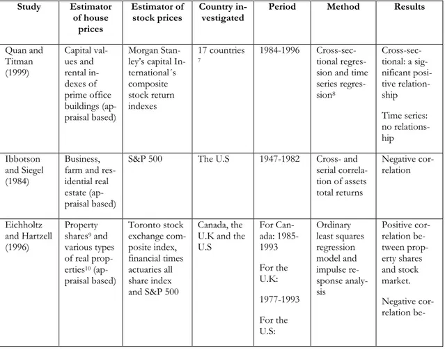
The correlation between two assets is a significant factor affecting investment decisions. The term correlation refers to how assets move in relation to one another. A high corre-lation is associated with a high level of risk. A common objective among investors is to strive after achieving the lowest possible correlation. The correlation between houses and stocks has been examined by several authors and the results are mixed. Quan and Titman (1999) conducted a time series study in 17 countries6 with data from 1984 to 1996. In addition to stock prices and real estate prices, their model also included GDP, interest rates and inflation as control variables. They found the relationship to be insignificant in 16 of the 17 countries. To investigate the issue further, the data was pooled together over a longer period of time. The cross-sectional study indicated a significant positive corre-lation. Ibbotson and Siegel (1984) examined the correlation between the returns from real estate prices in the U.S and the returns of the S&P 500 from 1947 to 1982. The correlation coefficient was found to be negative and significant (-0.06). Eichholtz and Hartzell (1996) conducted a similar study in a later time period (1978-1993). An appraisal based index
6 The Netherlands, Spain, Belgium, Germany, France, Italy, the U.K, Australia, New Zeeland, Malaysia, Japan,
(RUSSELL-NCREIF) was used as the estimator of real estate prices in the U.S and the S&P 500 represented stock market movements. The correlation was investigated with an ordinary least squares regression model. They found a negative and significant correlation coefficient (-0.09) between the S&P 500 and the RUSSELL-NCREIF index. Eichholtz and Hartzell (1996) did also investigate the correlation in Canada and the U.K, the results were similar to the regression model for the U.S. They found a significant negative cor-relation coefficient of -0.1 and -0.08 respectively. Moreover, the cor-relationship between property shares (which are similar to real estate investment trust) and the stock market on which they were listed was also investigated in the U.S. The results revealed a strong positive relationship (Eichholtz & Hartzell, 1996). Table 2 summarizes previous studies on correlation analysis.
Table 2: Previous Studies Based on Correlation Analysis
Study Estimator of house
prices
Estimator of
stock prices Country in-vestigated Period Method Results
Quan and Titman (1999) Capital val-ues and rental in-dexes of prime office buildings (ap-praisal based) Morgan Stan-ley’s capital In-ternational´s composite stock return indexes 17 countries 7 1984-1996 Cross-sec-tional regres-sion and time series regres-sion8 Cross-sec-tional: a sig-nificant posi-tive relation-ship Time series: no relations-hip Ibbotson and Siegel (1984) Business, farm and res-idential real estate (ap-praisal based)
S&P 500 The U.S 1947-1982 Cross- and serial correla-tion of assets total returns Negative cor-relation Eichholtz and Hartzell (1996) Property shares9 and various types of real prop-erties10 (ap-praisal based) Toronto stock exchange com-posite index, financial times actuaries all share index and S&P 500 Canada, the U.K and the U.S For Can-ada: 1985-1993 For the U.K: 1977-1993 For the U.S: Ordinary least squares regression model and impulse re-sponse analy-sis Positive cor-relation be-tween prop-erty shares and stock market. Negative cor-relation
7 The Netherlands, Spain, Belgium, Germany, France, Italy, the U.K, Australia, New Zeeland, Malaysia, Japan,
Sin-gapore, Hong Kong, Taiwan, Thailand, Indonesia and the U.S.
8 The models included GDP, interest rates and inflation as control variables.
9 The property shares investigated: Datastream property share index, financial actuaries property share index
and REIT of Wilshire.
10 Included in various properties are apartments, hotels, industrial, office and retail properties and sub-types
1978-1993 tween prop-erty index and stock market
3.2 Research Focusing on Causality
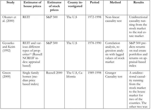
The correlation analysis do not explain the full relationship, it lacks information about the causality. A causality exists if one event causes another event. The time perspective is important, it is not possible for event B to Granger cause A if event B occurred post event A. However, event A may Granger cause event B. The causality between the stock market and the house market has received much attention in previous studies. Okunev et al. (2000) applied a nonlinear Granger causality test to investigate the causality between real estate investment trust (REIT) and the S&P 500. They concluded a unidirectional causal-ity11 running from the stock market to the real estate market during the sample period (1972-1998). Gyourko and Keim (1992) used the same type of data (S&P 500 and REIT). Their study was conducted during a shorter period of time (1978-1990) and they did also conclude a unidirectional causality running from the stock market to the real estate mar-ket. Green (2002) investigated the causality in four counties in California. Monthly data from 1989 to 1998 of the Russell 2000 stock index and houses prices from California Association of Realtors of San Francisco County, Santa Clara County, Los Angeles County and Orange County were used as estimators. The California Association of Realtors define houses as single family homes. Green (2002) concluded that house prices did not cause Russell 2000 for any of the four counties investigated. However, the Russell 2000 was found to cause house prices in two of the four counties. Hence a unidirectional causality running from the stock market to the house market existed for two of the four counties and the causality between the other two counties was independent12.
Kakes and Van Den End (2004) investigated the causality in the Netherlands from 1985 to 2002. The generalized impulse response function and the variance decomposition, es-timated from a vector autoregressive model, indicated that changes in the stock market caused changes in the house market. Except for real house prices and the AEX stock market index, the vector autoregressive model did also included real disposable income and interest rates as control variables. Ibrahim (2010) conducted a similar study in Thai-land. He concluded, by applying the Granger causality tests, an impulse response function
11 A unidirectional causality exists when variable X influences variable Y, but Y do not influence X. 12 Independence exists when none of the variables influences each other.
and variance decomposition, that the stock market caused the house market during the sample period (1995-2006).
Su et al. (2011) applied a non-linear causality test based on a threshold auto-regressive model. The sample period reached from 2000 to 2007. A unidirectional causality running from the real estate market to the stock market was evident in the U.K and the Nether-lands. The opposite, a unidirectional causality running from the stock market to the real estate market, was present in Belgium. A bilateral causality13 was discovered in Spain
and France. McMillan (2012) did also found a unidirectional causality running from the house market to the stock market. He tested the causality between the real estate market and the stock market in the U.S and the U.K using an ESTR model14. Data for real estate
prices in the U.S was estimated by the Census Bureau and the sample period reached from 1974 to 2009. The S&P 500 was the estimate of stock market movements. Table 3 sum-marizes previous studies on the causality.
Table 3: Previous Studies Based on Causality Tests
Study Estimator of
house prices Estimator of stock prices
County
in-vestigated Period Method Results
Okunev et
al. (2000) REIT S&P 500 The U.S 1972-1998 Non-linear causality test Unidirectional causality run-ning from the stock market to the real es-tate market Gyourko
and Keim (1992)
REIT and var-ious different types of prop-erties15 (Russell NCREIF in-dex: appraisal based)
S&P 500 The U.S 1978-1990 Correlation analysis, re-gression analy-sis with lagged values of stock market S&P 500 pre-dicts returns on real estate portfolios and returns on ap-praisal-based index Green
(2000) Single family homes (me-dian price based index)
Russell 2000 The U.S,
Ca-lifornia 1989-1998 Granger Causality test A unidirec-tional causal-ity running from the stock market to the house market for two of the counties. The other two was
13 A bilateral causality, or feedback, exists when the variables causes each other. 14 Exponential smooth transition model.
15 Included in various properties are apartments, hotels, industrial, office and retail properties and sub-types
found to be independent. Kakes and Van Den End (2004) Real house prices and its subcategories (Dutch NVM index: median price based)
AEX stock
index The Nether-lands 1985-2002 Generalized impulse re-sponse and variance de-composition estimated from a VAR model16 A unidirec-tional causal-ity running from the stock market to the house market Ibrahim (2010) Semi-detached houses (with/without land) and townhouses (with/without land) Stock ex-change of Thailand composite index
Thailand 1995-2006 Granger cau-sality test, im-pulse-response function and variance de-composition, based on a VAR model17 Unidirectional causality run-ning from the stock market to the house market Su et al. (2011) Not specified 18 Not speci-fied19
The U.K, the Netherlands, Belgium, France and Spain 2000-2007 Granger cau-sality test based on a threshold er-ror-correction model Mixed20 McMillan
(2012) mortgage data for proper-ties21 and
sin-gle family houses22 FT-ALL share index and S&P 500
The U.S and
the U.K 1974-2009 ESTR
23 model and an error correction model Unidirectional causality run-ning from the house market to the stock market
16 The VAR model included stock prices, real house prices, real disposable income and ten year government
bond yield.
17 The VAR model included stock prices, house prices, real output and consumer prices.
18 Not mentioned, only explain that the data was retrieved from the institute of physical planning and
infor-mation database and the DataStream database.
19 Not mentioned, only explain that the data was retrieved from the institute of physical planning and
infor-mation database and the DataStream database.
20 A unidirectional causality running from the real estate market to the stock market was eivident in the U.K
and the Netherlands. A unidirectional causality running from the stock market to the real estate market was concluded in Belgium. Feedback was discovered in Spain and France.
21 Estimates by the Nationwide are based on mortgage rates on U.K properties.
22 Estimates from the house market in the U.S are based on a media price index technique. 23 The estimated ESTR model (exponential smooth-transition model): ∆𝑌
𝑖,𝑡= (𝜃0+ 𝛼𝑖𝑌𝑖,𝑡−1+ 𝛽𝑋𝑡−1) +
(𝛽𝐸𝑆𝑇𝑅𝑋𝑡−1) ∗ (1 − exp(−𝛽𝑋𝑡−12 )) + 𝜀𝑡 Where 𝑌𝑖,𝑡 is the stock and house price series, 𝑋𝑡 is the error
4 Theoretical Framework
This chapter starts with a presentation of three theories that may explain the direction of the causality. Section 4.2 introduces information about the size and timing of a potential causality. Section 4.3 provides Information and a discussion of factors affecting both the stock market and the house market. The chapter ends with hypotheses of the relationship.
4.1 Causal Relationship
There are three major theories that may explain the causal relationship between the stock market and the house market. The first one is the wealth effect, where houses are assumed to be a consumer good. The second theory origins from modern portfolio theory and em-phasizes the need of rebalancing the portfolio if the market value of the assets included in the portfolio changes. The last theory presented is the credit-price effect.
4.1.1 Wealth Effect
The wealth effect suggests that changes in asset prices affect the net wealth of households, which in turn influences their consumption (McDowell et al. 2012). As concluded previ-ously, stocks and houses are a large share of the net wealth of households and changes in the value of both of them should influence consumption. This theory holds if houses are assumed to be a consumer good. The price of consumer goods, and thus houses, is deter-mined by demand and supply. Since it takes time to construct new houses, the supply of houses is assumed to be fixed in the short-run. An increase in demand for houses is there-fore assumed to boost house price.
The level of current consumption is determined by expectations about future wealth (Case et al. 2012). Future wealth and consumption can be explained by the life-cycle hypothesis (LCH), introduced by Brumberg and Modigliani (1954). According to the LCH, house-holds strive to maintain a constant level of consumption even though their income changes at different stages of the life. Households predict their future wealth and plan its consumption (Dornbusch et al. 2011). The choice of a household’s consumption of houses is therefore already decided. Only an unanticipated change in net wealth should affect the consumption. Hence, unexpected changes in the stock market and/or the house market influence the consumption of houses. According to the permanent income theory (PIT), the change in net wealth needs to be permanent in order to affect consumption (Dorn-busch et al. 2011). To simplify the analysis, the stock market is assumed to follow a ran-dom walk. Hence the best estimate of its future value is the present value (Gujarati &
Porter, 2009). All changes in the stock market are therefore assumed to be permanent and unanticipated. A permanent unanticipated change in the value of stocks and/or houses affects the wealth of households which in turns influences their consumption of houses. This influences the demand for houses and thus the price as well. The stock market is not affected by changes in net wealth, stocks are an investment and not a consumer good. According to the wealth effect, the level of investment is not affected by changes in net wealth. Moreover, the value of stocks is not determined by demand and supply, rather it is based on expectations about future cash flows, the risk and the discount rate associated with it (Damodaran, 2012). The wealth effect suggests a unidirectional causality running
from the stock market to the house market.
The wealth effect has been documented in the past. In the late 1990s, the rapid increase in the American stock market and the boom in the housing market (2003-2005) increased the net wealth of American households and thus their consumption increased. The oppo-site occurred when the two markets declined in 2009 and 2010 (Case et al. 2012). In practice, it is difficult to realize the profit/loss before the asset is sold. To realize a profit, and thus to be able to consume more today, households can borrow the same amount of money as the profit. Even if a household have not realized the profit they per-ceive themselves as wealthier which make them consume more today (McDowell et al. 2012). The LCH and the PIT do not account for liquidity constrains, individuals are as-sumed to be able to borrow money in times when their income is low. The theories also assume that households perfectly plan their future consumption (Dornbusch et al. 2011). These assumptions may not be realistic in practice, however they are assumed to hold in this thesis.
4.1.2 Modern Portfolio Theory
Modern portfolio theory, introduced by Markowitz (1952), focus on the expected return and the expected variance (risk) of a portfolio. The objective is to maximize the expected return, given a predetermined variance or to realize a predetermined expected return with the lowest possible variance. The theory emphasizes that the investor should evaluate the asset´s contribution to the portfolio´s overall risk and return rather than evaluating each asset individually. By looking at the overall contribution it is possible to control for a desirable level of expected return and expected variance. To achieve this, the investor
puts different weights to the assets in the portfolio depending on his/her objective (Elton et al. 2011).
If the value of stocks or houses changes, the weights in the portfolio shift. Hence the expected return and variance is affected. If the holder of the portfolio is unhappy with this new distribution he/she needs to rebalance the portfolio which is achieved by selling/pur-chasing assets. To simplify the analysis, it is assumed that the household’s portfolio con-sists of only stocks and houses and the only way to shift weights is to increase/decrease the holdings of these two assets. It is also assumed that the holder´s objective is to keep constant weights. In other words, the holder of the portfolio wants a constant risk and return distribution.
An increase in stock prices increases the value of stocks in the portfolio which disturbs the weights. To rebalance the portfolio and to keep constant weights, the portfolio man-ager must decrease the holdings of stocks and increase the holdings of houses. The de-mand for houses increases and thus the price should increase. According to the reasoning above, the two markets do affect each other. However, the house market should not affect the stock market since the price of stocks is not determined by demand. The value is based on future cash flows, the risk (discount rate) and the level of growth associated with it (Damadoran, 2012). Modern portfolio theory suggests a unidirectional causality running
from the stock market to the house market. This statement is also true if stocks are
as-sumed to follow a random walk. The best estimate of its future value is the present value, regardless of changes in demand.
4.1.3 Credit-Price Effect
A unidirectional causality running from the house market to the stock market exist if the credit-price effect is present. A large part of the majority of firms´ balance sheets consists of real estates. A change in the value of real estates should therefore have a significant impact on the value of firms and thus its stock price. Changes in the value of real estates do also influence the creditworthiness of firms. An increase in the value of the real estates increases the creditworthiness of firms and they can borrow more money and thus invest more. These investments should increase the performance of the firm, implying that cash flows and thus the stock price appreciates. Moreover, the increased demand for real es-tates should boost property prices even further (Lean, 2012; Sim & Chang, 2006;
Ka-popoulos & Siokis, 2005). The credit-price effect suggests a unidirectional causality run-ning from the real estate market to the stock market. However this study investigates the relationship between the stock market and single family houses. The study excludes other properties and the credit-price effect is therefore not expected to be present.
4.2 Size and Timing of the Causality
Many of the previous studies investigating the causality between the stock market and the house market do not provide information about the size and timing of the causality. This thesis will provide such information and the best way to gain information of the size and timing of the causality is to look at the few previous studies available investigating the issue.
Sim and Chang (2006) found a unidirectional causality running from the house market to the stock market. They used a generalized impulse response function to test how the stock market reacted to shocks in house prices and land prices in Korea. They concluded that the stock market reacts immediately to shocks in house prices and land prices. Ibrahim (2010) examined the relationship in Thailand and concluded that the stock market caused the house market. The impulse response function indicated that changes in the stock mar-ket influences the price of semi-detached houses without land immediately while the ef-fect on semi-detached houses with land and townhouses with and without land became significant after four to seven quarters.
Kakes and Van Den End (2004) studied the relationship in the Netherlands. They used a variance decomposition to prove that changes in equity prices do explain large parts of the variation in house prices twelve quarters later. An impulse response function was also estimated. The result indicated that house prices responded with an elasticity of 25 % three years after the shock in equity prices. Sutton (2002) conducted a study where the effects on the house market from shocks in the equity market were quantified. A VAR model including house prices, equity prices, national income and interest rates was esti-mated. He investigated how house prices was effected by a 10 % change in equity prices. One year after the shock, house prices changed by approximately 1 % in Canada and Ireland, the same number amounted to 0.3 % for the U.S. The effect on house prices in the U.K, the Netherlands and Australia was 1.5 %, 0.2 % and 0.7 % respectively. Three years after the shock in equity prices, house prices increased by approximately 1 % in the
U.S, Canada and Ireland. House prices in Australia and the Netherlands increased by roughly 2 %. The effect was largest in the U.K where house prices increased by approxi-mately 5 % three years after the shock.
4.3 Common Factors Influencing the House Market and the
Stock Market
The intuition behind this section is to present underlying fundamentals affecting both house prices and stock prices such as the interest rate and national income. This section will provide valuable information that is useful when developing hypotheses of the rela-tionship. Moreover, the section will also identify potential factors affecting the causality. It will be possible to investigate whether a potential causality between the stock market and the house market exist due to common underlying fundamentals or if the two markets causes each other with the effects from these fundamentals removed.
There are of course other factors also influencing the two markets. Due to limitations of space and the fact that this is a master´s thesis, it is not possible to treat all variables affecting the two markets. Inflation has been argued to influence both the stock market and the house market. However, the variable is excluded in this study. Previous studies investigating the issue (for example Kakes & Van Den End, 2004; Ibrahim, 2010) have not included the inflation either. Hence the exclusion of the inflation makes it more con-venient to compare the results. Moreover, it could be argued that some of the effect from inflation is captured in the nominal GDP, which is one of the control variables included in this thesis.
4.3.1 Interest Rate
Investments, such as stocks and houses, are highly affected by the interest rate. The risk free rate is often the benchmark for returns of more risky investments. The level of interest do also affect the present value and it is therefore important to take it into consideration before making any investment decisions. Interest rates and asset returns should have a positive relationship according to the capital asset pricing model (CAPM). According to the CAPM, investors hold only two types of assets, risky assets (such as houses and stocks) and riskless securities. The investor combines these two types of assets in order to achieve a desirable risk-return distribution. In equilibrium, the return on an efficient portfolio is determined by the market price of time and the market price of risk multiplied by the exposure to the risk (Elton et al. 2011). The CAPM describes the return on an
efficient portfolio while the Security Market Line (SML) determines the return on an individual security. The SML is based on the CAPM, equation 1 below describes the SML (Elton et al. 2011):
𝑅̅
𝑖= R
F+ β
i(R
̅
M− R
F)
(1)
𝑅̅ : Expected return on security 𝑖 𝑖
𝑅𝐹: Risk free rate
𝛽𝑖: Beta of security 𝑖
𝑅̅𝑀: Expected return on market
The first component of the equation is the risk-free rate. If the risk-free rate increases, the return on the security should also increase. Hence house prices and stocks should both be positively related to the interest rate. However, the interest rate is also a component of the discount rate which influences the present value of stocks (Damodaran, 2012). A high level of interest increases the discount rate which in turn lowers the fundamental value of the asset. Stocks and interest rates should have a negative relationship according to fun-damental stock valuation. The results from empirical studies investigating the relationship are mixed. Uddin and Alam (2007) found a significant negative relationship between interest rates and stock prices. Hissing (2004) do also support this negative relationship. Lee (1997) conclude an unstable relationship over time with a change from a significant negative relation to no relation at all. Alam and Uddin (2009) examined the relationship in 15 countries and concluded that the hypthesis of a negative relationship could not be rejected. However, for this thesis, it is of less importance to determine the nature of the relationship. More important is to determine that interest rates actually influence stock prices.
The theory of user costs of housing and rents, presented by Nakajima (2011), states that changes in the costs of owning the house should affect the price of the house. Interest payments (or opportunity cost), maintenance and repairs of the house and expectations about future prices are all parts of the user cost. The user cost of owning a house affects the demand for the house. A high user cost is associated with a low demand which in turn implies a lower price for the house. How much the interest rate affects the user costs depends on the size of the interest payments in relation to the other costs of owning the house. Interest payments (or the opportunity cost) should be a large share of the user costs for an expensive house. An increase in the interest rate is associated with an increase in
the user cost. Therefore interest rates and house prices should have a negative relation-ship, which is contradictive to the CAPM. However, empirical studies have found a sig-nificant negative relationship between interest rates and house prices (Sutton, 2002; Har-ris, 1989; Peek & Wilcox, 1991).
4.3.2 National Income
Except for the interest rate, the national income is also included as a control variable. The inclusion of control variables will provide more information about the relationship. It will be possible to determine whether the relationship exists due to common underlying fun-damentals or if a relationship also exists with these effects removed. The national income is an indicator of the state of the general economy. The national income can be measured in several ways where GDP is a common approach. The GDP influences both the house market and the stock market. It has been documented that growth in national income is positively related to changes in house prices (Sutton, 2002; Case & Shiller, 2003). En-glund and Ioannides (1997) found the one year lagged GDP growth rate to be significant for explaining house price dynamics. Sutton (2002) concluded that changes in the stock market have an impact on house prices. He explained that equity prices may forecast changes in national income which in turn affects house prices. The national income should also affect the cash flow of firms. A change in the national income affects indi-viduals income and their consumption. Changes in consumption are closely related to a firm´s revenue and cash flow. Thus national income and stock prices should be positively related. Levine and Zervos (1996) and Mohtadi and Agarwal (2001) investigated the re-lationship between national income and stock prices. Both studies concluded a significant positive relationship.
4.4 Hypotheses
Hypotheses are developed based on previous research and theories reviewed. The thesis aims at investigating three hypotheses. First, is there a relationship between the house market and the stock market in the U.S?
Previous research has investigated the correlation among the returns of the stock market and the house market. These returns were found to have a low/negative correlation. This thesis will investigate the relationship between the actual index values hence the relation-ship may be different. Figures of historical movements of the two markets indicate a
slightly positive relationship. Also the two markets react to common underlying funda-mentals in a similar way. The only indicator of a negative relationship may be the interest rate. The two markets could be negatively correlated if the interest rate has a large influ-ence on both the stock market and the house market. However, there are more factors indicating a positive relationship and these factors may have a stronger effect than the interest rates.
Hypothesis 1: There exists a positive relationship between the house market and the stock market in the U.S.
The thesis will also investigate the causality and according to both the wealth effect and modern portfolio theory, the stock market should cause the house market. It do not matter if houses are classified as a consumer good or an investment, the direction of the causality should not change. Moreover, since the value of stocks is not determined by supply and demand, stock prices should not be affected by neither the wealth effect nor the modern portfolio theory.
Hypothesis 2: There exist a unidirectional relationship running from the stock market to the house market.
The third hypothesis relates to the size and timing of a potential causality. Empirical evi-dence is weak and ambivalent. There is also a lack of theories explaining the size and timing of the causality between the stock market and the house market. The hypothesis developed origins from empirical evidence combined with authors own predictions.
Hypothesis 3: Assuming the second hypothesis is accepted, a permanent and unexpected shock in the stock market affects house prices immediately and the full effect is attained sometime after one year. The elasticity of house prices due to a shock in the stock market is between 10 % and 25 % twelve quarters after the shock.
5 Data
This chapter introduces the main inputs in the study. It starts with a motivation of why the S&P 500 is used as an estimate of stock prices followed by a thorough discussion of different tech-niques for measuring house prices. The chapter ends with a presentation and a discussion of the S&P/Case-Shiller, which will be applied as an estimate of house price movements.
5.1 Stock Market Index
This thesis investigates the relationship between the stock market and the house market at the national level in the U.S. Hence, estimators of stock market movements needs to reflect general stock market fluctuations in the whole U.S. The S&P 500 meets this crite-rion. The index contains 500 stocks from all major industries in the U.S. The purpose of the index is to measure the performance of the general economy in the U.S (Bloomberg, 2014). Moreover, the majority of previous research conducted in the U.S has used this index as an input hence it offers an opportunity to compare the findings with earlier stud-ies (Ibbotson & Siegel, 1984; Eichholtz & Hartzell, 1996; Okunev et al. 2000; Gyourko & Keim, 1992; McMillan, 2012).
Quarterly data of the S&P 500 is collected. The value reported is the average S&P 500 value for the last three months. The reported house price index value reflects market movements for the last three months. Hence the reported stock market value should not only reflect what happens in the end of the period, it should be an average for the whole three month period.
5.2 House Price Index
There are several difficulties encountered when measuring house price changes. The dif-ficulties arises mainly due to infrequent trades, non-constant quality of houses/neighbor-hoods and the fact that houses are heterogeneous. These factors make it problematic to estimate “true” house price movements. Several house price indices have been developed with different methodologies to encounter these difficulties. Extensive research has been devoted to examining the different methodologies.
Real estate investment trust (REIT) is commonly used as an estimator of real estate price changes in previous studies, see for example the work of Okunev et al. (2000) and Gyourko and Keim (1992). The index solves the problem of infrequent trades and com-parable indices can be found in several countries. However, REIT and stocks have similar characteristics. REIT is traded on the stock exchange, they offer a relatively high liquidity
and no maintenance or repairs is needed. This could be an explanation to why the REIT is closer related to movements in the stock market than other estimators of real estate prices (Eichholtz & Hartzell, 1996). Also the volatility of REIT is larger compared to real estate prices (Firstenberg et al. 1988). The index is not suitable for answering the hypoth-eses in this thesis since it includes more than single family houses. For example, shopping centers, office buildings, apartments, warehouses and hotels are often included in this index.
Other price indices applied in previous studies are based on the appraisal methodology. This methodology tends to have a smoothing effect and price inadequacies might be pre-sent (Chau et al. 2001; McAllister et al. 2003). Indices based on this methodology may therefore give a deceptive picture of price movements. The repeated sales price method-ology is another common approach for measuring house prices. It has received criticism for not taking depreciation and changes in the quality of the house/neighborhood into account. Due to this the methodology may be unreliable (Case et al. 1991). Moreover, since the index only includes repeated sales it wastes data. It may also be the case that houses sold repeatedly are not a representative sample of the population (Case & Shiller, 1987).
All indices define houses in different ways, the purpose of this thesis is to investigate the relationship between the stock market and single family houses. The index applied in this thesis must therefore only include single family houses. The index should also re-duce/avoid the shortcomings introduced above. The S&P/Case-Shiller national house
price index meets these criteria and will therefore be applied as an estimate of house price
movements. Each observation represents the sales pairs that particular month and the two preceding months. For example, the data point for March is based on sales pairs in Janu-ary, February and March (McGRAW Hill, 2013).
The S&P/Case-Shiller is based on the repeated sales price methodology and it puts four different weights to each sales pair. Firstly, all sale pairs included in the index are weighted according to price anomalies. If the price of a sale pair is far away from the statistical distribution in that particular area, the sale pair receives a lower weight hence the influence on the total index value is low. This removes some of the effects from changes in the quality of the house/neighborhood. It also eliminates potential recording errors. Secondly, the index weights according to turnover frequency. Houses that are sold
more than once during a six month period are excluded. This eliminates fraudulent trans-actions and non-arm´s-length transtrans-actions24. Thirdly, it puts different weights on each
sales pair depending on the time interval between the first and the second transaction. A longer time period is usually associated with changes in the quality of the house, transac-tions with a long time interval will therefore receive a lower weight. Lastly, the index puts a weight on all sale pairs according to the initial home value (McGRAW Hill, 2013). The major criticism of the repeated sales price methodology is reduced due to the different weighting schemes, hence the index should be reliable and track price movements well. The S&P/Case-Shiller is widely known and used, for example the office of federal
hous-ing enterprise oversight uses it (McGRAW Hill, 2013).
The problem with the waste of data is not expected to generate problems. The number of observations available at the national level is large and the exclusion of houses that are not repeated sales should therefore not have a significant impact on the national index level. Unfortunately it was not possible to find data of the number of houses sold or in-formation on the number of repeated sales included in the index. Statistics of the number of houses sold in the U.S are obviously available, but it is difficult to draw any conclu-sions from it. The S&P/Case-Shiller and other institutions do not define houses in the very same manner, hence the data can not be compared. The reader needs to be careful and have in mind that this method only includes repeated sales and may therefore not be a representative sample of the full population.
24 A non-arm´s-length transaction arises when two associates in a transaction have a relationship to each other
6 Empirical Design
This chapter includes methods, results and a discussion of the results. It starts by introducing descriptive statistics followed by a bivariate correlation matrix analysis. Section 6.3 to 6.6 is de-voted to the Granger causality test. Initially, the causality between the stock market and the house market is tested. The very same test is also applied with control variables included. Section 6.6 divides the full sample into two periods and the Granger causality is once again applied. The chapter ends with a discussion of the practical implications of the results. If nothing else is stated, all tests are performed at the 5% level of significance.
6.1 Descriptive Statistic
To get an understanding of the distribution of the variables it is helpful to investigate descriptive statistics. This examination will for example reveal whether the variables are normally distributed or not. The mean, median, maximum, minimum, current value and standard deviation for each variable is presented. Descriptive statistic for the full sample period, including 107 observations, can be seen in table 4 below.
Table 4: Descriptive Statistics (n=107) S&P 500 S&P/Case-Shiller Interest rates GDP Mean 921.23 111.51 3.60 10366.68 Median 1056.45 103.77 4.25 10283.70 Maximum 1768.67 189.93 8.54 16912.90 Minimum 255.70 62.03 0.01 4735.20 Current Value (2013Q3) 1768.67 150.92 0.03 16912.90 Standard Devi-ation 426.73 37.68 2.41 3683.46
The S&P 500 and the GDP are currently at their all-time high, indicating that the Ameri-can economy has recovered from the most recent financial crisis. The S&P/Case-Shiller is well above its mean value but the index has not recovered from the financial crisis of 2007 yet. The interest rate is close to its minimum value. The standard deviations for the variables are quite high. Some of the variables are volatile in nature (stock market). The sample period includes two economic cycles which may also contribute to the high stand-ard deviations. The standstand-ard deviation of the house market is relatively low compared to the other variables.
The mean value of the S&P 500 and the interest rate is lower than the median value, indicating that the variables are negatively skewed. The opposite is true for the S&P/Case-Shiller and the GDP. Hence the variables may not be normally distributed at their initial index values. The coefficients are still unbiased and efficient even if non normality is present. However, the t and the F tests may give misleading results. The assumption of normality is of less importance if the sample size is large (Gujarati & Porter, 2009). There are 107 observations available for each variable hence a potential violation of the normal-ity assumption should not influence the validnormal-ity of the results.
6.2 Bivariate Correlation Matrix Analysis
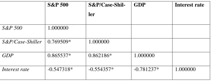
By examining the correlation between the stock market and the house market it is possible to accept or reject the hypothesis of a positive relationship. This investigation is necessary in order to get a full understanding of the relationship, the Granger causality test will not provide information regarding whether the relationship is positive or negative. A bivariate correlation matrix is therefore calculated for the S&P 500 and the S&P/Case-Shiller at their initial index values. The bivariate correlation matrix also includes GDP and interest rates at their initial index values as well. The bivariate correlation matrix is presented in table 5. Significant correlation coefficients, at the 1 % level, are marked by an asterisk.
Table 5: Bivariate Correlation Matrix S&P 500 S&P/Case-Shil-ler GDP Interest rate S&P 500 1.000000 S&P/Case-Shiller 0.769509* 1.000000 GDP 0.865537* 0.862186* 1.000000 Interest rate -0.547318* -0.554357* -0.781237* 1.000000
The S&P 500 and the S&P/Case-Shiller are strongly positively correlated and the corre-lation coefficient is significant. The two variables are also strongly positively correlated with GDP and the size of the correlation coefficients is approximately equal. The interest
rate is negatively correlated to all variables. Also here, the size of the correlation coeffi-cient between interest rates and the S&P 500 and the S&P/Case-Shiller is approximately equal. All correlation coefficients presented are significant.
The bivariate correlation matrix indicates a large and positive correlation coefficient be-tween the stock market and the house market. Figures presented in section two do also indicate a positive relationship. The two markets react to common underlying fundamen-tals in a similar way. This finding is somewhat contradictive to previous studies (Eich-holtz and Hartzell, 1996; Ibbotson and Siegel, 1984) which all discovered a low or nega-tive correlation. The contradicnega-tive result can be explained by differences in statistical methods. Instead of using a bivariate correlation matrix analysis some of the other studies have analyzed the correlation by using some form of a regression model. Also, previous studies have investigated the correlation among the returns from the two markets. This study investigates the correlation between the nominal index values. Moreover, this study is conducted in a completely different time period hence the relationship may have changed.
When it comes to concluding whether the S&P 500 and the S&P/Case-Shiller are posi-tively related or not one have to decide how the correlation should be defined. The corre-lation between the indices nominal values in the sample period is large and positive, how-ever the correlation among the returns could be different. The hypothesis of a positive relationship between the house market and the stock market is therefore accepted. Quan and Titman (1999) support this conclusion, their cross-sectional study indicated a strong positive correlation.
6.3 Granger Causality
The correlation coefficient is a standardized measure of the degree of linear association between variables. Since the correlation coefficient from the bivariate correlation matrix does not necessarily mean that one of the variables causes the others, a correlation anal-ysis is only helpful when it comes to getting an indication of the nature of the relationship (Aczel & Sounderpandian, 2009). To fully address the purpose of the thesis and to be able to accept or reject the hypothesis of a unidirectional causality running from the stock market to the house market, a causality test is included. A well-recognized test, which has also been used in previous research, is the Granger causality test. The Granger causality
test investigates the causal relationship. However, what actually causes what is a philo-sophical question. What Granger´s test of causality proves in this thesis is the predictive causality (Gujarati and Porter, 2009).
Two equations can be set up in order to demonstrate the Granger causality test: Yt = ∑ni=1αiXt−1+ ∑nj=1βjYt−j+ u1t (2)
Xt = ∑ni=1γiXt−1+ ∑nj=1δjYt−j+ u2t (3)
Where Y and X are the dependent variables. α, β, γ and δ are the estimated coefficients. The error terms, u, are assumed to be a white noise process with a zero mean, a constant variance and no serial correlation (Brooks, 2008). Equation 2 suggests that Y can be ex-plained by its own past values and lagged values of X. Similar goes for Equation 3, X can be described by its own past values and lagged values of Y. Consider Equation 2, if the coefficients for lagged values of X, as a group, are statistically different from zero and the coefficients for lagged values of Y, as a group, in Equation 3 are not statistically different from zero, a unidirectional causality running from X to Y exist. In other words, X Granger causes Y if ∑𝑛𝑖=1𝛼𝑖 ≠ 0 and ∑𝑛𝑗=1𝛿𝑗 = 0. An unidirectional causality running from Y to X can be concluded if ∑𝑛𝑗=1𝛿𝑗 ≠ 0 and ∑𝑛𝑖=1𝛼𝑖 = 0. If the coefficients for
lagged values of X and Y in both equations are statistically different from zero, as a group, a bilateral causality is indicated. On the other hand, independence can be concluded if the coefficients, as a group, are not statistically different from zero (Gujarati and Porter, 2009).
6.3.1 Assumptions
As most of the statistical tests, there are several assumptions that need to be satisfied for the results to be reliable. First, it is necessary for the time series to be stationary. This is an assumption of the standard F-test, which will be used to determine if the coefficients are statistically different from zero or not. A non-stationary process may cause a spurious regression, meaning that a statistical test may indicate two variables to have a significant statistical relationship even if their true relationship is non-existent (Brooks, 2008). A time series containing a unit root is a non-stationary process. Testing for a unit root is therefore a test of stationarity (Gujarati and Porter, 2009). The Augmented Dickey-Fuller (ADF) test and the Phillips-Perron test will be applied to evaluate whether the variables