Exchange Rate Volatility and Trade
An Empirical Analysis of Sweden’s Bilateral Trade Flows
Bachelor’s Thesis within Economics
Authors: Christoph Altvater Nils Kottmann
Tutors: Börje Johansson (Supervisor)
Bachelor’s Thesis in Economics
Title: Exchange Rate Volatility and Trade - An Empirical Analysis of Sweden’s Bilateral Trade Flows
Authors: Christoph Altvater
Nils Kottmann
Tutors: Börje Johansson (Supervisor)
Peter Warda (Deputy Supervisor)
Date: [2012-05-15]
Subject terms: Exchange Rate Volatility, Bilateral Trade Flows, GARCH
Abstract
The purpose of this paper is to test empirically how well three alternative mod-el formulations manage to explain the effect of exchange rate volatility on Sweden’s bilateral trade flows with 15 of its important trading partners. We test this through multiple time series analyses using aggregate data from the OECD, SCB, and Riksbank. None of the models is able to describe Sweden’s bilateral trade flows systematically for the period between February 1995 and October 2011. It is found that the volatility measured with the GARCH meth-od has a significant effect in nine out of the thirty investigated cases. In five cases, we find a negative relationship, while four cases display a positive effect of exchange rate volatility on bilateral trade flows. These mixed results are in line with previous research. Swedish exports seem to be more affected by ex-change rate volatility than Swedish imports. In addition, we find some evidence that the volatilities of vehicle currencies have an effect on Swedish bilateral trade flows.
Table of Contents
1
Introduction ... 1
2
Background ... 3
2.1 Exchange Rate Volatility ... 3
2.2 Previous Studies ... 5
3
Theoretical Frameworks ... 7
3.1 Hooper and Kohlhagen ... 7
3.2 De Grauwe ... 9
3.3 Broll and Eckwert ... 10
4
Data, Variables, and Descriptive Statistics ... 12
4.1 Data ... 12
4.2 Variables ... 12
4.3 Descriptive Statistics ... 16
5
Empirical Model and Analysis ... 17
6
Conclusions ... 24
6.1 Suggestions for Further Research... 24
List of References ... 26
Figures
Figure 1.1: Percentage Shares of Total Swedish Trade Volume in 2011. ... 2
Figure 2.1: Rate of Change of Exchange Rate EUR/SEK. ... 3
Figure 3.1: Hooper and Kohlhagen’s (1978) Two-Period Framework. ... 7
Figure 3.2: Effect of an Increase in Volatility on a Risk-Averse Exporter. ... 8
Figure 3.3: Effects of an Increase in the Mean-Preserving Spread of e on MU. ... 9
Figure 3.4: Broll and Eckwert’s (1999) Two-Period Framework. ... 11
Figure 4.1: Exchange Rate Volatility: GARCH EUR/SEK. ... 14
Figure 5.1: Exports: Estimated Signs for Volatility. ... 19
Figure 5.2: Imports: Estimated Signs for Volatility. ... 20
Figure 5.3: Estimated Signs for Significant Vehicle Currencies. ... 23
Figures in Appendix
Figure A 1: Volatility of USD. ... 35Figure A 2: Volatility of GBP. ... 36
Figure A 3: Volatility of CAD. ... 36
Figure A 4: Volatility of DKK. ... 36
Figure A 5: Volatility of NOK. ... 37
Figure A 6: Volatility of JPY. ... 37
Figure A 7: Volatility of CNY. ... 37
Figure A 8: Volatility of RUB. ... 38
Figure A 9: Volatility of EUR. ... 38
Tables
Table 5.1: Regression Results of Swedish Exports ... 18Table 5.2: Composition Index of Propensity to Risk ... 19
Table 5.3: Regression Results of Swedish Imports ... 21
Tables in Appendix
Table A 1: Summary of Previous Studies ... 30Table A 2: Underlying Assumptions ... 32
Table A 3: Descriptive Statistics (All Variables Except Volatility) ... 33
Table A 4: Descriptive Statistics Volatility ... 35
Table A 5: Share of Swedish Export Volumes of Goods by Industry ... 39
Table A 6: Share of Swedish Import Volumes of Goods by Industry ... 39
Table A 7: Regression Results of Swedish Exports with Vehicle Currencies40 Table A 8: Regression Results of Swedish Imports with Vehicle Currencies40
Appendix
Appendix: Previous Studies ... 30Appendix: Theoretical Framework ... 32
Appendix: Descriptive Statistics ... 33
Appendix: GARCH ... 35
1
Introduction
Sweden, as a small open economy, is heavily dependent on foreign trade. In 2010, imports of goods and services were equal to 44% of Swedish GDP while exports were equal to 50% (OECD.stat). Large parts of the economy are forced to trade with foreign firms and are therefore exposed to exchange rate risk in one form or another.
Over the course of the last century, Sweden has experimented with a variety of exchange rate regimes: Pegging the krona to gold and different currencies as well as letting it float. In this paper, we investigate the period after 1992 when the Swedish central bank, the Riksbank, was forced to abandon its peg of the Swedish krona to the European Currency Unit and had to let the krona float. The krona had not been floating for a longer period in the prior 60 years (Humpage & Ragnartz, 2006). All these regime variations raise the question what the optimal exchange rate regime for Sweden is. Should it stick with the flexible exchange rate, switch back to a fixed regime or even join the European Monetary Union? For these decisions, there are many effects of exchange rate regimes to be considered. In this thesis, we solely focus on the effects of exchange rate volatility on Sweden’s trade flows and thus weigh a small part of this discussion.
The issue of how a flexible exchange rate, and thus exchange rate volatility, influences an economy has been the topic of substantial research since the Bretton Woods system broke down in 1971. The conventional wisdom has been that exchange rate volatility influences the volumes of international trade negatively (Hooper & Kohlhagen, 1978). However, empirical studies so far have found evidence for a negative, positive, and neutral relationship between exchange rate volatility and volume of trade. This discrepancy has led to the development of other theories that explain a possible positive effect that exchange rate volatility may have on trade flows (Broll & Eckwert, 1999; De Grauwe, 1988).
The purpose of this paper is to test empirically how well alternative model formulations manage to explain the effect of exchange rate volatility on Sweden’s bilateral trade volumes measured in metric tons. We conduct a time series analysis of this relationship for the period of 1995 until 2011. The data used in this thesis are monthly national aggregates of Sweden’s bilateral trade flows over the aforementioned years. Thus, we do not focus on the aggregate world trade or sectoral data as some studies have. We report, however, on their results in the next section and discuss their relevance to our methodology later on. The trading partners we consider include the G8 countries (Canada, France, Germany, Italy, Japan, Russia, UK & USA) as well as some of Sweden’s other main trading partners. These are Belgium, China, Denmark, Finland, the Netherlands, Norway, and Spain.
These countries account for approximately 75% of Swedish trade volume. Figure 1.1 shows the percentage shares for the selected countries of the total Swedish trade volume in the year 2011 (SCB).
The empirical model we use is based on the work of De Grauwe (1988) and considers the growth of trade, the growth of real income of the trading partner, the change in the price level ratio, and the exchange rate volatility. As a proxy for exchange rate volatility we use a measure of the generalized autoregressive conditional heteroscedasticity (GARCH).
Figure 1.1: Percentage Shares of Total Swedish Trade Volume in 2011.
Data source: Statistics Sweden (SCB)
We find that none of the models is able to describe Sweden’s bilateral trade flows systemat-ically for the chosen period. Around a third of the cases display significant effects of ex-change rate volatility on trade. We find more significant cases for Swedish exports than for imports.
Our thesis is structured as follows:
Section 2 presents the background for our discussion by giving a definition for and stating the causes of exchange rate volatility. In addition, results of previous studies are presented to motivate our methodology.
In Section 3, we present three theoretical models dealing with the relationship between exchange rate volatility and trade flows. These models make different predictions about the nature of this relationship.
In the section on data, we present a proxy for exchange rate volatility and the data set that is used to test our hypotheses empirically. We conduct statistical tests to ensure that the data do not contain any patterns restricting the use of traditional statistical hypothesis testing.
In the following section, we conduct an empirical analysis of the effect of exchange rate volatility on Sweden’s bilateral trade flows. The empirical results are then analysed and compared to the predictions of the theoretical models.
In the last section, we summarise the findings from our empirical analysis and give sugges-tions for further research.
11.67 11.12 9.26 7.89 7.81 7.69 5.53 3.06 2.30 2.27 2.20 1.66 1.39 0.50 0.15 Sh ar e in %
2
Background
In order to fully understand our theoretical framework and the following discussion, we first have to establish some background knowledge of the underlying concepts discussed. We also give a basic overview of the previous research that has been conducted in this field to get a sense of what other studies have found in general and, more specifically, about the Swedish case. This also motivates the choice of the specific methodologies we use and deepens the discussion.
We deal with how exchange rate volatility develops which is important for the understanding of the problem we investigate. Moreover, the findings of this subsection motivate the choice of exchange rate volatility measure. We first present definitions for nominal and real exchange rates as well as for exchange rate volatility. Some of the various theories of the causes of exchange rate volatility are also presented. Moreover, a brief introduction on how firms can protect themselves against exchange rate risk is given.
2.1
Exchange Rate Volatility
The nominal bilateral exchange rate is generally defined as the amount of domestic currency that is needed in exchange for one unit of a foreign currency. The real exchange rate, on the other hand, looks at the prices for goods and services of one country relative to that of another country. The real exchange rate is measured by the following formula:
⁄ (2.1)
where Q is the real exchange rate, S is the nominal exchange rate, P is the domestic price level, and P* is the price level in the foreign country. Hence, the real exchange rate corrects the nominal exchange rate for differing price levels (Copeland, 2008).
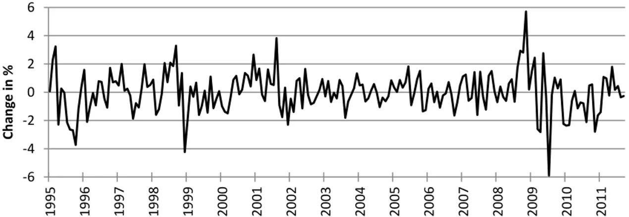
Exchange rate volatility describes the degree of fluctuations an exchange rate displays over a certain time period. The larger the range of values an exchange rate takes on within a time period, the more volatile it is. The exchange rate volatility can be derived either from the nominal or the real exchange rate (Visser, 2009). Figure 2.1 shows the monthly rate of change of the nominal exchange rate between the euro and the Swedish krona for the years from 1995 to 2011.
Figure 2.1: Rate of Change of Exchange Rate EUR/SEK.
Data Source: Riksbank -6 -4 -2 0 2 4 6 19 95 19 96 19 97 19 98 19 99 20 00 20 01 20 02 20 03 20 04 20 05 20 06 20 07 20 08 20 09 20 10 20 11 Ch an ge in %
Figure 2.1 illustrates that exchange rate volatility is not constant over time. There are periods where large fluctuations are clustered together (2009-2010) and periods where exchange rate movements exhibit only small fluctuations (2004-2008).
In the time after the collapse of the Bretton Woods system most theoretical models dealing with exchange rate determination focused on shocks to the macroeconomic fundamentals to explain exchange rate dynamics. Such macroeconomic fundamentals are, for example, the money stock, income, price level, and interest rates in the respective countries. According to these models, volatility in the exchange rate can be explained by the volatility in these macroeconomic fundamentals. An example for such a structural model that relates exchange rate movements solely on shocks to macroeconomic fundamentals is the monetary model (Copeland, 2008).
One of the most influential papers on exchange rate movements by Meese and Rogoff (1983) questions the usefulness of these structural models. They test the exchange rate forecasting ability of various structural models based mostly on macroeconomic fundamentals against several univariate time series models. Univariate time series models base their forecasts solely on information contained in past values of the exchange rate and the so-called random error term. On the other hand, structural models contain a certain number of explanatory variables that are different from lags of the dependent variable or the error term (Gujarati & Porter, 2009).
They find that a random walk performs at least as well as a structural model at forecasting out-of-sample exchange rates. This implies that the best forecast value concerning future exchange rates (St+1) is the exchange rate today (St), since the only difference between the
two levels is a random error term (ut+1):
(2.2)
These findings have shifted the focus of researchers on other effects than shocks to the fundamentals that influence the foreign exchange market, and hence the volatility in bilateral exchange rates.
Several factors explain why exchange rate volatility exceeds the volatility that can be attributed to fluctuations in the fundamentals. For example, local currency pricing is a source of incomplete exchange rate volatility pass-through where exchange rate changes are not completely passed down to consumers and thus cause excess volatility (Devereux & Engel, 2002). Another factor is the existence of noise traders, i.e. traders who have imperfect information about the fundamentals determining the exchange rate, because they display an irrational volatility (Jeanne & Rose, 2002). The degree of confidence in the capabilities of the central bank also influences the magnitude of exchange rate volatility. A high degree of confidence, all else equal, leads to small fluctuations whereas large fluctuations can be caused by a low degree of confidence (Dunn Jr. & Mutti, 2004). This makes predicting exchange rates problematic.
International trading firms can protect themselves against this uncertainty through hedging. The availability of hedging further complicates the study of the effects of exchange rate volatility. If firms use hedging intensively enough, it offers a possible explanation for insignificant effects of volatility in exchange rates on trade flows. We shortly present two of the main financial derivatives that can be used to hedge (Friberg, 2008).
According to Friberg (2008), the most frequently used financial derivative to hedge against exchange rate uncertainty is forward contracting. A forward contract is a legal contract that
forces a party to buy or sell a specific currency at a certain point in time at a specific rate. Thus, exchange rate movements have no effect on the profit from the hedged contract. Another way to hedge is to buy an option. When buying an option, an economic agent buys the right to buy or sell a particular currency at the price that is specified in the contract. This price is called the strike price. When deciding whether to execute the option or not, the spot price at the option’s maturity is compared to the strike price specified in the contract.
Even though it is possible to hedge against exchange rate volatility, it is not possible for all economic agents to secure all their trade operations due to the limited variations of hedging contracts available. Moreover, empirical evidence suggests that exchange rate volatility has a measurable effect in many cases. However, previous research has reached mixed conclu-sions about the nature of this effect (cf. Bahmani-Oskooee & Hegerty, 2007; De Grauwe, 1988; De Vita & Abbott, 2004).
2.2
Previous Studies
Since the collapse of the Bretton Woods system, the issue of how exchange rate volatility affects the volume of international trade has been intensely researched. However, even with this vast research, there is no consensus on this relationship in either theoretical or empirical studies to be found. Some explanations for this are unsuitable empirical methods and the availability of hedging (Bini-Smaghi, 1991; Bahmani-Oskooee & Hajilee, 2011). We explore these and more in the review of previous literature and deal with the theoretical models of the relationship in the next section.
Since there is a vast amount of prior research to be considered, we focus this section on the findings for Sweden as well as some major studies. We have summarised these studies in Table A 1 which can be found in Appendix: Previous Studies.
There is no consensus in the literature on the correct volatility measure to use. Variations on standard deviation, which measures the volatility for a certain number of periods in the past, are widely used. However, autoregressive conditional heteroscedasticity (ARCH) methods have become more popular in recent years. They are also found to be the most efficient measure by some comparative studies (cf. Seabra, 1995; West & Cho, 1995). Studies usually use quite similar regression models. For the most part, they are based on either simple supply and demand models or gravity models but vary on which explanatory variables to include (Bini-Smaghi, 1991; Dell'Ariccia, 1999).
Studies have also been divided on the issue of whether to measure the volatility of the nominal or the real exchange rate. The results of using nominal or real exchange rates do not vary greatly from one another because both move closely together (Qian & Varangis, 1994; Thursby & Thursby, 1987).
Many studies investigating Sweden find a negative relationship between exchange rate volatility and trade. Abrams (1980), Thursby and Thursby (1987), as well as Brada and Méndez (1988) find a negative relationship for Sweden’s export value. Brada and Méndez (1988) also conclude that a floating exchange rate regime affects overall trade positively. Kenen and Rodrik (1986) find a negative relationship for aggregated import volumes of the major industrial countries. However, for Sweden their results are not significant. Arize (1995) finds a negative effect on Swedish aggregate export volumes in the short-run and
the long-run. Dell’Ariccia (1999) finds the same when pooling the data for the EU15 and Switzerland.
On the sectoral level, Lee (1999) investigates the effect of exchange rate volatility on U.S. imports of manufacturing, durable, and non-durable goods from the G-7 and some smaller economies, including Sweden. He also finds evidence for a negative relationship of volatility with the volume of imports.
Empirical studies do not only find negative relationships but also frequently positive ones for Sweden. Qian and Varangis (1994) examine aggregate export volumes and use ARCH to measure volatility. They find that volatility positively affects Swedish trade, while it negatively affects other economies (Canada & USA) over the period 1974-1990. They propose that this could be because Swedish exports were mostly priced in the domestic currency during this time. This transfers all exchange rate risks to importers of Swedish goods, which in turn can pass it on to consumers. During the peg of the Swedish krona, it was devalued three times, which led to increased exports. However, even accounting for this, exports were still positively affected by volatility. They note that exchange rate volatility may be more of a problem for developing countries exporting primary commodities since these are generally priced in U.S. dollar or pound sterling. Arize (1998) analyses the aggregate import volumes of several European nations and finds that Swedish imports are positively affected by exchange rate volatility over the period 1973-1995. A thesis by Carlsson (2003) also finds evidence for a positive influence on Sweden’s bilateral trade flows over the period 1993-2000.
De Vita and Abbott (2004) find a positive effect on UK exports to Sweden, while their sectoral analysis only yields significant results for the exports of services from the UK. These results, however, are based on short-term risk, which is easier to hedge against than long-term risk. When applying a long-term measure they find a significant negative effect of volatility on UK exports to Sweden. These results are somewhat complemented by Bahmani-Oskooee and Hajilee (2011). They analyse the effect of volatility on imports and exports of 87 industries between the U.S. and Sweden, and their results also vary depending on whether they investigate the short or the long-run effect. In the short-run, volatility has a significant effect on Swedish imports in about two-thirds of the industries. These are positive in some industries and negative in others. In the long-run, the effect of volatility is less pronounced and in only about one-fifth of the cases significant. Whether the relationship is positive or negative still depends on the industry. They find no specific characteristics determining whether an industry reacts positively or negatively to volatility. The effect on Sweden’s exports is similar.
These differing results serve to frame the discussion going forward. The debate over how and if exchange rate volatility affects international trade flows is obviously far from settled and makes the results we expect to obtain from our own empirical analysis unpredictable. This discussion also extends to the underlying theories, which we deal with in the next sec-tion.
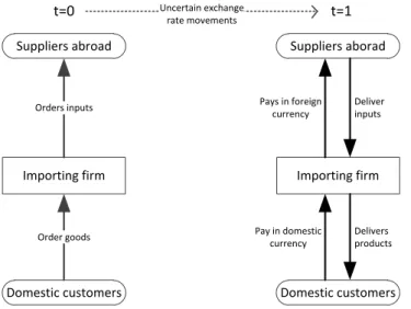
t=0 Importing firm Suppliers abroad Orders inputs Domestic customers Order goods Uncertain exchange rate movements t=1 Importing firm Suppliers aborad Domestic customers Pays in foreign currency Deliver inputs Pay in domestic currency Delivers products
Figure 3.1: Hooper and Kohlhagen’s (1978) Two-Period
Framework.
3
Theoretical Frameworks
Exchange rate volatility is not included in standard trade theory. Hence, we have to consult models that specifically investigate this relationship (Krugman & Obstfeld, 2009). We first present one of the earlier and perhaps most widely used theoretical models, which was developed by Hooper and Kohlhagen (1978). It predicts a negative relationship between exchange rate risk and trade for all risk-averse firms. We include it because it presents the classical view of the issue of exchange rate risk and because it lays some foundation for the second model we present. We use a slightly modified version of De Grauwe’s (1988) model for our empirical analysis and therefore present its theoretical foundation here. This model can be used to explain both a positive and a negative relationship, depending on the degree of risk-aversion of firms. Lastly, we present Broll and Eckwert’s (1999) model, which predicts a positive relationship to round off the discussion. A summary of the underlying assumptions of the three models can be found in Appendix: Theoretical Framework (Table A 2).
3.1
Hooper and Kohlhagen
Hooper and Kohlhagen (1978) have developed a widely used theoretical model concerned with the effect of exchange rate uncertainty on trade flows in the years after the Bretton Woods system was abolished.
This theoretical model predicts a negative relationship between exchange rate volatility and the volume of trade when economic agents are risk-averse. The model also discusses the effect on prices, which we do not discuss extensively.
The model is set in a two-period framework. We summarise this framework in Figure 3.1. In the first period (t=0), the importing firm receives orders from its domestic customers. At this time, the importing firm orders the necessary inputs from abroad to meet this demand. In the second period (t=1), the importing firm pays its suppliers abroad in the foreign currency. It also delivers its products to the domestic customers who pay immediately in the domestic currency. At t=0, it is uncertain how much the importing firm will have to pay for the inputs in its domestic currency since they are assumed to be priced in the foreign currency. It is uncertain because the exchange rate at t=1 is unknown at t=0. One of the assumptions is
that all contracts are priced either in the domestic or the trading partner’s currency. Thus, no vehicle currency, i.e. a third currency to price contracts in, is used.
The equilibrium level of import demand and export supply is affected, among other things, by the degree of exchange rate volatility.
The import demand and export supply functions are first derived for individual firms from their utility functions and then
aggregated. The utility of an importer or exporter depends on the expected profits and on the variance of these profits, which itself is affected by the degree of exchange rate volatility. Whether the variance of profits is negatively or positively related with utility depends on the attitude towards risk of the importer or exporter.
There are three different attitudes towards risk. An economic agent can either be risk-averse, risk-neutral, or risk-loving. Risk-aversion implies that the economic agent undertakes the least risky action among several options that yield the same expected profit. Least risky refers to the action with the lowest variance in possible outcomes. Risk-neutral agents are indifferent between several options with the same expected outcome but different degrees of risk. Hence, they do not consider risk when making decisions. Risk-loving agents, on the other hand, prefer large variances in the expected outcomes. For risk-averse importers, the variance of profits has a negative effect on their utility. The variance of profits is positively associated with utility if the importers are risk-loving, while it has no effect in the case of risk-neutrality (Machina & Rothschild, 2006).
The profit function of an importer includes revenue, production costs, and a separate cost term that captures all the costs that are associated with foreign exchange. This cost term is affected by the currency the contract is priced in and by the relative amount of contracts that is hedged.
Both the importer and the exporter face uncertainty because future movements in the exchange rate are unknown. At the same time, not all trading activity is invoiced in their respective domestic currency, nor is all trading activity in the foreign currency hedged against fluctuations in the exchange rate.
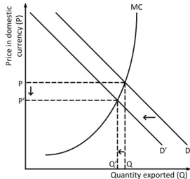
An increase in exchange rate volatility causes an increase in the variance of profits. An increase in the variance of profits leads to a decrease in the utility gained from trade if both importers and exporters are risk-averse. Therefore, demand for imports shifts to the left. Figure 3.2 shows the effect of an increase in exchange rate volatility on a risk-averse exporter. All else equal, an increase in the exchange rate volatility leads to a shift to the left of the aggregate demand schedule for imports. This shift leads to a decrease in the quantity
exported and eventually a fall in price.
For risk-loving trading partners the opposite is true. An increase in the exchange rate volatility shifts import demand to the right. The equilibrium level of trade is not affected in the case of risk-neutral trading partners: No shift occurs.
The attitude towards risk of the importers and exporters are crucial for the direction of the effect of exchange rate volatility on the equilibrium level of trade. If both parties are risk-averse there is a negative relationship between the two variables. In the case that both importers and exporters are characterized by having a neutral attitude towards risk there is no effect on the trade volume due to a change in the degree of exchange rate volatility. A risk-loving attitude
MC D’ D P ri ce in d o m es ti c cu rr en cy ( P ) Quantity exported (Q) Q Q’ P P’
Figure 3.2: Effect of an Increase in Volatility on
a Risk-Averse Exporter. Source: Hooper & Kohlhagen (1978)
causes a positive relationship between the two variables in question.
3.2
De Grauwe
De Grauwe (1988) comes to a less clear-cut conclusion than Hooper and Kohlhagen (1978) do. He also finds that whether exchange rate volatility affects trade positively or negatively depends on the attitude towards risk of the economic agents. However, he shows that a very risk-averse individual would increase exports with an increase in exchange rate volatility, while a less risk-averse individual would do the opposite.
The export volume is determined by maximising the utility function, which is only dependent on the income the exporter earns from his or her trade activities. Due to the fact that the exporter is assumed to be risk-averse the utility function has a concave shape. In this model, a firm’s profit depends on the amounts it produces for the domestic and the foreign market. The producer has to decide what amount of resources to use in these two sectors. The only element of risk in this model is the exchange rate, which determines the profit a firm receives from its exports. The utility is maximised with respect to the quantity produced that will be exported.
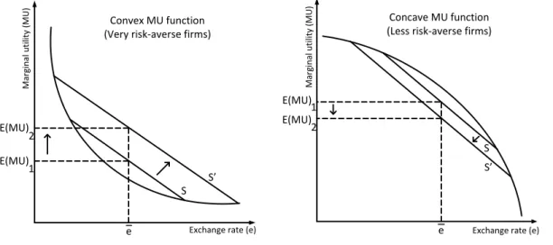
In his analysis, he arrives at a marginal utility (MU) function of the exports depending on the exchange rate (e). Whether this marginal utility function is concave or convex depends on the degree of risk-aversion of the trading firms. Very risk-averse firms have a convex marginal utility function, whereas less risk-averse firms have a concave marginal utility function. He then analyses the effects of a mean-preserving increase in the spread of the exchange rate (S) on expected marginal utilities (E(MU)). That is, how a higher volatility with the same mean value of the exchange rate ( ̅) affects the expected marginal utility of exports. Whether a mean-preserving increase in the spread of the exchange rate increases the expected marginal utility of exports or not, depends on the shape of this marginal utility curve: whether it is convex (increase in exports with increase in volatility) or concave (decrease in exports with increase in volatility). Figure 3.3 shows for both cases of risk- aversion: e E(MU) E(MU) 1 2 M ar gi n al u ti lit y (M U )
Exchange rate (e)
Convex MU function (Very risk-averse firms)
S S’ e E(MU) E(MU) 1 2 Concave MU function (Less risk-averse firms)
M ar gi n al u ti lit y (M U )
Exchange rate (e)
S S’
Figure 3.3: Effects of an Increase in the Mean-Preserving Spread of e on MU. Source: De Grauwe (1988)
De Grauwe finds that the expected marginal utility of export revenues rises with an increase in exchange rate risk for very risk-averse producers, while the opposite is true for less risk-averse producers.
This is because income and substitution effects lead to different results for very risk-averse and less risk-averse individuals. The substitution effect describes the reduction in risky activity due to an increase in its riskiness. The income effect has the opposite consequences. The income effect describes the increase in risky activity to compensate for the reduction in total expected utility. The total expected utility of exports decreases with an increase in risk and in order to compensate for that, firms allocate more resources to the export sector, and thus export more goods. Firms would choose to export less if the substitution effect is dominant over the income effect and more if the income effect is the dominant one. An increase in exchange rate risk (increased spread of export revenue around the mean) lowers total expected utility but may in fact increase the expected marginal utility. Thus, although all firms are made worse off by the presence of exchange rate risk, some may choose to export more because of it.
He reasons that this is because very risk-averse individuals are concerned about the worst possible outcome. In order to avoid the possibility of a radical decline in revenues they export more. On the other hand, less risk-averse individuals are not as concerned with extreme outcomes and choose to export less.
De Grauwe’s (1988) model presents explanations for both a positive and a negative rela-tionship between exchange rate volatility and trade flows. The sign of this relarela-tionship de-pends on the degree of risk-aversion of the trading firms. On the other hand, Broll and Eckwert (1999) derive a model that predicts a positive relationship that is not dependent on the degree of risk-aversion.
3.3
Broll and Eckwert
Broll and Eckwert’s (1999) model consists of a two-period framework of a price-taking, risk-averse firm. A price-taking firm is too small to affect price levels and is able to sell all of its products at the equilibrium price level determined by the market for its goods. Hence, the only variable these firms can vary in order to maximize their profits is the quantity produced. The profits of a single firm are positively related to total revenues but decrease with total costs, which are assumed to be solely dependent on the quantity produced.
At t=0 all prices of goods are known, however, the exchange rate at t=1 is unknown. At t=0 the firm has to decide how much to produce, but it has time until t=1 to decide whether to sell the produced goods in the domestic market or abroad.
Since the domestic price at t=1 is known at t=0, there is no uncertainty about the profits realized when the firm sells all goods produced in the domestic market. The profits earned when the production is sold entirely in the domestic market can be considered the minimum profit level of the firm. The firm will not choose to export if the foreign price expressed in domestic currency at t=1 is less favourable than the domestic price.
If the foreign price of the goods expressed in the domestic currency rises above the domestic price due to exchange rate fluctuations, the firm will capture the higher price by exporting all its goods. By being able to choose between exporting and selling in the domestic market, the firm can optimize its profits compared to only being able to follow
one strategy. A firm that only exports faces randomly determined prices for its goods due to random exchange rate fluctuations. On the other hand, a firm that only operates in the domestic market can only realize the domestic price.
We summarise this framework in Figure 3.4. It shows the decisions the firm has to make as well as the available information about prices for the two periods.
t=0 Firm Uncertain exchange rate movements t=1 Firm How much to produce Decides · Domestic price at t=1
· Foreign price in foreign currency at t=1
· Domestic price at t=1
· Exchange rate at t=1
· Foreign price in domestic currency at t=1
Knows Knows
Export
Sell in domestic market
Domestic price < foreign price in domestic currency
Domestic price > foreign price in domestic currency
Figure 3.4: Broll and Eckwert’s (1999) Two-Period Framework.
In short, Broll and Eckwert (1999) treat the possibility to export as a call option. The domestic price is the strike price, and, depending on the realized exchange rate, the option to export is exercised or not. Thus, the firm either exports all its goods at t=1 or none. Higher exchange rate volatility increases the value of this option. This is because with higher volatility it is possible to realize higher returns. Yet, due to the nature of the option, the minimum the firm can earn is the domestic price of its goods.
This model, although not applicable to all industries, can be argued to be reasonable for some industries. The authors mention the agricultural sector and sectors that have reached their capacity limit as examples for this.
In conclusion, these theoretical works make different predictions about the influence of exchange rate volatility. This variety is useful for our analysis later on.
Hooper and Kohlhagen (1978) predict an unconditional negative relationship between exchange rate volatility and trade volume as long as economic agents display risk-aversion. De Grauwe (1988) also concludes that with moderately risk-averse economic agents trade flows are negatively affected by increased exchange rate volatility. He differs in that he predicts a positive effect for a very high degree of risk-aversion. Broll and Eckwert (1999) go even further and predict a positive relationship regardless of the degree of risk-aversion, although they admit that their model may not be an appropriate approximation for all industries.
This leads us back to our original question: Which of these models has the strongest support from the empirical data in the case of Sweden? This is what we test and discuss in the following sections. First, we present how we transform the data used. Then we try to find possible explanations for our results and take the argumentations of these theories into account.
4
Data, Variables, and Descriptive Statistics
In this section, we present the data set that is used in the multiple time series analyses of Section 5, how we transform it, and any irregularities in the data. We discuss how we construct the variables that are used in our empirical model. These are exchange rate volatility, trade volume, price level ratio, and output. We deal with the various advantages and disadvantages of the proxies used and justify our usage of them. First, we discuss the data set and the method of calculating the variables, and we end this section with a short discussion of the descriptive statistics.
4.1
Data
We use monthly data for the period from February 1995 to October 2011, which gives us 201 observations per time series. The period covered is different for China and Belgium because not all data are available for the missing time periods. Belgium is covered from January 1998 until October 2011 (165 observations), whereas China is covered from February 1995 until November 2003 (124 observations).
We use natural logarithms on some of our variables to obtain elasticities directly from our estimated regression coefficients. In order to avoid non-stationarity for all variables, we take the first difference for all our variables except for our volatility measure. This is necessary because non-stationarity can lead to spurious regressions (Gujarati & Porter, 2009). The first difference is also taken from the natural logarithms to approximate percentage changes. If extreme outliers are identified that might negatively affect our regressions, we bind their values to the 1st and 99th percentile respectively.
The monthly average bilateral exchange rates from which we calculate the exchange rate volatility are obtained from the database of the Riksbank. Statistics Sweden (SCB) supplies the data necessary for the calculation of the price level ratio and the trade volume. The OECD provides us with the data for the output variable. The next subsection shows how we transform these data sets to construct the variables. We begin with the dependent vari-able: trade volume.
4.2
Variables
Trade Volume
In order to measure the impact of exchange rate volatility on bilateral trade volumes, we need to quantify the Swedish exports (EX) to and imports (IM) from the various countries under investigation. In this paper we utilise, the volumes of exports and imports, measured in metric tons. Our data for exports and imports only include the volume of goods traded and disregard the bilateral trade in services. Later, this narrows down our analysis and has to be kept in mind. We do not use the absolute volume but rather the growth in the volume traded ( ).
This is accomplished by taking the first difference of the natural logarithm of the exports and imports respectively:
Exchange Rate Volatility
Our measure of volatility of the exchange rate is based on the volatility in the previous period, the error term in the previous period as well as the average variance (Engle, 2001). We use a univariate time series method to create a proxy for the exchange rate volatility in line with Meese and Rogoff (1983). One of these time series methods that has become very popular when modelling the volatility of financial data including exchange rate movements is the so-called generalized autoregressive conditional heteroscedasticity (GARCH) method. Seabra (1995) finds that GARCH outperforms other available volatility measures. Therefore, we only use GARCH to measure volatility. The GARCH method is a generalised form of the autoregressive conditional heteroscedasticity (ARCH) method developed by Engle (1982). The idea behind the ARCH method is that the conditional variance of, for example, financial series is not constant over time. Volatility is clustered which means that high volatility is most likely followed by high volatility. Hence, the conditional variance is not homoscedastic, but heteroscedastic.
In the case of a univariate autoregressive moving average [ARMA(1,1)] model of the exchange rate, is a function of the first lag of the dependent variable [AR(1)] and
the first lag of the error term [MA(1)], as presented in Equation 4.2:
(4.2)
where is the constant term, θ and ζ are the ARMA coefficients, and εt is the error term.
The GARCH (p,q) formula for this model is:
∑ ∑ (4.3) where
and α0 is the constant term, is the parameter coefficient of the ARCH term , and
is the parameter coefficient of the GARCH term . The order of the ARCH is equal to p, and the order of the GARCH is equal to q. The ARCH term captures the influence of the previous error terms, and the GARCH term captures the influence of the previous volatility values. In order to avoid spurious regressions the GARCH condition of stationarity needs to be fulfilled:
∑
∑
(4.4)
The appropriate order of the GARCH is decided for each exchange rate individually with the help of the Akaike Information Criterion (AIC) (Bollerslevs, 1986).
As mentioned earlier, it is possible to calculate the exchange rate volatility from the nominal or the real exchange rate. In this paper, we use the nominal exchange rate since we
want to ensure to solely capture exchange rate fluctuations and not price level fluctuations (Bini-Smaghi, 1991).
The exact methodology of calculating the volatility from the average monthly exchange rate with the help of the GARCH method can be found in Appendix: GARCH.
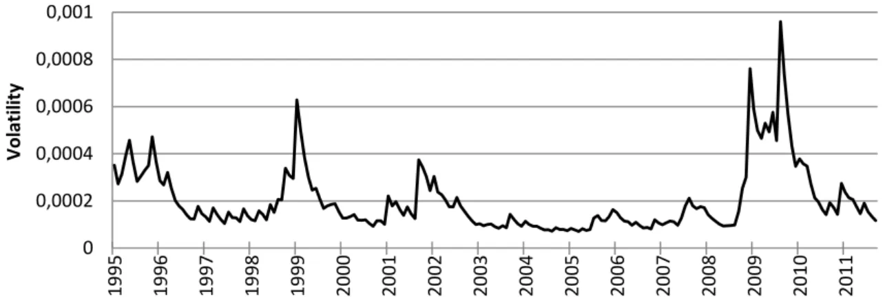
The procedure is applied to the change in the exchange rate between the euro and the Swedish krona, where the monthly results obtained are presented in Figure 4.1. Comparing this to Figure 2.1, we reach the same conclusions: Periods of high volatility (2009-2010) as well as periods of low volatility (2004-2008) are clustered together.
Figure 4.1: Exchange Rate Volatility: GARCH EUR/SEK.
Data source: Riksbank
The graphs for all other volatilities derived from the various exchange rates can be found in Appendix: GARCH (figures A 1-9).
In the case of the Russian rouble, we have to transform the data due to a drastic redenomination in January 1998. In order to avoid extreme outliers, which might have a strong impact on our regression, we bound the extreme values of the change in exchange rate to the values of the 1st and 99th percentile respectively.
We adjust the GARCH estimates of the Chinese yuan and the Norwegian krona in order to ensure that the necessary constraints for Equation 4.3 hold. Therefore, integrated generalized autoregressive conditional heteroscedasticity (IGARCH) is used instead of ordinary GARCH to make sure that the sum of the coefficient parameters are not larger than one, which is in line with Nelson (1990).
Price Level Ratio
The price level ratio between exports and imports is used in our regression. This variable approximates the percentage change in the ratio of the price level of the goods exported to the trading partner to the price level of goods imported from that country. It is a measure of competitiveness. The price level ratio between exports and imports is referred to as the terms of trade (cf. Findlay, 2008). We calculate the price level of exports by dividing the value of exports to a country by the quantity exported to it:
(4.5) 0 0,0002 0,0004 0,0006 0,0008 0,001 19 95 19 96 19 97 19 98 19 99 20 00 20 01 20 02 20 03 20 04 20 05 20 06 20 07 20 08 20 09 20 10 20 11 Vo latil ity
For imports respectively:
(4.6)
where the values and the volumes are calculated for the same goods. From the above equations, we obtain the price level ratio from Sweden to its trading partner:
(4.7) and we then calculate the rate of change of this ratio ( ) by taking the first difference of the natural logarithm of this ratio:
(4.8)
In the case of Swedish imports, we apply the same methodology and formulas, only substituting the price level of Swedish exports with imports and vice versa. We do this because in the case of a foreign country’s exports to Sweden that country is treated as the home country.
The price level ratio is included as a control variable in the model because according to Laursen and Metzler (1950) any change in this ratio changes the level of real income of a country. A change in the real income then affects savings. All else equal, this change in savings affects the current account, and hence exports and imports (Svensson & Razin, 1983).
In line with Bini-Smaghi (1991), we only use the ratio of the price level of the exports to the price level of the imports to and from the trading partner because this captures the actual variability in the prices of the traded goods better than using the overall price level as some others studies have.
Output
As a proxy for the change in output between months we use the change in the industrial production index provided by the OECD. In contrast to GDP, the industrial production index is available on a monthly basis. The industrial production index measures the output created by the industrial sector (including mining, electricity, and manufacturing). It should behave similarly to the overall trend in output, even though it does not take output generated by the service and agricultural sectors into account (McKenzie & Brooks, 1997). The index uses the average value of the year 2005 as the base value (=100) and displays the production level relatively to this base value in the various periods.
In our empirical model, we use the change in output rather than the total value. The change in the variable is calculated with the following formula:
(4.9)
where is the change in the production index in period t, is the natural logarithm of the production index in period t, and is the natural logarithm of the value of the
4.3
Descriptive Statistics
A detailed summary of the descriptive statistics of the variables can be found in the appen-dix (Table A 3&4). Both tables show the mean, minimum, maximum, and standard devia-tion for each variable.
Table A 3 displays the descriptive statistics for all variables except for volatility. The mean values for all variables are close to zero, but the size of standard deviation varies. The pro-duction index displays a smaller degree of variation than the other variables. The standard deviation of the price level ratio is relatively large, which is especially the case for countries with a comparably low level of trade with Sweden. One possible explanation for this is that the variable measures the change in value per kilogram, which can change drastically if the composition of the traded products changes between months.
Table A 4 summarises the descriptive statistics for the bilateral exchange rate volatilities. Compared to the other variables, the standard deviation is very small. The Russian rouble and the Japanese yen display a high standard deviation compared to the other currencies. This means that the exchange rates between the Swedish krona and these two currencies are more volatile than the other exchange rates.
The variables presented in this section are included in our empirical model, where we focus the discussion on the estimation results for exchange rate volatility.
5
Empirical Model and Analysis
In this paper, we test empirically the effects of exchange rate volatility on Sweden’s bilateral trade flows with the help of an empirical model based on De Grauwe (1988). The percentage change in Swedish exports ( ) and imports ( ) to one of its trading partners can be expressed with the following functions:
(5.1) The model considers the growth in exports between two countries EX) as a function of the percentage change of income of the importing country ( ), the relative price level for traded goods between the two countries ( ), and the exchange rate volatility (V). We expect that the parameter coefficient has a positive sign; the coefficient is expected to be negative. The expectations about the sign of the coefficient parameter for V are uncertain (De Grauwe, 1988).
We apply the following equation for our empirical testing on Swedish exports:
∑ ∑
(5.2)
where c is the intercept, is the coefficient parameter for the change in foreign output, is the coefficient parameter for the relative price level, and is the coefficient parameter for exchange rate volatility. The different ’s are the coefficient parameters for the n lags of change in export volumes , the autoregressive term, and the γ’s represent the
coefficient parameters of the m error term lags , the moving average term. The
error term in period t is displayed by . The ARMA structure helps to avoid problems due to omitted variables and autocorrelation (Gujarati & Porter, 2009).
The following equation is tested empirically for Swedish imports:
∑ ∑
(5.3)
where the coefficients representations are identical to the Swedish export case except that we are dealing with the price ratio from a foreign perspective and the domestic rather than foreign output.
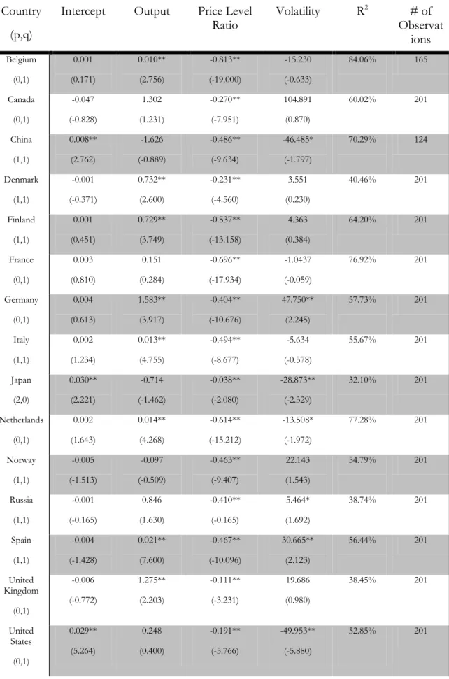
Table 5.1 and Table 5.3 summarise the results of the ordinary least square (OLS) regres-sions for Swedish bilateral exports and Swedish bilateral imports, respectively. The first column of the tables shows the applied autoregressive moving average (ARMA) structure. The autoregressive (AR) term refers to the number of lags of the dependent variable (p), and the moving average (MA) term refers to the number of lags of the error term (q) in-cluded in the regression. Moreover, the estimated parameter coefficient and the t-statistics (in parentheses) for each variable are included in the table. The last two columns display the R2 value and the number of observations for each regression.
Table 5.1: Regression Results of Swedish Exports
Country (p,q)
Intercept Output Price Level
Ratio Volatility R 2 # of Observat ions Belgium (0,1) 0.001 (0.171) 0.010** (2.756) -0.813** (-19.000) -15.230 (-0.633) 84.06% 165 Canada (0,1) -0.047 (-0.828) 1.302 (1.231) -0.270** (-7.951) 104.891 (0.870) 60.02% 201 China (1,1) 0.008** (2.762) -1.626 (-0.889) -0.486** (-9.634) -46.485* (-1.797) 70.29% 124 Denmark (1,1) -0.001 (-0.371) 0.732** (2.600) -0.231** (-4.560) 3.551 (0.230) 40.46% 201 Finland (1,1) 0.001 (0.451) 0.729** (3.749) -0.537** (-13.158) 4.363 (0.384) 64.20% 201 France (0,1) 0.003 (0.810) 0.151 (0.284) -0.696** (-17.934) -1.0437 (-0.059) 76.92% 201 Germany (0,1) 0.004 (0.613) 1.583** (3.917) -0.404** (-10.676) 47.750** (2.245) 57.73% 201 Italy (1,1) 0.002 (1.234) 0.013** (4.755) -0.494** (-8.677) -5.634 (-0.578) 55.67% 201 Japan (2,0) 0.030** (2.221) -0.714 (-1.462) -0.038** (-2.080) -28.873** (-2.329) 32.10% 201 Netherlands (0,1) 0.002 (1.643) 0.014** (4.268) -0.614** (-15.212) -13.508* (-1.972) 77.28% 201 Norway (1,1) -0.005 (-1.513) -0.097 (-0.509) -0.463** (-9.407) 22.143 (1.543) 54.79% 201 Russia (1,1) -0.001 (-0.165) 0.846 (1.630) -0.410** (-0.165) 5.464* (1.692) 38.74% 201 Spain (1,1) -0.004 (-1.428) 0.021** (7.600) -0.467** (-10.096) 30.665** (2.123) 56.44% 201 United Kingdom (0,1) -0.006 (-0.772) 1.275** (2.203) -0.111** (-3.231) 19.686 (0.980) 38.45% 201 United States (0,1) 0.029** (5.264) 0.248 (0.400) -0.191** (-5.766) -49.953** (-5.880) 52.85% 201
In the case of Swedish exports (Table 5.1), we find that the control variables output and price level ratio are significant in most cases and generally display their expected signs. Output is significant in nine cases, and price level ratio is significant in all cases. Price level ratio always displays the expected negative sign. Output, however, is positive in all but three cases, where none of the negative signs shows significance.
The explanatory variables explain from 32% up to 84% of the variability in the export volumes.
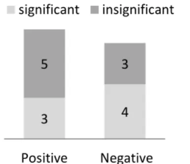
Exchange rate volatility has a significant impact on export volumes in seven out of the fifteen cases (China, Germany, Japan, the Netherlands, Russia, Spain & USA). We find a positive relationship in three cases (Germany, Russia & Spain) and a negative in four cases (China, Japan, the Netherlands & USA). These results are summarised in Figure 5.1.
These mixed results are in line with previous research and demand further analysis. We focus on Swedish exports first, then on imports and give possible explanations for the large number of insignificant results. We seek to find explanations in the argumentations of the theoretical framework for our results.
According to the model by De Grauwe (1988) the sign of the relationship between exchange rate volatility and trade flows depends on the level of risk-aversion. While moderate levels of risk-aversion lead to a negative relationship, high levels of risk-aversion cause the trade flows to increase with an increase in the volatility of the exchange rate. There is no widely used measure of risk-aversion for countries. However, Holzhausen and Scorbureanu (2011) developed the Composition Index of Propensity to Risk (CIPR) as a measure for the attitude towards risk in a country. Unfortunately, the CIPR, which can be found in Table 5.2, is not available for Canada, China, and Russia. The higher the displayed CIPR, the higher is the degree of risk-aversion. A negative CIPR indicates risk-seeking behaviour, while a CIPR close to zero indicates risk-neutral behaviour. As mentioned by Qian and Varangis (1994), some of Swedish exports are priced in the domestic currency. Therefore, the importers of these goods bear the exchange rate risk. Thus, we look at the risk-aversion of both trading partners and not just on the exporters’. According to the CIPR, German firms are very risk-averse. The model by De Grauwe (1988) would therefore predict a positive effect of exchange rate volatility on Swedish exports to Germany. This is in line with our regression estimates for Germany. The results for Japan and the Netherlands also seem to support this
Table 5.2: Composition Index of Propensity to Risk
Country CIPR Relative level of risk-aversion
USA -0,037 risk-neutral Italy 0,068 risk-neutral Spain 0,072 risk-neutral Japan 0,107 moderate risk-averse Sweden 0,109 moderate risk-averse UK 0,121 moderate risk-averse France 0,152 moderate risk-averse Netherlands 0,160 moderate risk-averse Belgium 0,163 moderate risk-averse Norway 0,174 very risk-averse Denmark 0,176 very risk-averse Finland 0,191 very risk-averse Germany 0,241 very risk-averse
Source: Holzhausen & Scorbureanu (2011)
Figure 5.1: Exports: Estimated
Signs for Volatility.
3 4
5 3
Positive Negative
model. Both countries have moderate levels of risk-aversion, and our empirical test finds a negative effect of exchange rate volatility on the Swedish export volume to Japan and the Netherlands. According to the CIPR value, Spain is risk-neutral but we find a positive relationship between exchange rate volatility and growth in export volume. De Grauwe (1988), however, assumes that risk-neutrality, does not exist.
For certain industries, the model developed by Broll and Eckwert (1999) predicts a positive relationship between exchange rate volatility and exports. As an example, they mention the agricultural sector. Our empirical tests find significant and positive relationships for Russia and Spain. They import, compared to other countries, a relatively large share of agricultural products from Sweden. This seems to indicate that the model by Broll and Eckwert (1999) can explain the sign of this relationship. However, the share of agricultural products of the total Swedish exports to Germany, for which we also find a significant, positive relationship, is relatively small. The shares of Swedish export volumes of goods by industry for the significant regressions can be found in Appendix: Analysis in Table A 5. A more effective way to test the Broll-Eckwert model (1999) would be to investigate this relationship at a sectoral rather than country level. However, we consider the assumption of the Broll and Eckwert (1999) model that exporters can sell all their products in the domestic market to be too limiting in Sweden’s case. Sweden is a small economy, and therefore, we cannot assume that all exporters would be able to sell all their goods in the domestic market at any given moment (SCB).
The results for our regressions of Swedish imports are summarised in Table 5.3. We find that our control variables output and price level ratio are significant in most cases, and if they are significant, they have the expected signs. The values for R2 vary from
approximately 37% in the case of Russia to 91% in the case of Japan. For some countries where only the growth of price level ratios is significant (Canada, Japan & USA), the high R2 values seem suspicious. However, we conduct statistical tests and find no problems. The
R2 values can be explained by the use of an ARMA structure, which usually leads to high R2
values, as well as the relatively strong correlation of the growth of price level ratios to the growth of imports.
The estimated parameter coefficients for the volatility variable take on negative values in nine cases, while they are positive in six cases. However, the coefficients are only significant in two cases. These results are summarised in Figure 5.2. Swedish imports from Germany are positively affected by the volatility of the exchange rate. On the other hand, we find that the volatility of the exchange rate between the euro and the Swedish krona seems to have a negative impact on the volume of Swedish imports from Italy.
When comparing the model by De Grauwe (1988) to our empirical findings, we find that the model is in line with
the estimated sign for Swedish imports from Germany. Germany’s high risk-aversion according to the CIPR (Table 5.2) and positive impact of exchange rate volatility on the exports to Sweden is in line with the model.
In the Italian case, we do not find any empirical evidence to support the model. Italy’s CIPR indicates risk-neutrality, and De Grauwe’s model does not make predictions for the relationship between exchange rate volatility and trade for risk-neutral trading partners.
Figure 5.2: Imports: Estimated
Signs for Volatility.
1 1
5
8
Positive Negative
Table 5.3: Regression Results of Swedish Imports
Country (p,q)
Intercept Swedish
Output Price Level Ratio Volatility R
2 # of Observat ions Belgium (6,0) 0.003 (0.725) 1.379** (4.236) -0.110** (-3.692) -6.601 (-0.335) 55.28% 165 Canada (0,1) -0.013 (-0.390) 1.222 (1.610) -0.738** (-21.558) -24.965 (-0.355) 83.17% 201 China (0,1) 0.006 (1.906) 0.848 (0.284) -0.522** (-10.874) -83.395 (-1.167) 74.95% 124 Denmark (1,1) -0.004 (-0.980) 0.944** (2.814) -0.948** (-18.019) 17.734 (1.059) 76.71% 201 Finland (1,1) 0.005** (2.693) 0.615** (2.542) -0.342** (-6.219) -14.856 (-1.486) 41.81% 201 France (0,1) 0.003 (1.477) 0.611** (2.433) -0.296** (-7.942) -13.830 (-1.239) 56.94% 201 Germany (1,1) -0.008** (-2.087) 1.346** (4.184) -0.626** (-15.400) 36.771** (2.176) 67.53% 201 Italy (0,2) 0.005** (2.000) 1.161** (4.777) -0.340** (-7.470) -19.915* (-1.832) 53.64% 201 Japan (1,1) 0.215 (1.325) -0.154 (-0.199) -0.943** (-31.821) -18.462 (-1.039) 91.44% 201 Netherlands (0,1) -0.002 (-0.600) 0.481* (1.778) -0.326** (-9.130) -15.312 (-0.293) 50.25% 201 Norway (0,1) 0.002 (0.168) 0.829** (2.300) -0.700** (-10.304) -9.686 (-0.181) 64.53% 201 Russia (1,1) 0.011 (0.753) 0.317 (0.150) -0.264** (-3.564) -1.026 (-0.081) 37.17% 201 Spain (1,1) -0.002 (-0.791) 1.396** (3.780) -0.468** (-10.506) 21.473 (1.378) 58.33% 201 United Kingdom (0,1) -0.005 (-0.487) 0.901** (2.896) -1.016** (-25.673) 11.108 (0.445) 86.43% 201 United States (1,1) 0.003 (0.293) 0.820 (1.445) -0.774** (-23.633) -6.880 (-0.418) 88.18% 201
We do, however, find that this relationship is both negative and significant.
There is no evidence to support Broll and Eckwert’s (1999) prediction concerning the relationship between exchange rate volatility and Swedish imports. Italy, for which we find a negative relationship, exports a relatively large amount of agricultural products (see Table A 6). Germany, on the other hand, exports a relatively small amount of agricultural products, but displays a positive relationship between volatility and export volume in our empirical test.
Obviously, not all countries display the negative effect of exchange rate volatility on Swedish trade flows that the Hooper-Kohlhagen (1978) model would expect. However, in two cases we estimate a negative relationship when both trading partners are risk-averse according to the CIPR. Sweden is a averse country, thus we never have a pair of risk-neutral countries.
This raises the question why our regressions estimate eight insignificant results for Swedish exports and thirteen insignificant results for Swedish imports. One explanation for the fact that we find more significant results for Swedish exports than Swedish imports might be that Sweden is a small open economy (Bergin, 2006).
One of Hooper and Kohlhagen’s (1978) assumptions may give an indication as to why we obtain these results. They assume that no vehicle currencies are used. It may be possible that the use of a third currency to conduct trade in caused some of our insignificant results. We have only measured bilateral exchange rate volatility but for some exporters and importers the volatility in a vehicle currency has actually far greater effects. Friberg (1999) finds that only 33.1% of imports and 43.8% of exports were priced in Swedish krona in 1995. Wilander (2004) finds that in 2002 25.5% of Swedish exports are invoiced in a vehicle currency, while 39.4% are invoiced in Swedish krona and the rest in the local currencies of the trading partners. The use of vehicle currencies varies among industries: The motor vehicle industry used them only in 2.6% of invoices while the paper and pulp industry used them in 48.0% of invoices in 2002. Thus, trade flows that are characterised by industries that rely heavily on vehicle currencies may be more influenced by volatility in the vehicle currency than in the bilateral exchange rate. The difference in use of invoicing currencies between exports and imports could also explain the different results we obtain for exports and imports.
Therefore, we rerun our regressions with the inclusion of the volatility measures for the bilateral exchange rates with the two major vehicle currencies (U.S. dollar and euro) as additional explanatory variables (Kamps, 2006). For these regressions, we use the following equation: ∑ ∑ (5.4)
We find that vehicle currencies have a significant effect in seven cases. Table A 7 and Table A 8 in Appendix: Analysis summarise the regression results for these cases. The tables are constructed in the same manner as Table 5.1 and Table 5.3. We summarise the estimated signs for the significant vehicle currency coefficient parameters for exports and imports in Figure 5.3.
Figure 5.3: Estimated Signs for
Significant Vehicle Cur-rencies. 2 1 2 2 Exports Imports
Positive Negative We observe a significant relationship of U.S. dollar
volatility with Swedish exports in three cases (Italy, Spain & UK) and with Swedish imports in two cases (Norway & Spain). The volatility of euro has a significant effect on Swedish exports to the U.S. and on Swedish imports from Canada. We find an equal amount of positive and negative relationships.
This indicates that because of the use of vehicle currencies one should not only consider bilateral exchange rate volatility. The volatility in the exchange rate with the vehicle currency has therefore some effect on international trade flows.
There are several other possible explanations why we obtain insignificant results. Hedging could be an issue since Swedish firms hedge about 50% of their expected sales against exchange rate risk (Friberg, 2008). Also, volatility might not be as important for multinational corporations. Large corporations account for 52% of Swedish exports (Friberg & Wilander, 2008). It is also possible that import demand is inelastic in the short-run.
Returning to our original question, whether one of the three presented models explains trade flows well, we have to answer: no. There is some evidence that De Grauwe (1988), Hooper and Kohlhagen (1978) as well as Broll and Eckwert (1999) correctly identified some determinants of the effects of exchange rate volatility on trade flows. All of them might be correct in explaining some aspects of this relationship. It seems certain that none of the models captures all the effects of exchange rate volatility and that different factors dominate different trade flows. It appears that the relationship between exchange rate volatility and trade flows is a complex one. A more complex one than the presented theoretical models consider. It is complicated to predict effects of exchange rate volatility due to the realities of hedging, vehicle currencies, and the various incentives available for large corporations in an international environment. This makes it difficult for policy makers to draw conclusions. However, due to the availability of financial derivatives, the effect of exchange rate volatility on trade flows does not have to be one of the main concerns for policy makers in determining the optimal exchange rate regime. Besides, the mixed results of contemporary research would make policy recommendations difficult.
Our significant as well as insignificant results give reasons for future research. Especially the numerous insignificant results for Swedish imports call for further investigation. That is, however, outside of the scope of this thesis. Thus, we finish this thesis in the next section with suggestions for future research as well as some concluding remarks.