Marginal Railway Infrastructure Costs in a Dynamic
Context
Mats Andersson
VTI, Box 760, 781 27 Borlänge, Sweden
E-mail: mats.andersson@vti.se
Abstract
In this paper, dynamic aspects of railway infrastructure operation and maintenance costs in Sweden are explored. Econometric cost functions are estimated to check the robustness of previous marginal cost estimates by introducing lags and leads of both dependent and independent variables. We find support for a forward-looking behaviour within the Swedish National Rail Administration (Banverket) as both infrastructure operation and maintenance costs are reduced prior to a major renewal. There are also indications of both lagged traffic and costs affecting the cost structure, but these results are more uncertain due to limitations in data.
Keywords: Railway, Infrastructure Operation, Maintenance, Marginal Costs, Dynamic
Panel Data.
1. Introduction
Marginal cost estimation of railway infrastructure wear and tear is an important task in the light of the European railway policy. Andersson (2006, 2007a, 2007b) estimates the marginal cost of wear and tear in Sweden using pooled ordinary least squares (POLS), fixed effects (FE) and survival analysis (SA). Although these models all include a variety of traffic and infrastructure variables, they exclude dynamic aspects on the cost structure i.e. they ignore the possibility of the cost level in time t to be affected by costs or other aspects in other time periods, t ± m.
The purpose of this paper is to extend the work in Andersson (2006, 2007a) by introducing lags and leads of dependent and independent variables as an explanation for railway infrastructure costs in Sweden. We make use of both static and dynamic panel data models
when exploring potential dynamic effects. This provides an indication of how robust previous elasticity and marginal cost estimates are.
The outline of the paper is as follows. Section 2 makes a brief review of previous work in this field followed by a description of our data in section 3. Hypothesis of dynamics are explored in section 4. The econometric models and associated results are presented in section 5, and we discuss the results and draw conclusions in section 6.
2. Literature review
This paper builds on recent work on the cost structure of vertically separated railway organisations. There has been increasing activity in the field of marginal railway cost estimation in Europe during the last decade (Link and Nilsson, 2005). This has grown out of a sequel of projects funded by the European Commission in line with the European railway policy (European Parliament, 2001). The work so far has been devoted to setting the framework for transport system pricing (Nash and Sansom, 2001), linking cost accounts in member states to match the needs of marginal cost estimation (Nash, 2003), finding best practices in member states (Thomas et al., 2003) and disseminating findings (Nash and Matthews, 2005). Still, there is only a limited number of empirical studies undertaken related to marginal railway infrastructure costs using micro-level data (Lindberg, 2006).
The paper that initiated both recent and current research is Johansson and Nilsson (2004)1. They estimate cost functions on data from Sweden ranging from 1994 to 1996, and from Finland between 1997 and 1999. Johansson and Nilsson (2004) apply the method of pooled ordinary least squares (POLS) in their analysis. Pooling the annual data and using a restricted version of the Translog specification by Christensen et al. (1973), they derive cost elasticities
1 The work by Johansson and Nilsson was done in the late 1990’s and the working paper that circulated then
with respect to output and associated marginal costs. The approach by Johansson and Nilsson (2004) to use infrastructure costs as dependent variable, and traffic variables as well as infrastructure standard as independent variables is used in most research recently (Munduch et al., 2002; Daljord, 2003; Tervonen and Idström, 2004; Andersson, 2006; Marti and Neuenschwander, 2006; Smith and Wheat, 2006)2. Traffic volumes in terms of gross tonnes and trains are considered as outputs of the track, and costs are assumed to be minimised for a given level of output.
Munduch et al. (2002) use 220 annual observations from the Austrian Railways between 1998 and 2000. The data consists of track maintenance costs, traffic volumes in gross tonnes, and a rich set of infrastructure variables. Pooled estimates are compared to annual estimates and tests favour the former. They also test for and reject the use of tonne kilometres as output, and suggest tonnes and track kilometres as separate variables.
Daljord (2003) estimates Cobb-Douglas and Translog functions on Norwegian maintenance cost data from 1999 to 2001, but he is heavily restricted in his analysis by data availability. The Translog specification is rejected on the grounds of theoretically un-sound predictions in favour of the Cobb-Douglas. He concludes that there is a need for a dedicated data collection strategy in Norway to come to terms with the evident problems in the data used.
Tervonen and Idström (2004) analyse the cost structure of the Finnish railway network with data from 2000 to 2002, using a Cobb-Douglas function. They differ in their approach by a priori identifying fixed and variable cost groups, and only analysing variable costs. The analysis is based on maintenance costs as well as an aggregate of maintenance and renewal. Their main conclusion is that marginal costs have decreased compared to analyses undertaken
on data from 1997 to 1999, but the reduction might come from inconsistencies in the cost accounts.
Andersson (2006) updates the estimates by Johansson and Nilsson (2004) with data from 1999 to 2002 and finds that a separation of maintenance and infrastructure operation costs is warranted as the latter is driven by trains rather than gross tonnes3. The new data set also includes renewal costs, and models are estimated for maintenance only as well as an aggregate of maintenance and renewal.
Marti and Neuenschwander (2006) estimate a POLS model for maintenance cost data on the Swiss national network during 2003-2005. A rich set of infrastructure variables and traffic is used to explain cost variation.
While the studies above make use of micro-level data (track sections), the study by Smith and Wheat (2006) use data from 53 maintenance delivery units for the Great British Network in 2005/06 and apply OLS. They find somewhat higher elasticities than the other studies.
Considering the variation between the individual studies, the results have been reasonably similar in terms of cost elasticities with respect to (wrt) output, when controlling for the cost base included (Wheat, 2007). There seems to be evidence for the maintenance cost elasticity wrt output of gross tonnes to be in the range of 0.2 - 0.3, i.e. a 10 percent change in output gives rise to a 2-3 percent change in maintenance costs.
Lately, there has been some alternative econometric approaches to the one suggested by Johansson and Nilsson (2004). Gaudry and Quinet (2003) use a very large data set for French railways in 1999, and explore a variety of unrestricted generalised Box-Cox models to allocate maintenance costs to different traffic classes. They reject the Translog specification as being too restrictive on their data set. Andersson (2007a) estimates infrastructure operation
and maintenance cost models with fixed effects and rejects the pooled OLS approach. He finds significant heterogeneity in the data and estimates marginal maintenance costs twice as high as previous estimates in Andersson (2006) using POLS.
Based on discussions with staff at the Swedish National Rail Administration (Banverket), we have reason to believe that the cost structure have a dynamic structure, which could affect the previously estimated models. We explore some dynamic hypotheses in section 4, but first take a brief look at the data at hand.
3. Data
A panel (a combination of cross-sectional and time-series data) of track section data with cost, infrastructure and traffic information on the Swedish railway network over 1999-2002 will be analysed. This data has previously been used in Andersson (2006, 2007a) for cost function estimations, but is for this study extended to include renewal costs in 2003 and 2004. The analysis will be on the main part of the data set, 1999-2002, which are the only years for which we can observe traffic and infrastructure covariates. Extending the data with renewal costs for following years, implicitly assumes that the main characteristics of the track sections have been unchanged up to 2004. This assumption may not be too restrictive since the development of a railway network is a slow process. Andersson (2007a) estimated infrastructure characteristics as a fixed effect for 1999-2002; a decision based on the idea that within-track section variation is very small or non-existing for observed infrastructure variables.
3 Infrastructure operation was chosen in Andersson (2006) as the terminology used for short-term maintenance
The traffic data comprises gross tonne volumes and number of trains per track section, which are observed between 1999 and 2002.
4. Hypotheses of dynamics
There are some a priori hypotheses for believing that there might be underlying dynamic effects in our data, and a variety of model specifications are used in order to test these hypotheses. Models with lags and leads of both dependent and independent variables are explored; hence different models are used for different questions posed.
The first hypothesis is that infrastructure operation and maintenance costs in time t depend not only on covariates in time t, but also on whether a major renewal is being planned in t+1
or . This forward-looking behaviour could be part of a cost-minimising strategy, which includes reducing infrastructure and maintenance costs as the time of a track renewal is approached. Reducing maintenance costs could eventually lead to increased track degradation and derailment risks, but common knowledge within track managers’ circles is that this strategy is safe to run for a few years. Thus, the hypothesis is that future renewal costs will
lead current infrastructure operation and maintenance costs. Dummy variables for major
renewals, , are generated based on a comparison of annual maintenance costs in t, , and annual renewals in ( ), , and
2 + t R m it D , CitM 1 +
t m=1 CitR+1 t+2 (m=2), , for each observation. If renewal costs are equal to or larger than maintenance costs, this is identified as a major renewal (1). R it C +2 ⎪⎩ ⎪ ⎨ ⎧ = ≤ = > = + + 2 , 1 if 1 2 , 1 if 0 , m C C m C C D R m it M it R m it M it R m it (1)
A negative relationship between maintenance costs in t and major renewals in t+1 and t+2 is expected, but there are uncertainties a priori about what effect this forward-looking behaviour will have on infrastructure operation costs, if any. Apart from winter maintenance, infrastructure operation involves short-term maintenance, which one can suspect either to increase or decrease as a reaction to reduced maintenance. A carefully planned reduction in maintenance will open up for a parallel reduction in infrastructure operation costs, but if the maintenance reduction is taken too far we might also observe increased infrastructure operation costs as a backlash.
This analysis poses no specific problems related to the econometric model specification. The dummy variables for renewals are exogenous variables and this model can be estimated using a fixed effects estimator as in Andersson (2007a).
T t N i yit =xit′β+z′iα+εit, =1,2,..., =1,2,..., (2)
y is our dependent variable, x is a vector of explanatory variables, z is a vector that captures
observed or unobserved heterogeneity and ε is the error term. If in (2) contains an unobserved effect that is correlated with , we can use an individual specific constant,
i z it
x αi,
as in expression (3) to get unbiased and consistent estimates of all model parameters. See Wooldridge (2002) or Greene (2003) for an exhaustive presentation of fixed effects estimation. T t N i yit =αi +xit′β+εit, =1,2,..., =1,2,..., (3)
The second hypothesis is that maintenance costs in t might be affected by traffic not only in t, but also in t - 1. Hence, we assume that there is some reaction time for actions in response to observed traffic levels. The short time panel available is a restriction and the analysis is therefore limited to a one-year lag structure. A variety of specifications for maintenance costs will be investigated. This hypothesis will also be analysed using the fixed effect model in (3), but is not applied to infrastructure operation costs, as it is hard to justify such a dynamic relationship for short-term and winter maintenance.
The third hypothesis is linked to the nature of maintenance itself. Some maintenance activities are not needed on an annual basis, which means that there will be fluctuations in maintenance costs between years, even if traffic volumes are constant. If too little is spent on maintenance one year it will come out as a need to spend more the coming year. This cyclic behaviour will continue in order to keep the railway track in a steady-state condition over time. If this hypothesis holds, costs in year t depend on costs in year t−1, and exploring a lag
structure of the dependent variable is warranted. For this type of cyclic fluctuations, we expect a negative coefficient for the lagged variable, and for the process to be stationary the estimated coefficient has to be between -1 and 0 (Vandaele, 1983). The size of the coefficient signals the importance of historical maintenance. The further away from 0, the more important is the history. A positive estimate indicates a trend in costs over time, while a negative estimate shows that the cost is oscillating around some mean value over time. Once again, this hypothesis is not applied to infrastructure operation costs.
The third hypothesis introduces special problems with autocorrelation between the error term and the lagged dependent variable through the group specific effect, but Arellano and Bond (1991) suggested a generalised method of moments (GMM) estimator for this type of problem, which involves taking first differences of the model to sweep away heterogeneity in the data.
Consider a model where a dynamic relationship in y is captured through a lagged dependent variable as a regressor (4), T t N i y yit =δ it−1+x′itβ+εit, =1,2,..., =1,2,..., (4)
where δ and β are parameters to be estimated, xit is a vector of explanatory variables for
observation i in time t, is a vector . Assume that the error term εit follows a one-way error
component model εit =µi +νit where µi is IID (0, σµ2) andνit is IID (0, ) independent of
each other and among themselves.
2
ν
σ
This model will include two effects that persist over time, autocorrelation from using a lagged dependent variable and heterogeneity from the individual effect µi. Autocorrelation
comes from yit being a function of µi and subsequently yit-1 also being a function of µi.
Therefore, the regressor yit-1 in (4) is correlated with the error term εit. This will make an OLS
regression biased and inconsistent. Furthermore, Baltagi (2005) shows that both standard FE and RE estimation of expression (4) will be biased, but a solution proposed to these problems is first-differencing, which will wipe out the individual effect and using lagged instruments to handle the autocorrelation. An instrument is a variable that does not itself belong to the regression, that is correlated with yit-1, and that is uncorrelated with εit.
Arellano and Bond’s (1991) dynamic panel data estimator does exactly the above, but also use the orthogonality between lagged values of yit and νit to create additional instruments.
A simple autoregressive version of (4) with the same error structure, but without regressors, is given in (5).
T t N i y yit =δ it−1+εit, =1,2,..., =1,2,..., (5)
To consistently estimate δ, take first differences of (5) to eliminate the individual effect µi,
which will make the second term on the right-hand side equal to zero.
) ( ) ( ) ( ) ( 1 0 2 1 1 − − − − = − + − + − − it it it i i it it it y y y y δ 6µ474µ8 ν ν (6)
In order to find valid instruments to the lagged differenced regressor (that are uncorrelated with the differenced error term), T ≥ 3 is needed. T = 3 gives the following model (7),
) ( ) ( ) (yi3−yi2 =δ yi2 −yi1 + νi3−νi2 . (7) 1 i
y is highly correlated with (yi2−yi1) and a valid instrument, but at the same time
uncorrelated with (νi3−νi2). If T is extended, the list of instruments is extended. With T = 4, both yi1 and yi2 are valid instruments to the regressor (yi3−yi2) and one can go on like
this by adding more instruments as T increases.
If we add other regressors ( ) that are correlated with the individual effect to the Arellano and Bond model, then these can also be used as instruments if they are strictly exogenous with it x . , ... 2, 1, , 0 ) ( t s T
E xitεis = ∀ = This approach can also be adjusted if some or all
instruments are considered predetermined otherwiseE(xit εis)≠0for t<s ,andzero (see chapter 8 in Baltagi, 2005 for further details).
5. Model specifications and estimation results
The hypotheses presented in section 4 are incorporated into econometric models that can be estimated using either static or dynamic panel data estimators. Models and results for infrastructure operation are presented in section 5.1, and for maintenance in section 5.2. All model estimations are done using Stata 9.2 (StataCorp, 2005) and costs are expressed in 2002 real prices.
5.1 Infrastructure operation costs
In this sub-section, a model for infrastructure operation costs in the presence of renewal leads is explored. This model is an extension of the suggested model in Andersson (2007a) and fixed effects at track section level are assumed.
Model 1 is for infrastructure operation costs using a third-degree polynomial for the natural
logarithm of trains (TT) and dummy variables for future renewals ( ). A model with dummy variables for renewals in both t+1 and t+2 has been tested, but the coefficient for the renewal in t+2 is insignificant. Based on Akaike’s Information Criterion (AIC), the specification with two dummy variables is rejected in favour of a reduced model given in expression (8). Fixed effects (FE) at track section level are captured in
R m it D , i α , and εit is the homoscedastic error term with zero mean. The estimates of the reduced model are given in table 1. it R it it it it i O it TT TT TT D C =α +β1ln +β2(ln )2 +β3(ln )3+φ1 ,1+ε ln (8)
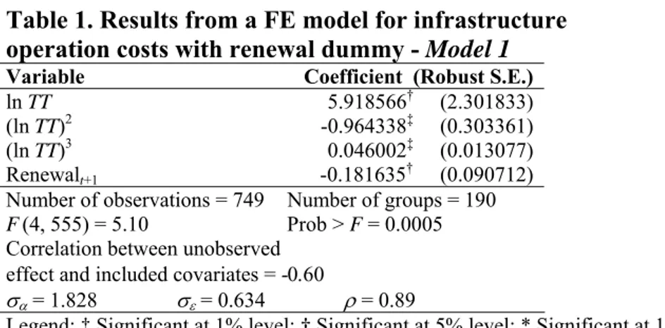
Table 1. Results from a FE model for infrastructure operation costs with renewal dummy - Model 1
Variable Coefficient (Robust S.E.)
ln TT 5.918566† (2.301833)
(ln TT)2 -0.964338‡ (0.303361)
(ln TT)3 0.046002‡ (0.013077)
Renewalt+1 -0.181635† (0.090712)
Number of observations = 749 Number of groups = 190
F(4, 555) = 5.10 Prob > F = 0.0005
Correlation between unobserved effect and included covariates = -0.60
σα = 1.828 σε = 0.634 ρ = 0.89
Legend: ‡ Significant at 1% level; † Significant at 5% level; * Significant at 10% level.
The overall model is significant at the 1 percent level based on the F test. There is a strong correlation between the unobserved effect and our included covariates (-0.6). The importance of the unobserved fixed effect can be measured as (Wooldridge, 2002). ρ is estimated to 0.89, i.e. almost 90 per cent of the variation is contributed to the variation in our unobserved effect. We also reject the model in Andersson (2007a) based on the AIC.
) /( 2 2 2 ε ε α σ σ σ ρ = +
The calculation of individual cost elasticities is based on expression (9), which is the derivative of the estimated cost function with respect to the output variable4. The standard error of the elasticity is computed using the Delta method (Greene, 2003, Appendix D.2.7).
) ) (ln ˆ 3 ( ) ln ˆ 2 ( ˆ ˆ 2 3 2 1 it it O it =β + ⋅β ⋅ TT + ⋅β ⋅ TT γ (9)
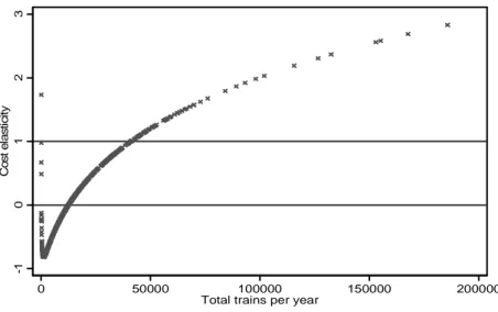
The point estimate of the output elasticity is negative at -0.017 (standard error 0.19), but if we look at individual estimates, they range from negative to positive (figure 1).
4 This follows from the model specification using the logarithm of costs as dependent variable and logarithm of
-1 0 1 2 3 C o st el as ti ci ty 0 50000 100000 150000 200000 Total trains per year
Figure 1. Infrastructure operation cost elasticity wrt output – Model 1
In fact, low volume tracks have negative elasticities, but at 12,000 trains per year (an average of close to 33 trains per day) the sign shifts from negative to positive. This means that trains contribute positively to winter maintenance up to a certain level, but this positive effect is exhausted as volumes exceed this threshold. This finding is in line with Andersson (2007a) and a commonly held view in the Swedish railway industry, that trains help to sweep the snow of the track. Furthermore, the elasticity exceeds 1 as output volumes approaches 40,000 trains per year, i.e. we turn from economies to diseconomies of density (Caves et al., 1985). At high volumes costs increase more than proportionally to the number of trains.
The coefficient for future renewals on infrastructure operation costs is -0.182 and significant at the 5 percent level. Since it is a dummy variable, the elasticity is calculated as . Hence, the effect from a renewal in t+1 is an infrastructure operation cost reduction by 17 percent in t (standard error 0.027). There is no evidence of increased infrastructure operation costs as a consequence of future renewals, but this has to be judged in the light of the estimates in our maintenance cost models in the next section.
1 ) ˆ exp(φ1 −
Average costs are calculated using expression (10), which is predicted costs divided by output kilometres at track section level. Marginal costs are calculated as the product between the output elasticity and the average cost (11).
it O it O it TKM C AC = ˆ (10) O it O it O it AC MC =γˆ ⋅ (11)
The mean of the average cost is SEK 7.26 (standard error 1.250) per train kilometre, while the mean of the marginal cost is negative at SEK -3.40 (standard error 0.940)5. This stems from high average costs and negative elasticities on track sections with low volumes that contribute heavily to the point estimate.
The calculated marginal costs from (11) are observation specific. If we adjust the marginal cost and estimate a mean value taking individual traffic levels into account, we get a weighted marginal cost for the entire network based on the traffic share per track section as in (12).
∑
∑
⎥ ⎥ ⎦ ⎤ ⎢ ⎢ ⎣ ⎡ ⋅ = it it it it O it O W TKM TKM MC MC (12)The weighted point estimate is SEK 0.121 (standard error 0.080) per train kilometre, but insignificantly different from zero at the 10 percent level.
5The exchange rate from Swedish Kronor (SEK) to Euro (EUR) is SEK 9.32/EUR and from Swedish Kronor to US
5.2 Maintenance costs
In this sub-section, models for maintenance costs are explored. Firstly, the effect on maintenance costs from future renewals is analysed. Secondly, we introduce lagged traffic variables and thirdly, add a lagged dependent variable to the model.
Maintenance costs and future renewals - Model 2
In a similar fashion as for infrastructure operation costs, a logarithmic model for maintenance costs (CM) is specified in expression (13), using total gross tonnes (TGT) as output variable.
Rail age is also added to the model. The reason for this is that we cannot argue for rail age to
be included in the time-invariant, group specific fixed effect for each track section as it changes over time per definition6. The third-degree polynomial specified in Andersson (2007a) remains valid when adding both dummy variables for future renewals. Estimates are given in table 2. it R it R it it it it it i M it D D RailAge TGT TGT TGT C ε φ φ β β β β α + + + + + + + = 2 , 2 1 , 1 1 3 3 2 2 1 ln ) (ln ) (ln ln ln (13)
The estimated coefficients have expected signs and are significant at the 5 per cent level (except the squared term with a prob. value of exactly 0.05). Both coefficients for the dummy variables for future renewals are significant at the 1 percent level, with coefficients just below -0.13 or in elasticity terms -0.12. Maintenance costs are reduced by approximately 12 percent per year when a renewal is planned within any of the coming two years.
Table 2. Results from a FE model for infrastructure maintenance costs and renewal dummies - Model 2
Variable Coefficient (Robust S.E.)
ln TGT 7.184414† (3.636894) (ln TGT)2 -0.547177* (0.278821) (ln TGT)3 0.013869† (0.006992) ln Rail age 0.144854† (0.064431) Renewal t+1 -0.129461‡ (0.037926) Renewalt+2 -0.125880‡ (0.042143)
Number of observations = 749 Number of groups = 190
F(6, 553) = 5.36 Prob > F = 0.0000
Correlation between unobserved effect and included covariates = 0.16
σα = 0.931 σε = 0.346 ρ = 0.88
Legend: ‡ Significant at 1% level; † Significant at 5% level; * Significant at 10% level.
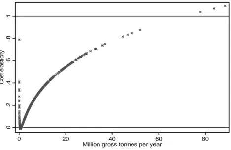
The mean cost elasticity with respect to output is estimated to 0.23 although only significantly positive at the 10 percent level (standard error 0.13). A plot of predicted elasticities is given in figure 2.
0 .2 .4 .6 .8 1 C o s t el as ti c it y 0 20 40 60 80
Million gross tonnes per year
Figure 2. Infrastructure maintenance cost elasticity wrt output – Model 2
Average costs, marginal costs and weighted marginal costs are calculated using expressions (10) – (12) with gross tonne kilometres used as output. The average cost per gross tonne
kilometre is SEK 0.09 and marginal cost SEK 0.014. The weighted marginal cost is estimated to SEK 0.0063 per gross tonne kilometre (standard error 0.00044).
Maintenance costs and lagged traffic - Model 3
The second model for maintenance analyses the effect of using lagged output as a covariate (14). We have also tried a model using both traffic volume in t and t-1, but the strong correlation between traffic over time forced traffic in t out of the model.
it R it R it it it it i M it D D RailAge TGT TGT C ε φ φ β β β α + + + + + + = − − 2 , 2 1 , 1 3 2 1 2 1 1ln (ln ) ln ln (14)
The third-degree polynomial for output used in Model 2 above is reduced to a second-degree, but all other variables remain in the model. One year of observations is lost when introducing lagged output to the model, and the sample size is reduced to 559 observations. The model results are given in table 3.
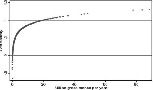
The F test indicates that we have a significant model and all coefficients have expected signs. The mean output elasticity is substantially higher than in Model 2 (0.629) and significantly above zero at the 1 percent level. The elasticities for future renewals are just a fraction lower than the estimates in Model 2. Model 3 estimates are -0.15 and -0.18 for t+1 and t+2 respectively, both significantly below zero at the 1 percent level. The output elasticity is increasing at a decreasing rate (figure 3), and exceeds 1 around 20 million gross tonnes per year. The economies of density are then exhausted.
Table 3. Results from a FE model for infrastructure maintenance costs, lagged traffic variables and renewal dummies - Model 3
Variable Coefficient (Robust S.E.)
ln TGTt-1 -2.460353 ‡ (0.974259) (ln TGTt-1)2 0.103196‡ (0.034956) ln Rail age 0.257608† (0.125642) Renewalt+1 -0.158292‡ (0.044992) Renewalt+2 -0.195988‡ (0.054259)
Number of observations = 559 Number of groups = 188
F(5, 366) = 9.40 Prob > F = 0.0000
Correlation between unobserved effect and included covariates = -0.38
σα = 0.981 σε = 0.360 ρ = 0.88
Legend: ‡ Significant at 1% level; † Significant at 5% level; * Significant at 10% level.
-. 5 0 .5 1 1. 5 C o s t el as ti c it y 0 20 40 60 80
Million gross tonnes per year
Figure 3. Infrastructure maintenance cost elasticity wrt output – Model 3
Following the increase in output elasticity, marginal cost estimates are much higher in this model, with a weighted estimate at SEK 0.016 (standard error 0.0009) per gross tonne kilometre. This is more than twice as high as the estimate in Model 2.
Maintenance costs and lagged costs - Model 4
The final model deals with the possibility of maintenance costs in t-1 affecting costs in t. The relatively short panel means that using a dynamic panel data specification for data from 1999
to 2002 will result in losing two full years of observations. The final sample consists of 371 observations.
There is a risk of an over-identified specification when using the Arellano and Bond estimator, i.e. the number of instruments exceeds the included regressors. Testing for over-identifying restrictions is a way of controlling the validity of the included instruments. There is though a possibility that a rejection of the instruments comes from violating the conditions of homoscedasticity, rather than weak instruments. A solution is then to use a two-step estimator (StataCorp, 2005) for model validation, but a one-step estimator for parameter inference. Furthermore, second-order autocorrelation in the residuals would lead to inconsistent estimates and needs to be tested for too.
The suggested model is given in (15) and builds on Model 3. The difference is the inclusion of lagged costs as an explanatory variable and a dummy for 2002 to pick up systematic differences between 2002 and 2001. Results from both one-step (Model 4a) and two-step (Model 4b) estimations are given in table 4.
it i it R it R it it it it M it M it D D D RailAge TGT TGT C C ν µ φ φ φ β β β β + + + + + + + + = − − − 2002 3 2 , 2 1 , 1 4 2 1 3 1 2 1 1 ln ) (ln ln ln ln (15)
We do not reject the null hypothesis of no first-order autocorrelation in the differenced residuals in either Model 4a or 4b. The short panel makes the test for second-order autocorrelation impossible to perform as the residuals in t and t-2 have no observations in common.
Using the Sargan test for over-identifying restrictions, we cannot reject the null hypothesis that the instruments are valid based on Model 4b. In Model 4a we reject the validity of the
alternatives. Still, inference on individual coefficients is based on Model 4a as suggested by StataCorp (2005).
Table 4. Results from 1-step and 2-step Arellano & Bond dynamic panel data estimators for infrastructure maintenance costs - Model 4a and 4b
Variable Arellano & Bond 1-step
Coeff. (S.E.) Arellano & Bond 2-step Coeff. (S.E.)
ln CMt-1 -0.558435‡ (0.163820) -0.615749‡ (0.203364) ln TGTt-1 -1.485938† (0.663649) -1.625028‡ (0.570388) (ln TGTt-1)2 0.059787† (0.026546) 0.063149‡ (0.023793) ln Rail age 0.087277 (0.105464) 0.084911 (0.090911) Year 2002 0.244428‡ (0.055466) 0.215424† (0.045803) Renewalt+1 -0.110589* (0.060079) -0.100959‡ (0.045731) Renewalt+2 -0.137055† (0.059185) -0.135058‡ (0.048814) Observations 371 371 Groups 186 186 Wald χ2 (7 df) 68.45 66.18 Sargan’s χ2 (2 df) 9.65; p > χ2 = 0.008 3.44; p > χ2 = 0.179 Autocov. Order 1 -0.89; p > z = 0.373 -0.52; p > z = 0.604 Autocov. Order 2 - -
Legend: ‡ Significant at 1% level; † Significant at 5% level; * Significant at 10% level.
The coefficient for our lagged cost variable is negative and significant from zero at the 1 percent level in the one-step model. We notice a strong negative relationship between the first-difference in costs between t-1 and t. A 10 percent increase in the difference of maintenance costs in t-1 generates a 5.5 percent cost reduction in t. This supports the hypothesis that costs are oscillating around a mean over time to keep the track in steady-state. Since the estimate of β1 <1, we have a stationary process (Vandaele, 1983).
The dynamic model gives us the possibility to calculate both short-run and long-run cost elasticities wrt output. The short-run elasticity is calculated as in the previous sections, but the formula for the long-run elasticity is slightly different. Based on our specification in (15), expression (16) gives us the long-run elasticity for infrastructure maintenance costs with respect to gross tonnes, with βˆ1 being the estimated coefficient for our lagged dependent
variable, and and our estimated output coefficients. The coefficient for our lagged dependent variable simply works as a scale factor between short-run and long-run effects.
2 ˆ β βˆ3
[
2 1 3 2 1 ) (ln ˆ 2 ˆ ) ˆ 1 ( 1 ˆ ⋅ + ⋅ ⋅ − − = it M LR β β TGT β γ]
(16)The second factor in the expression is equivalent to what we used in our analysis of lagged independent variables above. This is the short-run effect, or the short-run elasticity. The point estimate is calculated to 0.31 (standard error 0.192), but insignificantly different from zero, even at the 10 percent level. The long-run elasticity is lower due to the negative sign of the coefficient of our lagged dependent variable. A traditional definition of short-run and long-run cost elasticities is that in the short-long-run, the production technology is given, while in the long-run it is not. In our case, long-run is rather the effect from including the level of maintenance undertaken in a previous time period. A marginal change in traffic in t-1 will affect the level of maintenance in t-1, which in turn will affect the level of maintenance in t. This combined effect is captured in our long-run estimate.
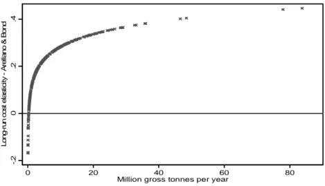
The point estimate of the long-run elasticity is 0.20 (standard error 0.128), but also insignificant from zero at the 10 percent level. Predicted elasticities are given in figure 4. To predict costs and calculate marginal costs from Model 5a, we need to look at the actual model that is estimated.
-. 2 0 .2 .4 Lo ng -r un c o s t e la s ti c it y A rel la no & B o nd 0 20 40 60 80
Million gross tonnes per year
Figure 4. Long-run infrastructure maintenance cost elasticity wrt output – Model 4a
) ˆ ˆ ( ) ( ˆ ) ( ˆ ) ( ˆ ) ln (ln ˆ ) ) (ln ) ((ln ˆ ) ln (ln ˆ ) ln (ln ˆ ) ln (ln 1 2002 1 2002 3 2 , 1 2 , 2 1 , 1 1 , 1 1 4 2 2 2 1 3 2 1 2 2 1 1 1 − − − − − − − − − − − − − + − + − + − + − + − + − + − = − it it it it R it R it R it R it it it it it it it M it M it M it M it D D D D D D RailAge RailAge TGT TGT TGT TGT C C C C ν ν φ φ φ β β β β (17)
Rearranging (17) to get on the left-hand side and replacing with our estimated coefficient, gives (18), which is used for prediction.
M it Cˆ ln βˆ1 ) ˆ ˆ ( ln 558 . 0 ln 442 . 0 ˆ ln = −1 + −2 +⋅⋅⋅+ it − it−1 M it M it M it C C C ν ν (18)
The section left out is simply the first-differences of our included variables multiplied with our estimated coefficients.
The estimated, weighted short-run marginal cost is SEK 0.0084 (standard error 0.00058) per gross tonne kilometre, which is 30 percent higher than in Model 2. The long-run estimate on the other hand is SEK 0.0054 (standard error 0.00037) per gross tonne-kilometre, which is 15 percent below the Model 2 estimate.
6. Discussion and conclusions
In this paper we have estimated econometric models for railway infrastructure costs in Sweden and tested the robustness of previous marginal cost estimates by introducing both lags and leads of dependent and independent variables in our cost functions. The general finding is that there seem to be dynamic characteristics that affect the cost structure of the Swedish railway network, but the available panel is too short to draw any strong conclusions. The first analysis concerns the effect on costs from planned future renewals and we find that both infrastructure operation and maintenance costs are reduced a couple of years prior to a large renewal. This confirms a forward-looking management strategy followed by Banverket, which is aiming at track maintenance cost minimisation. The effect that this has on our previous marginal cost estimates is not so large, but it is a dimension that needs to be taken into account in future modelling of railway infrastructure costs in Sweden and possibly other countries as well. A subsequent analysis to this would be to study if quality, measured as train delays and speed restrictions, can be maintained for train operators when costs are reduced for a limited time period.
The second analysis deals with the potential time delay between observed traffic volumes and maintenance activities. When introducing a one-year lag structure in our explanatory output variables, we experience the main problem of this dynamic analysis in the form of substantially different elasticities and marginal cost estimates compared to the previously used static models. We lose a full year of observations, which in this case is around 25 percent of the data. The model picks up a relationship between traffic in t and t-1, but it is difficult to draw any firm conclusions from this. The reason is the high correlation between traffic in t and t-1. The fact that traffic in t becomes insignificant in the model, when traffic in
from the effect from the reduced sample. A longer time-series for each track section (a wider panel) is needed for this analysis to be more reliable.
The final analysis focuses on lagged maintenance costs and once again we can see that the short panel is a problem. It is possible to estimate a dynamic panel data model for maintenance costs, but the available instruments are not so strong. Still, the short-run and long-run marginal cost estimates are not too far away from what is estimated in Andersson (2007a), or from the estimates in Model 2, which included the dummy variables for future renewals. We find support for a stationary cyclic spending pattern for maintenance, with a negative first-order autoregressive coefficient of -0.56. This is plausible as maintenance in t-1 can have a cost reducing effect on maintenance in t. It also shows that maintenance costs are kept around some level that keeps the track in steady-state. A wider panel could also solve some of the problems in this analysis and it is recommended for future research to try to extend the time window.
From the three analyses, the recommendation is to look closer at the results from Model 2; the inclusion of dummy variables for future renewals. This analysis indicates that the marginal cost for infrastructure operation costs is around SEK 0.12 per train kilometre as a weighted average. The equivalence for maintenance costs is SEK 0.0063 per gross tonne kilometre, which is twice as high as the current track charge for infrastructure wear and tear in Sweden; SEK 0.0029 per gross tonne kilometre (Banverket, 2006). There is no charge currently for infrastructure operation costs. Model 2 estimates are also in line with previous fixed effect estimates by Andersson (2007a). It seems like an application of marginal cost pricing would move the track charge in an upward direction. The other two analyses have promising features, and should be in focus for future research in this field.
If we look at the potential for cost recovery, a constant challenge for the transportation industry (Button, 2005), the marginal cost estimates leave a large part of costs spent on the
railway track uncovered. Cost recovery is defined as the ratio between marginal and average costs. However, this calculation has to be done at the track section level rather than comparing the two mean estimates since we have a non-linear relationship between output and cost.
Around SEK 1.3 billion is spent on railway maintenance every year in Sweden (Andersson, 2006). Charging SEK 0.0063 per gross tonne kilometre on a total of some 60 billion gross tonne kilometres per year would generate an income of SEK 378 million. Thus, the cost recovery rate would be around 30 percent if we assume that there would be no effect on the demand for train operations from the price increase. This is significantly higher than the current cost recovery rate in Sweden, which is as low as 5 percent. Scandinavian countries are also considered having the lowest wear and tear charges in Europe, which can explain the current low rate (Nash, 2005).
Our final conclusion is that dynamic aspects of rail infrastructure costs are important to explore further in the future, but such analyses require a data set that has a substantially longer time-frame in order to explore optimal lag structures of both dependent and independent variables. There is strong hope for improvements in that direction in Sweden as a new traffic data collection system has recently been implemented at Banverket. Combining this new information with both data that has been used in this study and data from the early 1990’s, we might be able to generate a data set that covers some 15 years and open up for improved dynamic analyses.
Acknowledgments
Financial support from Banverket is gratefully acknowledged. This paper has benefited from comments by Lars-Göran Mattsson, Jan-Eric Nilsson, Matias Eklöf and Jan-Erik Swärdh. The author is responsible for any remaining errors.
References
Andersson, M. (2006) Marginal Cost Pricing of Railway Infrastructure Operation, Maintenance and Renewal in Sweden: From Policy to Practice Through Existing Data.
Transportation Research Record: Journal of the Transportation Research Board, vol. 1943,
pp. 1-11.
Andersson, M. (2007a): Fixed Effects Estimation of Marginal Railway Infrastructure Costs in Sweden. Chapter 3 in Andersson, M. (2007) Empirical Essays on Railway Infrastructure
Costs in Sweden. Ph.D. Thesis. ISBN: 91-85539-18-X. Division of Transport and Location
Analysis, Department of Transport and Economics, Royal Institute of Technology, Stockholm, Sweden.
Andersson, M. (2007b): Marginal Railway Renewal Costs - A Survival Data Approach. Chapter 4 in Andersson, M. (2007) Empirical Essays on Railway Infrastructure Costs in
Sweden. Ph.D. Thesis. ISBN: 91-85539-18-X. Division of Transport and Location Analysis,
Department of Transport and Economics, Royal Institute of Technology, Stockholm, Sweden. Arellano, M. and Bond, S. (1991) Some Tests of Specification for Panel Data: Monte Carlo Evidence and an Application to Employment Equations. Review of Economic Studies, vol. 58, no. 2, pp. 277-297.
Baltagi, B.H. (2005) Econometric Analysis of Panel Data. 3rd ed., John Wiley & Sons, Chichester, UK.
Banverket (2006) Network Statement. 2006-12-10--2007-12-08(T07), Banverket, Market Division, Borlänge, Sweden.
Button, K. (2005) The Economics of Cost Recovery. Journal of Transport Economics and
Policy, vol. 39, no. 3, pp. 241-257.
Caves, D.W., Christensen, L.R., Tretheway, M.W. and Windle, R.J. (1985) Network Effects and the Measurement of Returns to Scale and Density for U.S. Railroads. Chapter 4 in Daughety, A.F. (ed.) Analytical Studies in Transport Economics. Cambridge University Press, Cambridge, UK, pp. 97-120.
Christensen, L., Jorgenson, D. and Lau, L. (1973) Transcendental Logarithmic Production Frontiers. Review of Economics and Statistics, vol. 55, no. 1, pp. 28-45.
Daljord, Ö.B. (2003) Marginalkostnader i Jernbanenettet. Report 2/2003, Ragnar Frisch Centre for Economic Research, Oslo, Norway.
European Parliament (2001) Directive 2001/14/EC of the European Parliament and of the Council of 26 February 2001 on the Allocation of Railway Infrastructure Capacity and the Levying of Charges for Use of Railway Infrastructure and Safety Certification. Official
Journal of the European Communities L 075, March 15, pp. 29-46.
Gaudry, M. and Quinet, E. (2003) Rail Track Wear-and-Tear Costs by Traffic Class in France. Paper presented at the First Conference on Railroad Industry Structure, Competition
and Investment, Nov. 2003, Toulouse, France.
Greene, W.H. (2003) Econometric Analysis. 5th ed. Prentice Hall, Upper Saddle River, NJ. Gujarati, D.N. (1995) Basic Econometrics. 3rd ed., McGraw-Hill, Singapore.
Johansson, P. and Nilsson, J.-E. (2004) An Economic Analysis of Track Maintenance Costs.
Transport Policy, vol. 11, no. 3, pp. 277-286.
Lindberg, G. (2006) Marginal Cost Case Studies for Road and Rail Transport. GRACE (Generalisation of Research on Accounts and Cost Estimation) Deliverable 3. Funded by 6th Framework RTD Programme. Institute for Transport Studies, University of Leeds, Leeds, UK.
Link, H. and Nilsson, J.-E. (2005) Infrastructure. Chapter 3 in Nash, C. and Matthews, B. (eds.) Measuring the Marginal Social Cost of Transport, Research in Transportation
Economics Vol. 14. Elsevier, Oxford, UK, pp. 49-83.
Marti, M. and Neuenschwander, R. (2006) Track Maintenance Costs in Switzerland. GRACE (Generalisation of Research on Accounts and Cost Estimation), Case study 1.2E. Annex to Deliverable D3: Marginal Cost Case Studies for Road and Rail Transport, Funded by 6th Framework RTD Programme. Ecoplan, Berne, Switzerland.
Munduch, G., Pfister, A., Sögner, L. and Stiassny, A. (2002) Estimating Marginal Costs for the Austrian Railway System. Working Paper 78, Vienna University of Economics and B.A., Department of Economics, Vienna, Austria.
Nash, C. and Matthews, B. (eds.) (2005) Measuring the Marginal Social Cost of Transport,
Research in Transportation Economics Vol. 14. Elsevier, Oxford, UK.
Nash, C. and Sansom, T. (2001) Pricing European Transport Systems: Recent Developments and Evidence from Case Studies. Journal of Transport Economics and Policy, vol. 35, no. 3, pp. 363-380.
Nash, C. (2005) Rail infrastructure charges in Europe. Journal of Transport Economics and
Nash, C. (2003) UNITE (UNIfication of accounts and marginal costs for Transport Efficiency), Final Report for Publication. Funded by 5th Framework RTD Programme, Institute for Transport Studies, University of Leeds, Leeds, UK.
Smith, A. and Wheat, P. (2006). Assessing the Marginal Infrastructure Wear and Tear Costs for Great Britain’s Railway Network. GRACE (Generalisation of Research on Accounts and Cost Estimation), Case study 1.2G. Annex to Deliverable D3: Marginal Cost Case Studies for Road and Rail Transport, Funded by 6th Framework RTD Programme. Institute for Transport Studies, University of Leeds, Leeds, UK.
StataCorp. (2005) Stata Statistical Software: Release 9. Longitudinal/Panel Data Reference Manual. College Station, Tx.
Tervonen, J. and Idström, T. (2004) Marginal Rail Infrastructure Costs in Finland 1997 –
2002. Finnish Rail Administration, Publication A 6/2004, Helsinki, Finland.
Thomas, J., Dionori, F. and Foster, A. (2003). EU Task Force on Rail Infrastructure Charging. Summary Findings on Best Practice in Marginal Cost Pricing. European Journal of
Transport and Infrastructure Research, vol. 3, no. 4, pp. 415-431.
Wheat, P. (2007) Generalisation of Marginal Infrastructure Wear and Tear Costs for Railways, Mimeo. Institute for Transport Studies, University of Leeds, Leeds, UK.
Vandaele, W. (1983) Applied Time Series and Box-Jenkins Models. Academic Press, Inc. Orlando, Fl.
Wooldridge, J.M. (2002) Econometric Analysis of Cross Section and Panel Data. MIT Press, Cambridge, Mass.