Traction Power System Capacity Limitations at Various Traffic Levels

Traction Power System Capacity Limitations

at Various Traffic Levels

L. Abrahamsson, lars.abrahamsson@ee.kth.se, Department of Electric Power Systems Royal Institute of Technology (KTH), Stockholm, Sweden

L. Söder, lennart.soder@ee.kth.se, Department of Electric Power Systems Royal Institute of Technology (KTH), Stockholm, Sweden

Abstract_{—The aim, and main contribution, of this} paper is to propose a fine-tuned fast approximator, based on neural networks, that uses aggregated trac-tion system informatrac-tion as inputs and outputs. This approximator can be used as an investment planning constraint in the optimization. It considers that there is a limit on the intensity of the train traffic, depending on the strength of the power system.

In the numerical examples of this paper, the approx-imator inputs are the power system configuration, the distance between a connection from contact line to the public grid to another connection, and the average num-ber of trains for that distance. The output is the maximal attainable average velocity of trains of a specific kind for the by the inputs described railway power system section. An alternative output – the traveling time is also presented.

The main emphasis of this paper is on the example section, since the contribution of this paper is mainly to show on the improved simplicity and reality compliance. The applicative contribution is twofold, an improved TPSA as a planning/decision making program con-straint, whereas it also can be used as a scientifically developed rule of thumb for a planner active in the field. The aim is not primarily to show that the idea works, or to motivate the principal idea, since that is done earlier. The approximator facilitates studies of many rail-way power system loading scenarios, combined with different power system configurations, for investment planning analysis. The approximator is based on neural networks.

An additional value of the approximator is that it pro-vides an understanding of the relations between power system configuration and train traffic performance.

Index Terms_{—railway power systems, neural} net-works, load flow, simulation, approximation

I. Outline of the Paper

T

In Section III, the model of the improved approxi-mator and assumptions needed for an approxiapproxi-mator

of this kind is presented and motivated in brief. The section also discusses the particular choices of inputs and outputs.

A numerical example is presented in Section IV, including neural network design. The numerical results are described and presented in Section V. The neural network hidden layer sizes are are minimized manually by visual inspection of the approximative functions, and the approximation errors. Thereby, the complexity is reduced as much as possible in order to offer planning/decision constraints that are computationally efficient. Some exemplifying plots are presented illus-trating the neural networks in action. In those plots, also the training data is plotted. The approximation errors are plotted separately.

The article is closed with Section VI presenting the summary and the conclusions of the paper, and some following discussions and suggested future work.

II. Introduction

This paper presents an approximator that rapidly estimates the impact of contact line voltages on the maximal average velocity. Specifically, the systematic relationships between the maximal average train veloc-ity, or the shortest traveling time – and the number of trains in traffic on a power section of a specific length. The more power consumed, and the weaker the power system, the greater the voltage drops, and the thereby reduced tractive force of the trains. Implicitly it is as-sumed that the trains are comparatively well distributed over the section.

Persons with general electrical and mechanical en-gineering backgrounds but without experience in the railway-specific field could, e.g. consult [1], [2] to get a deeper insight to RPSS:s.

Some efforts constructing an uncomplicated approx-imator, called TPSA (Train Power System Approxima-tor), based on knowledge, intuition, and experience have been made in [3]. That paper presents a method

to determine the minimum headway time, given the power system details as well as train data and the desired train velocity.

In [4], the optimal point of coasting, considering the voltage drops and minimizing a trade-off between trav-eling times and energy consumption, is determined by using neural networks trained with simulation data as constraints in an optimization problem – quite similarly to what is done in this paper.

Neural networks are also used for estimating the voltage drops in the Bay Area Rapid Transit (BART) railway power system in [5].

TPSA can besides being used as an optimization constraint [6], be used as a scientifically developed rule of thumb/cheat sheet for a planner in the field, like a modernized version of the monographs in [7]. Looking at plots of TPSA keeping some inputs fixed gives rough ideas of what is possible or not for a certain power system configuration.

The main purpose for the further development of a fast approximative, but realistic way of calculating important operation costs for RPSS investment plan-ning. RPSSOS:s (RPSS Operations Simulations) are good when just a small number of detailed studies are needed. However, when many systematic studies are needed, e.g. in scheduling and/or investment planning, detailed studies are too time consuming. The method needs to be fast because various combinations of train traffic situations and railway power supply system configurations may have to be tested against each other in a long-time stepwise investment planning.

Using an RPSSOS as a part of the planning pro-gram, would be far too inefficient – and moreover, a closed form representation of the power system capacity limitations would not be available. In e.g. [8] planning is done by the help of a simulator, and genetic algorithms are used. In [4], the computation time savings by using neural networks are explained in detail. Why neural networks suits well for the purpose of representing the railway power system capacity limitations is well described in [2].

The approximator presented here, differs from the one in [2] in the way that this one is even simpler and therefore more easily verifiable. By simpler, we mean the the number of inputs have been reduced to an absolute minimum. For example, flat ground tracks have been assumed, as well as that all trains in a power section have the same speed. Whereas [2] focuses on describing why a TPSA is needed and works well, this paper focuses on finding a stripped-down version of TPSA that offers the easies practical use, and user-friendly constraints. In the numerical example presented here, the training data are also wiser chosen.

This modified version of TPSA suits well for decision making problems, as in [6] where traffic outside a particular RPSS section is assumed to be unaffected by delayed trains inside the section. That method gives rough ideas of where the power system is too weak, and has to be strengthened.

One suggestion for a fast calculation of peak ap-parent power consumption and energy consumption is presented in [9].

III. The Approximator Model A. Basic Assumptions

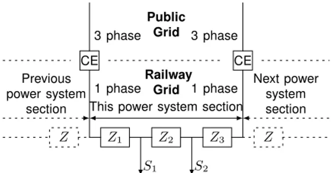
In this paper, like in [2], it is assumed that RPSSs can be divided into so-called power sections, whose borders are defined by so-called Connecting Equip-ment (CE). CE is a general term for where the RPSS is connected to the public grid. A deeper explanation why this assumption is valid can be found in [2].

Since all systems in this particular study are double-fed, this means that there is one converter station located in the beginning and one at the end of the power section. The term "double-fed" means here that a contact line is fed with electric power from not just one of its ends, but from both.

B. Binary Inputs

Like in [2], the approximator have two binary inputs determining the RPSS technology used – ̺ that attains value 1 when the catenaries are of AT (autotrans-former) type and 0 when they are not, and and η that is valued 1 when the RPSS is equipped with a supporting HV (high voltage) transmission line.

Sometime AT catenary systems [10]–[13] are also called dual systems or 2xVL kV systems (where VL denotes the voltage level) [12]. In the numerical exam-ples, a Sweden-inspired 16.7 Hz RPSSs are studied. Therefore, the cases where AT is not present are denoted BT (Booster Transformer) systems [10], [11], [13]. However, for 50 Hz RPSSs, one can simply consider it as a standard catenary system. This classi-fication of two kind of catenary technologies comprises also DC-fed RPSSs. There exist power-electronics based solutions with dual voltage contact line systems for DC railways [14].

C. Continuous Inputs

The remaining approximator inputs are, as in [2], in-puts to a neural network. One individual neural network is used for each RPSS technology, as illustrated in Figure 1. Why this separation is done is well explained in [2]. In this paper, however, the number of inputs is reduced to two, the most needed ones, i.e. the

S e le c to r TPSA outputs TPSA inputs AT ̺catenary HV η Remaining inputs TPSA NN #1 AT NN #2 AT+HV NN #3 BT NN #4 BT+HV

Fig. 1: For AT and BT (no AT) contact line types, which can be connected to an HV transmission line, there are four separate possible neural networks.

power section length and the number of trains in the power section. The power section lengths are numbers that the investment planner actively and directly can influence by choosing where to locate the CE. The longer a power section, the higher the impedance – regarding that everything else remains the same. A 100 km power section with AT catenaries have, on the other hand, for example, normally a higher impedance than a 110 km power section with AT technology and a supporting transmission line connected in parallel to it. The greater the number of trains, the higher the strain.

D. Output(s)

There are two alternative models for the output. The main model, Type A, similar to the one in [2], is the maximal possible on-average velocity of the trains in the section. The alternative output, Type B, represents instead the fastest travel-through time. In reality train traffic is much more complicated. However this is still a valid measure of the power system capacity limitations. For deeper discussions about neural networks and train traffic limitations, c.f. [2].

The number of TPSA neural network inputs are here limited on two inputs. This has eased the design of the neural networks such that their usability can be checked by common sense reality checks. Without considering possible traffic in other speed, and various slopes of the railway tracks we can isolate the causes of voltage drops to heavy traffic, and weak RPSS – no more no less. It will in the numerical examples of Sec-tion V also be shown that in most cases single-layered neural networks will perform well for approximating train velocities. In some cases two neuron layers were needed. In model Type B, with traveling time as TPSA output – often linear transfer functions [15] performed better than tansig transfer functions [15].

E. Discussion and Possible Future Improvements One possible drawback with traveling time as a possible optimization problem constraint instead of average velocities is that there would be no obvious upper bound in the former case, whereas in the latter the speed limit (physical or regulated) is an obvious upper bound. It is normally convenient to bound the solution space in great optimization problems.

The model presented in this paper is a simplified model, and discussions about how to instead extend the existing models to be more general can be found in e.g. [1], [2], [9].

A possible way of improving the simple and appli-cable TPSA version presented in this paper would be to put extra constraints on the neural networks. At the moment, simply the approximation error of the training data is made small with some extra convergence cri-teria. Assume however, that some measurements are more important than others. That could be considered in the design of an approximator. Moreover, assume, like in this case, that one knows things of the behavior of the function to approximate that maybe not the data set reflect perfectly. In this case, it is obvious that the partial derivatives of the traffic intensity as well as of the power section length should be negative if velocity is output, and conversely positive if traveling time is output. Since TPSA is designed to be used as optimization constraints, maybe even constraints of the sign of the second derivative in relevant domains may be of interest.

IV. Numerical Example Prerequisites A. Training of the Neural Networks

The aggregated input and output data sets are nor-malized to lie in the interval[−1, 1] by simple scaling before training and testing the approximators.

Training is essentially a method of determining the values of the neural network parameters (weights and biases) such that the network behaves as desired. Commonly, this means that the mean square of the estimation error of the network output is made small, which is the case also here.

In all, except one of the cases, the neural networks were trained by the trainbr (Bayesian regularization backpropagation [16]) algorithm (of Matlab’s Neural Network Toolbox). In the pure BT catenary RPSS, with traveling time as output, Type B, the training algorithm trainlm (Levenberg-Marquardt backprop-agation [17]) suited best to training data and desired function behavior. In many of the cases, with the specific simulation data used, trainlm tends to over-learn the presented data rather than extracting the important trends from it.

Normally, tansig transfer functions have been used for one hidden neuron layer with one neuron. In the RPSS with HV transmission line and AT catenaries, for train speed as output, i.e. Type A, two neurons in the hidden layer were needed to obtain satisfactory results. Other exceptions are the networks for all RPSS but the pure BT catenary system with traveling time as output, Type B, where the transfer functions are linear. For linear neural networks, there is no need for hidden layers – a linear function of a linear function can be rewritten as another linear function.

B. The Used Training Data

1) Introduction: The training data used for TPSA in this example are extracted out of TPSS [1], [18] simulations. The same models as in [18] with the exception that the filter in the motor is disregarded. The simulations represent variations in traffic, length, and the power system technology of a typical Swedish RPSS section.

However, the training data could as well have been created from measurements and be representing dif-ferent types of railway power systems than the one used here. Z Z1 Z2 Z3 Z S1 S2 1 phase CE 3 phase 1 phase CE 3 phase Previous power system

section This power system section

Next power system section Public Grid Railway Grid

Fig. 2: A section of the RPSS (railway power supply system), illustrated as an electric circuit.

As a consequence of the Swedish-like model, the CEs, c.f. Figure 2, are here converter stations, and the high voltage line is of the in Sweden most common 132 kV type. Contact lines and transmission lines are in Figure 2 represented by impedances.

2) Power System Infrastructure Used: In the simu-lations, each power section has the same contact line technology type (AT or BT, respectively) all over it, a consequence of the TPSA modeling. The simulated traffic is unidirectional.

In the Swedish railway power supply system, the defacto nominal contact line voltage level is 16.5 kV, however it is officially said to be a 10 % over voltage in a 15 kV system. The voltage angles at the converter station terminals are completely determined (although

quite nonlinearly) by the voltage levels, and the active and reactive power flows in and out (if possible and allowed) of the terminals of the converter station [19]. And converter stations are injecting more power to the railway, the more installed power there is in the station compared to its neighboring stations.

The converter stations, the CEs in Figure 2, at both ends of each power system section are in the simu-lations equipped with 6 10 MVA converters (Q48/Q49 [19]) each, i.e. 120 MVA in total. In some of the heavier trafficked situations simulated, the converter stations are overloaded. This is also a common case in real-life. However, the overloading of converter stations does not seem to be a cause of non-reliable solutions when the RPSS is heavily utilized. Tests have been made in such cases with 10 converters in each station with the non-reliability still there. Therefore, one can expect these situations be hard to find by other reasons, like e.g. great voltage drops or great changes in state values from one time-step to another.

It is here worth pointing out that in [1] it has been shown that the train velocities are in practice not dependent on the mutual distributions of apparent power capacity between a pair of converter stations, so these simulation results used for creating the training data are representative for all different variations of converter station capacities.

In the simulations with an HV transmission line present, the number of transformers connecting the transmission line to the contact line is set to three in all cases studied. This means that there are five transformers in total, three out on the track, and one connected to each converter station. The transformers are evenly distributed along the track.

3) Information About Trains Used: Since the model presented in Section III assumed only one kind of trains, the simulations used one kind of trains as well – Rc4 [20] in this case.

The speed-limit on the simulated track is in the simulations set as high as 150 km/h. That speed is for Rc4 locomotives a limiting constraint only in very steep downhill situations. All trains try to go as fast as possible in the TPSS simulations, i.e., as fast as the track speed-limits and the physical constraints of the railway in total allows. In the simulations used for creating the TPSA training data, the maximal-tractive-force curves from [20] was used. Exactly how they are used is explained in [18].

4) Description of Training Data Before Aggregation: For a detailed example about how TPSS output data might look, c.f. [1], [2].

In the simulations done, in contrast to in [2], all trains are traveling at 133 km/h (or the speed limit if the speed limit is lower than 133 km/h) when they

appear in the simulation. And they do not stop when leaving the power section, i.e. the speed is the high-est possible the train can have at that moment and location, considering legal, electrical and mechanical speed limitations. In other words, trains crosses the power section borders at full steam. This arrangement ensures that, in the simulation results, a longer power section (i.e. a weaker power system) should never result in a higher on-average train speed than a shorter one. The initial speed chosen reflects the steady-state speed when there are no voltage drops. To simulate accelerations and braking would, in a simplified ap-proximation like this one, result in a disfavor for shorter power sections since the train would not have time to reach full speed.

One smaller disadvantage with the in the above paragraph described arrangement is that for short power sections, the lowest train speed does not occur in the middle of the line – which would be the natural since the voltage is the lowest there. Instead it occurs closer to the end of the section.

In order to save TPSS computation time when simu-lating a certain headway of the traffic, trains are, at the beginning of the simulation, evenly distributed along the track assuming that the trains have been going at maximally allowed speed all the time – disregarding possible slopes, air resistances, or weaknesses in the power supply. These trains are so to say, the initial condition of the simulation.

In the initial conditions, the distributed trains, as-sumed to already be in traffic, have velocities set to the minimal value of 133 km/h and the speed limit. This is similar to the definitions of train speeds when entering the power section. After the simulation has started however, the trains distributed along the track with predefined initial velocities will follow the same electrical and mechanical laws of nature as the other trains.

In the numerical example, many different simulated situations have been used for each neural network to train. There are four separate neural networks for output Type A as well as for Type B. These fore make up; one for BT-type contact lines, one for AT-type contact lines, one for BT with HV transmission line, and finally one for AT with HV transmission line – as described in Figure 1.

The simulations are done on power sections with variable lengths, and train traffic headways. The head-ways span from 1 minute per train, up to 40 minutes per train, whereas the power section lengths vary from 25 km up to 300 km. This great span will sometimes imply very strong, and sometimes very weak RPSSs – depending of the technologies used. The different lengths and headways used for BT catenaries are

listed in Table I, where an ’X’ denotes a simulation has been done and that its aggregated results are used as training data for TPSA. The cases not studied depends normally on that TPSS has problems finding reliable solutions for each time step in these cases. Over the four Tables I-IV, the power section lengths studied may vary somewhat. That is an adaptation to where the last "nice and smooth" simulation results were extractable for a given headway. In all simulations, flat ground was assumed. The simulated cases for an AT RPSS are visualized in Table II, the cases for BT with HV transmission line in Table III, and cases for AT catenaries with supporting HV transmission line in Table IV. Some of the case studies create significant voltage drops and some not – the idea is to obtain varying results.

For the approximators with train average velocity as output, i.e. Type A, additive zeros were needed in order to make the approximator functions continuing decreasing after the lowest output measurement. It seems to be hard for TPSA to catch the strictly decreasing behavior of the trains maximal velocities for increased numbers of trains and increased power section lengths. Without this additive data, the TPSA function surfaces tended to flatten out to be constant at significant speeds for increased input data. It is important when keeping in mind that TPSA should be used as an optimization constraint that situations that are undesired or not even realizable in practice should be handled somehow. The undesired situations are, thanks to the added zeros, punished in such a way that they should not occur in the optimal solutions and that the constraint will be smooth and differentiable close to the expected possible future solutions. The added data varies in location, but is always 5 data points, far out from the measurements. The exact location is picked by hand, and considered satisfactory if it ensures negative trends of the output function for increasing values of the inputs – without increasing the approximation errors of the measurements.

For RPSS:s with AT catenaries, both with and with-out the HV line, it says that the maximal velocity of the trains should be 0 km/h when there are 140 trains on the power section and its lengths are 600 km, 650 km, and 700 km respectively. Moreover, for 700 km power sections, the maximal velocity is 0 km/h also when there are 130 and 135 trains in traffic. The correspond-ing zero-valued data for an RPSS with BT catenaries and not HV lines are 50 trains and power section lengths of 400 km, 450 km, and 500 km, respectively. Also for 500 km power sections, there is training data for 40 and 45 trains. In the case of BT catenaries with HV lines, zero speeds are added for power section distances 500 km – with 80, 85, and 90 trains

TABLE I: A summary of cases simulated for BT catenaries. Rows represent headways in minutes, columns power section lengths in km. A cross represents a simulated case, no cross mean that no simulation has been done

A summary of cases simulated for BT catenaries.

- 25 50 70 80 110 130 150 200 250 300 1 X X 2 X X X 3 X X X X 5 X X X X X 7 X X X X X X 10 X X X X X X X 20 X X X X X X X X 30 X X X X X X X X X 40 X X X X X X X X X X

TABLE II: A summary of cases simulated for AT catenaries. Rows represent headways in minutes, columns power section lengths in km. A cross represents a simulated case, no cross mean that no simulation has been done

A summary of cases simulated for AT catenaries.

- 25 50 70 80 110 130 160 200 260 300 1 X X X X X X 2 X X X X X X X 3 X X X X X X X X 5 X X X X X X X X X 7 X X X X X X X X X X 10 X X X X X X X X X X 20 X X X X X X X X X X 30 X X X X X X X X X X 40 X X X X X X X X X X

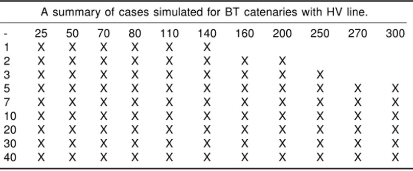
TABLE III: A summary of cases simulated for BT catenaries and HV transmission line. Rows represent headways in minutes, columns power section lengths in km. A cross represents a simulated case, no cross mean that no simulation has been done

A summary of cases simulated for BT catenaries with HV line. - 25 50 70 80 110 140 160 200 250 270 300 1 X X X X X X 2 X X X X X X X X 3 X X X X X X X X X 5 X X X X X X X X X X X 7 X X X X X X X X X X X 10 X X X X X X X X X X X 20 X X X X X X X X X X X 30 X X X X X X X X X X X 40 X X X X X X X X X X X

respectively; 450 km with 90 trains, and 400 km with 90 trains. The five extra points for BT catenaries can be seen to the right in Figures 5a and 5b in the results section.

V. Numerical Results Visualized

Two different outputs have been evaluated for TPSA, with more emphasis on the average velocity, Type A. Type A have been studied earlier in [2], [6]. The traveling time as output has however some po-tential and is worth being evaluated in real investment

analysis programs before rejected.

For both of the outputs, TPSA is evaluated for input values far away from the training data, and from what is realistic in reality. If, however, TPSA is supposed to be used as an optimization constraint, it is important to know how it behaves also for values far away. For the rare occasions, where e.g., TPSA gives velocity estimates less than zero those can be handled by simply assigning zero velocity then.

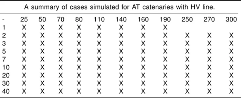
TABLE IV: A summary of cases simulated for AT catenaries and HV transmission line. Rows represent headways in minutes, columns power section lengths in km. A cross represents a simulated case, no cross mean that no simulation has been done

A summary of cases simulated for AT catenaries with HV line. - 25 50 70 80 110 140 160 190 250 270 300 1 X X X X X X X X 2 X X X X X X X X X X X 3 X X X X X X X X X X X 5 X X X X X X X X X X X 7 X X X X X X X X X X X 10 X X X X X X X X X X X 20 X X X X X X X X X X X 30 X X X X X X X X X X X 40 X X X X X X X X X X X

A. Average Velocity as Output – Type A

The designs of the neural networks were not de-termined in any systematical way, but designed such that a combination of small approximation error to measurements and added data points, and of a func-tion behavior in correspondence to experience and engineering common sense was obtained.

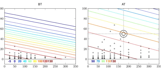
In Figure 3, TPSA interpolates and extrapolates the maximal average train velocities as functions of power section lengths and number of trains for four different power system types. As one can expect, and as the figures confirm, the pure BT system is the one that drops in maximal train velocity the fastest, and the AT system with HV transmission line the toughest RPSS type. for an increased number of trains on a section. This is visualized in a clearer, and more detailed way, by subtracting the average velocity of one system from another in Figure 4.

To further clarify how Figure 3 should be interpreted, in subplot Figure 3b, some extra circles and lines have been added. First of all, the circles and the crossing of the line in Figure 3b marks out a spot where there are 50 trains on a 175 km long power section. According to the contours, the legend, and the caption text, trains there could go in slightly more than 110 km/h. Moreover, one can see that the added dotted lines split the plot into four parts. In the lower left part of the plot, there are lots of simulation data located. There, TPSA mainly interpolates to measurements. In the upper left, and the lower right parts of the figure, the measurements are fewer, so here TPSA extrapolates to a great extent. Finally, in the upper part of the figure, TPSA extrapolates mainly. Con-sidering the added zeros outside the figure, around 700 km and 140 trains, c.f. Section IV-B4, there is a bit interpolation being done also. In the areas where TPSA extrapolates, naturally, the uncertainty of the estimated values are greater, and there TPSA should

not be used primarily as a designing tool. These extrapolated areas are however needed to exist, be easily differentiable, and to make sure that the output values are worse off for weaker and for more strained power systems. If not, there would be a risk that an optimization program, using TPSA as a constraint would find optimal solutions where the power system in reality would be very strained.

Finally, it is time to study the approximation er-rors for TPSA. In Figure 5, one can see that the maximal overestimation of train velocity is 8.7 km/h and that the maximal underestimation of train velocity is 5.0 km/h. This must be considered a reasonable solution considering the simplicity of the approximator and the applicative purpose of the approximator. The interpretation of each circle in Figure 5 is clarified by an example: The uppermost circle is located at 5, i.e. the approximation is an underestimation of 5 km/h. Looking at Figure 5a one can see that this point represent a simulation that has been done for 25 trains within the power section. Looking at the same time at Figure 5b one also see that this point represent a 50 km long power section.

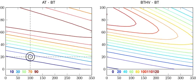
1) Illustrations of the Value of RPSS investments: A clarification similar to the one of how to interpret Figure 3 follows for Figure 4 follows. Consider the circles and intersecting dashed lines in Figure 4a. In the point indicated by the cross and the circles, for 100 km/h power section, and 20 trains, an RPSS infrastructure upgrade from BT catenaries to AT catenaries would result in a gain of slightly less than 20 km/h in average speeds. Considering the huge voltage drops on BT catenaries, the speed gains by an investment further up or to the right from this point on in the plot will be less reliable down to the last digit, c.f. with the same spot in Figure 3a. It will however be quite clear, that if a gain of 30 km/h or more is estimated for a BT-to-AT upgrade in a given hypothetic situation, it is obvious that some kind of upgrade should already have been

-5 0 20 40 60 80100120130 0 50 100 150 200 250 300 350 0 20 40 60 80 100 BT

(a) BT-type contact lines and no HV transmission lines. The upper-most curve represents -5 km/h, the next one 0 km/h, thereafter every tenth km/h until 130 km/h. 50 70 90110130 0 50 100 150 200 250 300 350 0 20 40 60 80 100 AT

(b) AT-type contact lines and no HV transmission lines. The up-permost curve represents 50 km/h, thereafter every tenth km/h until 130 km/h. 10 30 50 70 90110130 0 50 100 150 200 250 300 350 0 20 40 60 80 100 BTHV

(c) BT-type contact lines with HV transmission lines. The uppermost curve represents 10 km/h, thereafter every tenth km/h until 130 km/h.

90110130 0 50 100 150 200 250 300 350 0 20 40 60 80 100 ATHV

(d) AT-type contact lines with HV transmission lines. The uppermost curve represents 90 km/h, thereafter every tenth km/h until 130 km/h.

Fig. 3: Contour plots of how TPSA estimates the train velocity differences for given RPSS type, power section length, and number of trains. Text in various colors represent different train velocities in km/h. Horizontal axis represents km length of the power section, whereas vertical axis represents the number of trains in the section. The locations of the training data obtained through simulations are marked by black pluses.

done.

One can in Figure 4a see, that AT technology with this model always outperforms BT technology. The approximator for AT technology with HV transmission line, quite naturally represents the far strongest RPSS, as can be seen when the AT approximator, c.f. Figure 4c, and the BT with HV approximator, c.f. Figure 4d, respectively, are subtracted from it.

B. Traveling Time as Output – Type B

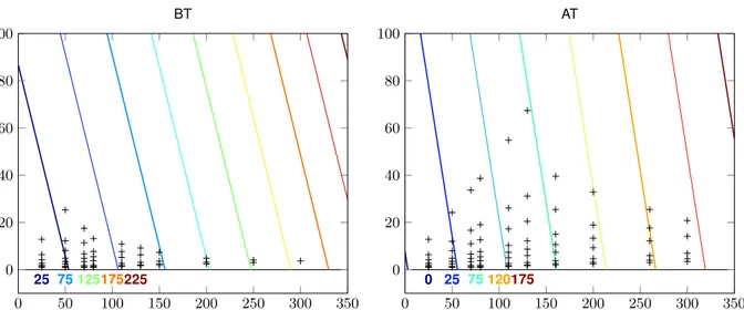
When traveling time is the output, the TPSA results are presented in Figure 6. The figure should be in-terpreted similarly to Figure 3, with the only exception that each curve represents a specific traveling time in minutes instead of an average speed. It is natural that the dependency here is much stronger for increased distance, because even for a slightly increased speed, the traveling times would increase for an increased distance to travel.

0 10 20 30 40 50 −10

−5 0 5

(a) Vertical axis represents the approximation errors in km/h, whereas the horizontal axis represents the number of trains in traffic in the power section.

0 100 200 300 400 500

−10 −5 0 5

(b) Vertical axis represents the approximation errors in km/h, whereas the horizontal axis represents the length of the power section in km.

Fig. 5: Plots of the approximation errors for TPSA with velocity output, representing a BT RPSS – the technology that resulted in the greatest approximation errors.

The approximation errors were, for the time output, the biggest for an RPSS with AT technology. These plots in Figure 7 should be interpreted analogously to Figure 5 with the main exception that the errors are in minutes instead of km/h.

VI. Conclusion, Summary, and Future Work A suggestion to an improved TPSA method, of estimating the power system impact on traffic perfor-mance, has been presented in Sections III and IV. The function approximator uses aggregated parametric values for inputs as well as for output. The proposed method is general in many ways. There are no indi-cations that TPSA should not be possible to apply to

0 10 20 30 40 50 60 70

0 5 10

(a) Vertical axis represents the approximation errors in minutes, whereas the horizontal axis represents the number of trains in traffic in the power section.

0 50 100 150 200 250 300

0 5 10

(b) Vertical axis represents the approximation errors in minutes, whereas the horizontal axis represents the length of the power section in km.

Fig. 7: Plots of the approximation errors for TPSA with traveling time output, representing an AT RPSS – the technology that resulted in the greatest approximation errors.

other kinds of doubly fed RPSS:s (including doubly fed DC RPSS:s), than those used in the numeric example. TPSA has been applied to a small specific railway power supply system in order to confirm its usability.

TPSA was evaluated in Section V, for both output Type A and B, but with emphasis put on Type A. In most Type A configurations one hidden neuron was enough, and in most Type B configurations linear neural networks performed well.

In order to visualize the behavior of an RPSS, and how TPSA manages to adapt, a number of graphs in Figures 3–7 were presented and their content was discussed in detail in Section V.

It is obvious that TPSA manages to give reliable results in a fast way for given power system setups and traffic intensities.

The results presented in this paper, show that by making many simulations (or detailed measurements) and studying the results – a feeling can be acquired for what is important regarding the railway power supply system and its interaction with the train traffic. Owing to that, the here presented approximator could be made. Improvements in TPSA can be made in the sense that for more all-embracing data sets, different inputs would be possible, see the discussions in Section III-E. Future work are naturally to apply TPSA in invest-ment decision programs, like in [6] but improved. TPSA can also be applied in traffic planning programs.

References

[1] L. Abrahamsson, “Railway Power Supply Models and Methods for Long-term Investment Analysis,” Royal Institute of Technology (KTH), Stockholm, Sweden, Tech. Rep., 2008, Licentiate Thesis. [Online]. Available: http://kth.diva-portal.org/ smash/get/diva2:117/FULLTEXT02

[2] L. Abrahamsson and L. Söder, “Fast Estimation of Relations between Aggregated Train Power System Data and Traffic Performance,” IEEE Journal of Vehicular Technology, vol. 60, no. 1, pp. 16–29, Jan. 2011. [Online]. Available: http: //ieeexplore.ieee.org/xpls/abs_all.jsp?arnumber=5624653 [3] J. v Lingen and P. Schmidt, “Railway Electric Energy Supply

and Operation of Railways (original title in German),” Elek-trische Bahnen, vol. 96, no. 1–2, pp. 15–23, 1998.

[4] S. Acikbas and M. T. Söylemez, “Coasting point optimisation for mass rail transit lines using artificial neural networks and genetic algorithms,” IET Electric Power Applications, vol. 2, no. 3, pp. 172–182, 2008.

[5] S. P. Gordon and D. G. Lehrer, “Coordinated train control and energy management control strategies,” in Railroad Confer-ence, 1998. Proceedings of the 1998 ASME/IEEE Joint, Apr. 1998, pp. 165–176.

[6] L. Abrahamsson and L. Söder, “Railway power supply invest-ment decisions considering the voltage drops - assuming the future traffic to be known,” in Intelligent System Applications to Power Systems, 2009. ISAP ’09. 15th International Conference on, 2009, pp. 1–6.

[7] T. A. Kneschke, “Simple method for determination of substation spacing for ac and dc electrification systems,” Industry Appli-cations, IEEE Transactions on, vol. IA-22, no. 4, pp. 763–780, 1986.

[8] S. Methner, “Multicriterial Optimization for Elecric Railway Sys-tems (original title in German),” Dresden University of Technol-ogy, Tech. Rep.

[9] L. Abrahamsson and L. Söder, “Fast estimation of the relation between aggregated train power system information and the power and energy converted,” in Universities Power Engineer-ing Conference, 2008. AUPEC ’08. Australasian, Dec. 2008, pp. 1–6.

[10] R. J. Hill, “Electric railway traction, Part 3 Traction power supplies,” Power Engineering Journal, vol. 8, no. 6, pp. 275– 286, Dec. 1994.

[11] A. Bülund, P. Deutschmann, and B. Lindahl, “Circuitry of overhead contact line network at swedish railway Banverket (original title in German),” Elektrische Bahnen, vol. 102, no. 4, pp. 184–194, 2004.

[12] E. Pilo, L. Ruoco, and A. Fernández, “A reduced representa-tion of 2x25kv electrical systems for high-speed railways,” in Proceedings of the 2003 IEEE/ASME Joint Rail Conference, Apr. 2003, pp. 199–205.

[13] J. D. Glover, A. Kusko, and S. M. Peeran, “Train Voltage Analysis for AC Railroad Electrification,” IEEE Transactions on Industry Applications, vol. IA-20, no. 4, pp. 925–934, Jul./Aug. 1984.

[14] P. Ladoux, F. Alvarez, G. J. Hervé Caron, and J.-P. Perret, “A new structure of power 1500V catenary: the system 2 x 1500 V (original title in French),” Revue Genérale des Chemins de Fer, vol. 21, pp. 21–31, 2006.

[15] S. Haykin, Neural Networks. Englewood Cliffs: Prentice Hall, 1999.

[16] “Neural network toolboxTM_{,” Jul. 2008, about the "trainbr"}

training algorithm. [Online]. Available: http://www.mathworks. com/access/helpdesk/help/toolbox/nnet/trainbr.html

[17] “Neural network toolboxTM_{,” Jul. 2008, about the "trainlm"}

training algorithm. [Online]. Available: http://www.mathworks. com/access/helpdesk/help/toolbox/nnet/trainlm.html

[18] B. Boullanger, “Modeling and simulation of future railways,” Master’s thesis, Royal Institute of Technology (KTH), Mar. 2009. [Online]. Available: http://www.kth.se/ees/forskning/ publikationer/modules/publications_polopoly/reports/2009/ XR-EE-ES_2009_003.pdf?l=en_UK

[19] H. Kols, “Frequency Converters for Railway Feeding (original title in Swedish),” Swedish national railway administration (Ban-verket), Tech. Rep. BVH 543.17000, May 2004.

[20] N. Jansson, “Electrical Data for the Locomotive Types Rc4 and Rc6 (original title in Swedish),” TrainTech, Solna, Tech. Rep., Mar. 2004.

10 30 50 70 90 0 50 100 150 200 250 300 350 0 20 40 60 80 100 AT - BT

(a) BT-type contact lines approximator subtracted from AT-type approximator. The uppermost curve represents 70 km/h, thereafter every tenth km/h until 90 km/h, whereafter it starts to fall, every tenth km/h down to 10 km/h. 0 20 40 60 80100110120 0 50 100 150 200 250 300 350 0 20 40 60 80 100 BTHV - BT

(b) BT-type contact lines approximator subtracted from BT-type approximator with HV transmission lines. The uppermost curve repre-sents 30 km/h, thereafter every tenth km/h until 110 km/h, whereafter it starts to fall, every tenth km/h down to 0 km/h. A glimpse of the curve for 120 km/h can also be seen.

0 20 40 0 50 100 150 200 250 300 350 0 20 40 60 80 100 ATHV - AT

(c) AT-type contact lines approximator subtracted from AT-type ap-proximator with HV transmission lines. The uppermost curve repre-sents 40 km/h, thereafter every tenth km/h until 0 km/h.

0 20 40 60 70 0 50 100 150 200 250 300 350 0 20 40 60 80 100 ATHV - BTHV

(d) BT-type contact lines with HV transmission line approximator subtracted from an AT-type contact line with HV transmission line approximator. The uppermost curve represents 70 km/h, thereafter every tenth km/h until 0 km/h.

Fig. 4: Contour plots of TPSA estimator differences, i.e. the gains in train speeds by investing in an RPSS reinforcement. Contours represent the train velocities for given RPSS type, power section length, and number of trains. Text in various colors represent different train velocities in km/h. Horizontal axis represents km length of the power section, whereas vertical axis represents the number of trains in the section.

25 75125175225 0 50 100 150 200 250 300 350 0 20 40 60 80 100 BT

(a) BT-type contact lines and no HV transmission lines. The rightmost curve represents 225 min., the next one 200 min., thereafter every twenty-fifth minute until 25 min.

0 25 75120175 0 50 100 150 200 250 300 350 0 20 40 60 80 100 AT

(b) AT-type contact lines and no HV transmission lines. The rightmost curve represents 175 min., thereafter every twenty-fifth minute until 0 min. 0 25 75120175 0 50 100 150 200 250 300 350 0 20 40 60 80 100 BTHV

(c) BT-type contact lines with HV transmission lines. The rightmost curve represents 175 min., thereafter every twenty-fifth minute until 0 min. 25 75125150 0 50 100 150 200 250 300 350 0 20 40 60 80 100 ATHV

(d) AT-type contact lines with HV transmission lines. The rightmost curve represents 150 min., thereafter every twenty-fifth minute until 25 min.

Fig. 6: Contour plots of how TPSA estimates the train traveling times for given RPSS type, power section length, and number of trains. Text in various colors represent different times in minutes. Horizontal axis represents km length of the power section, whereas vertical axis represents the number of trains in the section. The locations of the training data obtained through simulations are marked by black pluses.