Traffic noise effects of property prices: Hedonic estimates
based on multiple noise indicators
Henrik Andersson, Jan-Erik Swärdh & Mikael Ögren – VTI CTS Working Paper 2015:11
Abstract
Valuation of traffic noise abatement based on hedonic pricing models of the property market has traditionally measured the noise as the equivalent, or another average, level. What is not captured in such a noise indicator is the maximum noise level of a vehicle passage. In this study, we incorporate the maximum noise level in the hedonic model letting the property price depend on both the
equivalent noise level and the maximum noise level. Hedonic models for both rail and road noise are estimated.
Data consists of characteristics of sold properties, property-specific noise calculation, and geographical variables. We use the hedonic approach to estimate the marginal willingness to pay (WTP) for maximum noise abatement where we model the effect as the maximum noise level subtracted with the equivalent noise level. Furthermore, we control for the equivalent noise level in the estimations.
The estimated results show that including the maximum noise level in the model has influence on the property prices, but only for rail and not for road. This means that for road we cannot reject the hypothesis that WTP for noise abatement is based on the equivalent noise level only. For rail, on the other hand, we estimate the marginal WTP for the maximum noise level and it turns out to be substantial. Also, the marginal WTP for the equivalent noise levels seems to be unaffected by the inclusion of the maximum noise level in the model. More research of this novel topic is requested though.
Keywords: Noise, Hedonic regression; Rail, Road; Equivalent level; Maximum level JEL Codes: C21; C26; Q51; Q53
Centre for Transport Studies SE-100 44 Stockholm
Sweden
Traffic noise effects on property prices: Hedonic estimates
based on multiple noise indicators
∗Henrik Andersson
Toulouse School of Economics (UT1, CNRS, LERNA), France
Jan-Erik Swärdh†
Department of Transport Economics, VTI, Sweden Mikael Ögren
Sahlgrenska University Hospital, University of Gothenburg, Sweden June 30, 2015
Abstract
Valuation of traffic noise abatement based on hedonic pricing models of the property market has traditionally measured the noise as the equivalent, or another average, level. What is not captured in such a noise indicator is the maximum noise level of a vehicle passage. In this study, we incorporate the maximum noise level in the hedonic model letting the property price depend on both the equivalent noise level and the maximum noise level. Hedonic models for both rail and road noise are estimated.
Data consists of characteristics of sold properties, property-specific noise calculation, and geo-graphical variables. We use the hedonic approach to estimate the marginal willingness to pay (WTP) for maximum noise abatement where we model the effect as the maximum noise level subtracted with the equivalent noise level. Furthermore, we control for the equivalent noise level in the estimations. The estimated results show that including the maximum noise level in the model has influence on the property prices, but only for rail and not for road. This means that for road we cannot reject the hypothesis that WTP for noise abatement is based on the equivalent noise level only. For rail, on the other hand, we estimate the marginal WTP for the maximum noise level and it turns out to be substantial. Also, the marginal WTP for the equivalent noise levels seems to be unaffected by the inclusion of the maximum noise level in the model. More research of this novel topic is requested though.
Keywords: Noise, Hedonic regression; Rail, Road; Equivalent level; Maximum level JEL Codes: C21; C26; Q51; Q53
∗This study was funded by the Swedish Transport Administration, and the financial support is gratefully acknowledged.
Comments and suggestions by Mats Wilhelmsson and participants of the seminar at VTI Stockholm 19th of November 2014 are appreciated. The authors are solely responsible for the paper.
†To whom correspondence should be addressed: VTI, Box 55685, SE-102 15 Stockholm, Sweden. E-mail:
1
Introduction
The society costs of traffic noise are external costs that follow from the utilization of the traffic system. Such types of external costs are to be included in cost-benefit analysis (CBA) of investments and measures in the transport sector. Also, increased urbanization may worsen the problems with traffic noise over time.
To include noise costs in CBA we need to have estimates of individuals’ willingness to pay (WTP) for traffic noise abatements. Essentially there are two strategies to come up with such WTP estimates of goods that are not directly purchased in the market.
The common strategies to valuate non-market goods, such as noise, are to use either individuals’ actual choices of another market or direct choices of hypothetical scenarios. Indirect analyses of another real market are usually termed revealed preference (RP) analysis while hypothetical experiments usually is termed stated preference (SP) analysis. Both methods have been relatively frequently used for noise valuation. RP studies of noise valuation is mostly based on the hedonic model (Rosen, 1974). The price of goods with different characteristics, which different individual place different values to, is analyzed by the hedonic model (see e.g. Sheppard, 1999). Such a market consists of goods that are close substitutes, i.e. satisfy the same need, but where the different characteristics reflects the price. Private properties are such a substitutable good and the housing market is one of the most studied markets in the hedonic literature. Nelson (2008) describes comprehensively the hedonic framework of noise valuation with a review of the literature and a focus on challenges for the future. Regarding SP-studies, on the other hand, Bristow et al. (2015) is a comprehensive study that summarize 258 noise valuations from 49 different studies within the meta-study framework. There is a lot of evidence for the noise valuation to differ with respect to e.g. noise source and noise level (Bristow et al., 2015).
What is less focused on in the literature, however, is the effect of different noise measures and how they can be used in CBA. Most studies use the equivalent noise level which is a weighted average of the noise exposure over a given time period, usually a 24-hour period. Nonetheless, to estimate the WTP for noise abatement where noise is measured by the equivalent level may not capture all negative effects of traffic noise exposure. Instead, there may be occasions of noise exposure where the equivalent noise level does not approximate noise annoyance sufficiently. Low traffic and living really close
to the noise source may be examples in this aspect. The maximum noise level and the number of noise events may thus also be important for the WTP of noise abatement. This is policy relevant because there might be more disutilities from noise exposure that is not captured by the equivalent noise level, which may be especially important where the traffic flow is relatively low meaning that you have a low equivalent noise level but still is disturbed by the few noise events close to your property. Then the valuation input to CBA may be wrong potentially leading to inefficient resource allocation.
Baranzini and Ramirez (2005) use more than one single noise measure in the hedonic estimation of apartment rents in Geneva, Switzerland. Except some kind of average
noise measures, they also use dynamic noise in their estimations. Dynamic noise is
defined as the peak noise level, i.e. the noise level that is exceeded 10 percent of the time, subtracted with the background noise level. Also, the noise pollution level defined as the sum of average noise and dynamic noise is used in the estimation. Note however that Baranzini and Ramirez (2005) use measured overall noise and do not distinguish between different noise sources. The results show that the total impact of noise is fundamentally the same, whatever noise measure used (Baranzini and Ramirez, 2005).
The objective of this study is to estimate the WTP of traffic noise where noise is measured both by the equivalent level and the maximum level. As far as the authors know, there is no hedonic valuation study analyzing the simultaneous effect of both these noise measures, although the approach of Baranzini and Ramirez (2005) is relatively closely related. The analysis of Baranzini and Ramirez (2005) is in our study extended in a number of different ways. First, although calculated by admitted methods, our noise indicators are due to specific traffic noise sources as road traffic and rail traffic whereas Baranzini and Ramirez (2005) use the overall noise and are thus not able to distinguish
between different noise sources. This means that our results can be used for policy
purpose, for example in CBA of investments and measures within the transport sector, of specific traffic modes. Furthermore, in our study we calculate the maximum noise level which is not the peak level as used in Baranzini and Ramirez (2005). Especially regarding rail traffic, both these mentioned distinctions may be important as the maximum noise level of these separate noise events can be important for the disutility and thus capitalized into the housing market.
The hedonic approach is used in this study and, also, the representation of noise turns out to not significantly influence the noise valuation in the meta-study of Bristow et al.
(2015). Nevertheless, concerns about the chosen method have to be made.
Firstly, we will discuss how multiple noise measures can be included in CBA, mostly with focus on substitutable or complementary noise effects. To implement a single noise measure in CBA can be complex and this is a hint to us about the complexity of imple-menting more than one noise measure. There are essentially two strategies to incorporate the maximum noise effect in CBA. First, the WTP for noise abatement can be a function of both the equivalent noise level and the maximum noise level. The other strategy at hand would be to model the property price as a function of the maximum noise level only and calculate WTP estimates based on maximum noise that can be used as a substitute to WTP estimates based on equivalent noise. The main problem with the latter approach is that it will be arbitrary which model to use in a particular situation. If some criteria would be determined, it is not clear what these criteria should be and how they should be determined. There is also a risk that such substitutable models are used in favor of an underlying objective. With this features in our mind, we argue for the first approach. Note however, that if the total noise cost is approximately the same regardless of the noise measures used as in Baranzini and Ramirez (2005), separate noise effects would be complementary but do not on the aggregate level change the total cost of noise pollution. Still, there might be occasions where the separate effects are needed to better capture the noise annoyance. We will present relevant policy use examples of this issue in the Discussion section of the paper.
Secondly, we will also pay attention to valuation based on the hedonic model and its limitation. The estimated noise values are based on what is priced into the housing market and therefore it is necessary that the disutilities are observed by the property buyers.
Thirdly, here follows also the important issue of health effects vs. disturbance effects. Maximum noise levels may be most important for sleep disturbances, which we do not know whether they are included in hedonic model based valuations.
Finally, there is a brief discussion about alternative methods for analyzing the disutility effect of maximum noise levels.
The rest of the paper is outlined as follows. In Section 2, we describe our data and present descriptive statistics. The empirical framework is described in Section 3 followed by the estimated results in Section 4. The paper is finalized with a discussion including implementation of the results, and conclusions in Sections 5 and 6.
2
Data
In this study we use data of four different Swedish regions.1 The regions are Falköping,
Hässleholm, Borås, and Falun. Falköping and Hässleholm are used for analyses of rail noise while Borås and Falun are used for analyses of road noise.
In Table 1, characteristics of these regions are presented.
For this study we have chosen rail regions with more than one railway line for variation of the maximum level. For road the choice was dependent on the possibilities to calculate the maximum noise level.
2.1 Property data
Data of all property sales involving only private people in our municipalities from autumn of 1996 to 2010 regarding rail noise and from 2002 to August 2012 regarding road noise are recorded. Although observed over time, we treat data as cross-sectional, and we therefore include the latest observed sale of each property.
We are using property price, living space, subsidiary space, property area, age of dwelling, quality index, linked house, terraced house, bordering a sea or lake, and taxation value as the information taken from the property sales register.
Included are only sales between private individuals. When a municipality authority is selling a property it can be subsidized with the reason to attract tax-payers to the municipality and we want to exclude such interventions of the market.
The property prices are deflated to the prices of 2009. County-specific yearly indices of property prices are used for deflation. Since the prices of housing markets can develop differently for municipalities within a county, we also use yearly indicator variables in the estimations of the hedonic model.
1We prefer to use the term region, note however that they are consisting the Swedish administrative classification of
T able 1: Description of the m u nicipalities Municipalit y P opulation Lo cal Railw a y lines Closest Re gional lab or urban cen ter mark et area cen ter (y e s/no) F alk öping 31 974 Sk ö vde Västra Stam banan Gothen burg (108 km) No Jönk öpingsbanan Hässleholm 50 214 Kristianstad Sö dra Stam banan Malmö (78 km) No Skånebanan Mark arydsbanan Borås 105 783 Gothen burg -G o the n burg (56 km) No F alun 56 772 F alun-Borlänge -Sto ckholm (196 k m ) Y es Notes : Lo cal lab or mark ets are defined b y Statistics Sw eden based on comm uting flo w s b et w een m unicipalities. P opulation data is from No v em b er 1st of 201 3.
Geographical variables are calculated with the aim to capture accessibility effects and/or exposure effects other than noise. The variables we use are distance to railway station, distance to railway and distance to road. Distance to railway station captures accessibility effects and thus distance to railway is expected to capture other possible (negative) effects of living close to the railway. Distance to road capture both positive accessibility effects and negative effects other than road noise such as barrier effects and pollution. Hence, the expected sign of distance to road is ambiguous. Given from prop-erty data are also geographical areas within each region, which are used as indicator variable controls in our hedonic models.
2.2 Noise data
For the four regions in the study the equivalent noise levels were calculated in previous studies (Swärdh et al., 2012; Andersson et al., 2013). The maximum noise levels were then calculated using the standard Nordic prediction methods for rail (Ringheim, 1996) and road (Jonasson and Nielsen, 1996) traffic noise. In both cases the same limitations as in the previous studies apply, mainly that shielding by buildings is taken into account using a simplified procedure when many detached houses are grouped together, and that only major noise barriers are included. The terrain heights, road and railway positions and posted speeds were obtained exactly in the same way as in the previous studies.
For railway traffic the maximum length of freight trains is of importance to the max-imum level, and it was assumed that no freight trains were longer than 750 meters. Passenger trains were assumed to have their standard lengths. Maximum levels were cal-culated for all train types for each location, and the final maximum level is the maximum of all train types. Typically the maximum level is determined by freight trains where the speeds are low and high speed trains where the posted speed limit is high, at least for short distances between the railway and the receiver.
For road traffic the maximum level is determined by the heavy vehicles unless there are no heavy vehicles at all on the road closest to the receiver. Several different ways of determining the maximum level are in use for road traffic noise, but here we used the original definition from section 3 in Jonasson and Nielsen (1996). Note that there is a correction under 3.4 in the method that stipulates that the calculated maximum level can never be lower than the equivalent level, which we have applied.
seen as limiting although changes in traffic volume over time have to be very large for influencing the noise levels substantially. For road noise, traffic data of 2010 is used and for rail noise, traffic data of 2008 is used.
2.3 Estimation sample
The samples are restricted in some different ways to be suitable for hedonic analysis. First we aim to restrict the sample to include properties that may experience noise disturbances. Here, we believe that basing this restriction on noise levels is inflexible, especially when we also valuate maximum noise. Instead the basis of the restriction is on distance to railway or distance to road. In particular, the rail data includes properties closer than 1000 meters from the railway. For road, only properties within 150 meters from the closest road are included. This may be seen as a large difference between roads and railways but roads are distributed in a network where few properties are located far away from a road. Railways are, on the other hand, lines where you do not are exposed to railway noise if you are located far away from this railway line. As will be seen, there is still a higher mean level of the equivalent noise in the rail sample so this restrictions will probably not cause any systematic differences. In addition, the latter is consistent with the experience that maximum noise is a problem mostly for individuals living in properties close to the road.
Furthermore, we exclude properties with respect to living space and property area. If living space exceeds 505 square meters or is less than 31 square meters, the property is excluded. The same holds for property areas of 10 000 square meters or above. The argument for those restrictions is that we want data with properties used purely as private residences and by including these outliers we may include other type of properties. In addition, the noise is calculated at the center of each property and with large property areas the dwelling can be located considerably far away from the center.
In addition, the regions will be pooled in the hedonic analysis. This is a simplification that we will test in the sensitivity analysis of Section 4. The reason for pooling is to incorporate sufficient variation in all of the noise variables, which we aim for by including more than one region in the same estimation. In addition, spatial consideration is taken into account through geographical area indicators in the models but we will use OLS as the estimation procedure. OLS is a consistent alternative to a spatial error model (Anselin, 1999) and regarding the spatial lag model it is unclear whether the indirect
term should be included in the implicit price (Small and Steimetz, 2012).2
Further, we annualize all property prices before estimation by multiplying the property prices with
0.0311 + 0.01τi Pi
. (1)
In this expression, 0.0311 captures the long-term real interest rate on housing loans, which is based on the weighting average ten-year nominal interest rate in 2009 equal to
5.11 percent3 minus the 2 percent inflation objective of the Central Bank of Sweden,
which we assumed is the expected inflation rate. Note that the price year of our study is set to 2009. τ is the property-specific taxation value which is taxed with 1 percent of its value per year for most of our observation years4.
2.4 Descriptive statistics
In Tables 2 and 3, descriptive statistics for the noise variables equivalent noise level (Leq),
maximum noise level (Lmax), and DIFF (Ldiff) is presented. DIFF is the variable where
the maximum noise level is subtracted by the equivalent noise level, i.e. Ldiff = Lmax−Leq.
First in Table 2 we present mean and standard deviation of the noise variables. The results are presented for each region separately but also for the rail regions and road regions together. Recall that to be included a distance to railway below 1000 meters is required. If we compare the different regions we can see that they are relatively similar. The main difference is that the noise variables seem to be higher in Hässleholm than in Falköping. Also, the variation of the noise variables is larger in Hässleholm than in Falköping. This particularly holds for the Lmax and the Ldiff.
For road we can see a number of differences compared to the rail data. First, both
Leq and Lmax have a much lower mean value for road. Furthermore, Ldiff has a very
similar mean for road as for rail. However, there is much more variation in Ldiff for road
compared to rail. The reason is that the more continuous traffic flow of roads implies
that Ldiff can take much lower values for road than for rail. Some properties even have
a zero modeled difference between Lmax and Leq.
2We have tested spatial error models by using Stata and due to calculation problems we estimated the model on a
random sample of 900 properties for rail and road respectively. The results are very similar to corresponding OLS models and in fact the spatial component is not statistically significant for road.
3Holds for Swedbank, which is one of the largest providers of housing loans in Sweden and also provides data of
historic interest rates on their web page, see http://hypotek.swedbank.se/rantor/historiska-rantor/historik-bostadsrantor-2008-2009.
4This is a simplification, see the discussion in the previous working papers Swärdh et al. (2012) and Andersson et al.
T able 2: Descriptiv e statistics of railw a y noise v ariables Rail Road V ariable Both regions Hässleholm F alk öping Both regions Borås F alun Equiv alen t noise -Leq 53.3 53.0 53.7 47.0 47.0 47.0 (5.57) (5.80) (5.1 6) (6.51) (6.23) (6.95) Maxim um noise -Lmax 68.4 68.0 69.0 62.3 61.9 62.8 (7.90) (8.36) (7.0 8) (7.50) (7.51) (7.45) DIFF: Ldiff = Lmax − Leq 15.1 15.0 15.2 15.3 14.9 15.9 (3.18) (3.58) (2.4 1) (6.97) (6.86) (7.12) No of obs erv ations 2575 1572 1003 3783 2347 1436 Notes : Mean v alues with standard deviation in paren thesis. 2575 observ ations for rail and 3783 observ ations for road.
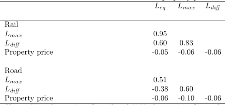
Table 3: Correlation of noise variables and property price Leq Lmax Ldiff Rail Lmax 0.95 Ldiff 0.60 0.83 Property price -0.05 -0.06 -0.06 Road Lmax 0.51 Ldiff -0.38 0.60 Property price -0.06 -0.10 -0.06
Notes: 2575 observations for rail and 3783 observations for road.
In the correlation matrix of Table 3 we notice some really high correlations between the noise variables for rail. To include variables with high correlation as explanatory variables in an estimation model is well known to cause problems with multicollinearity. This problem often implies that at least one of the coefficients will be non-significant, leading to the problem of separating the empirical effects. This mainly holds for Lmax and Leq.
This is one of the reasons that we create Ldiff, which has a much lower correlation of 0.60
with Leq. Although this strong correlation, it can still be manageable in an estimation
model including both these noise measures. We also present the correlation with the property price. All noise variables are negatively correlated with property price, which is a nice feature for using them in a hedonic model framework.
For road data, there is a much more moderate correlation of 0.51 between Lmax and
Leq. The next difference compared to rail data is the negative relationship between
Leq and Ldiff with the correlation of -0.38. Also the noise variables are all negatively
correlated with the property price. All these indicators make a promising feature for the opportunity to model Lmax or Ldiff together with Leq in a hedonic framework.
3
Empirical approach
The empirical framework of this study is based on the hedonic pricing theory (Rosen, 1974). The price of a good is a function of its different characteristics and the implicit price of a given characteristic is the partial derivative of the price of the good with respect to this given characteristics. This implicit price elicits the WTP for the characteristic in optimum.
In our application, the hedonic pricing equation is specified as:
Pi = P (Xi, Li), (2)
where subscript i denotes individual properties and X is all controlling variables. L is the noise variables, which are modeled as L = f (Leq, Lmax), i.e. the noise effect on property
price is assumed to be a function of both the equivalent noise level and the maximum noise level.
The main challenge in this study is to model the noise variables adequately. The model needs in some way take both noise indicators into account. It is also difficult to estimate separate effects of variables that are highly correlated, which has been seen to be a problem especially regarding rail noise. Furthermore, there is no theoretical guidance of which structure the noise variables should have. Therefore we have to base our modeling suggestion on empirical testing where we come up with the following specification:
ln Pi = β0+ β1Leq,i+ β2Ldiff ,i+ β3(Leq,i× Ldiff ,i) + N
X
n=1
γnxni+ εi. (3)
The implicit prices, Π, of the noise variables included in the model are calculated as Πeq,i= −Pi(β1− β2+ β3(Lmax ,i− 2 × Leq,i)) (4)
and
Πmax,i = −Pi(β2+ β3Leq,i). (5)
In the model specification we include the interaction term of Leq,i and Ldiff ,i since it
implies that the implicit price of Leq,i is dependent of Lmax ,i and that the implicit price of
Lmax,i is dependent of Leq,i. Also, note that we include the indirect effect of Leq,i in the
implicit price which means that we can trace out the marginal effects of Leq and Lmax.
This is preferable since these two original variables is more easy to implement compared to Ldiff. The reason to model the noise variables through Ldiff is the high correlation
between Leq,i and Lmax,i and not for interpreting the implicit price of Ldiff per se.5
We will present the marginal WTP for both equivalent noise and the maximum noise and compare those results to the marginal WTP for equivalent noise based on a model where only equivalent noise is included. We will also analyze how the marginal WTP differs across different levels of equivalent noise and maximum noise.
5Note that the noise variables in model (3) can be expressed as (β
1− β2)Leq+ β2Lmax− β3L2eq+ β3LeqLmax, which
will imply the same results as model (3) when it is estimated including these four variables with the restriction on β3.
We will use the specification in model (3) as it can be estimated without coefficient restriction and thus produce a rate of explanation comparable to the model including only the equivalent noise level.
Another important issue is the choice of the functional form. Semi-log functions as in model (3) are widely used in the hedonic literature (Dekkers and van der Straaten, 2009). Nevertheless, theory says nothing about the choice of functional form in hedonic modeling (Rosen, 1974). Box-Cox tests of the model to determine the suggested functional form (see e.g. Cameron and Trivedi, 2009) suggest a log-log model for rail and a semi-log model for road. Thus model (3) is estimated for road noise but for rail noise the estimated model is reformulated as
ln Pi = β0+ β1ln Leq,i+ β2ln Ldiff ,i+ β3(ln Leq,i× ln Ldiff ,i) + N
X
n=1
γnf (xni) + εi, (6)
where f (xni) denotes that continuous variables of x are transformed to their natural
logarithm.
The functional form of model (6) also means that the implicit prices instead are cal-culated as Πeq,i = −Pi( β1+ β3ln Ldiff ,i Leq,i − β2 + β3ln Leq,i Ldiff ,i ) (7) and Πmax,i= −Pi β2+ β3ln Leq,i Ldiff ,i . (8)
Here we briefly describe the models that we have tested, by formulating the noise variables in different ways, but also rejected for various reasons. Note, however, that the main reason for rejecting a model is that the model do not explain something more than a traditional hedonic noise valuation model that is a model where the traffic noise is modeled by the equivalent noise level only. We have tested to use the equivalent noise level and the maximum noise level in the same model, which does not work if we want to identify an effect of both variables. The reason is multicollinearity, i.e. these variables are too strongly correlated. We have also tested only the maximum noise level in the model with a resulting negative coefficient that essentially do not explain anything more than a model based on equivalent noise only.
For rail, we have also tested models including noise events, i.e. the number of trains over a given dB-limit the property is exposed to. The problem is how to interpret the noise event coefficients. For example, very few properties are exposed to noise events above 90 dB, which in a given model is found to be statistically significant, and it seems not plausible to suggest a WTP only for these few properties.
4
Results
In this Section, the results of our estimated models are presented. We start with the rail results, followed by the road results and finally sensitivity analysis to check the robustness of the results.
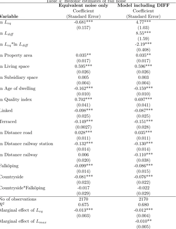
In Table 4, the results of the hedonic estimation for rail noise are presented. This includes a model with equivalent noise as the only noise variable followed by the estimated results of model (6).
All three of the noise variables in the model including multiple noise indicators are statistically significant, which suggest a good modeling choice for the noise variables. Note that both Leq and Ldiff are positive but the marginal effect need not to be positive
since we have included the interaction term and its coefficient is negative.
The marginal effects, i.e. the percentage change of an increase of 1 dB of noise evaluated at the mean noise levels, are indeed negative and also statistically significant for all noise
indicators. Interestingly, the marginal effect of Leq is very similar in the two models.
This result suggest that the incorporation of Lmax in the model, through Ldiff, do not
influence the negative effect of Leq but incorporate an additive term of disutility from the
maximum noise level.
Most of the other property characteristics are significant with the expected signs, the only non-significant variable is for subsidiary space. Accessibility and geographical vari-ables are mostly significant. Distance to road is positive which means that the positive side of living far from a road to avoid road noise and air pollution dominates the accessi-bility effect of living close to the road. The only variable with a non-expected significant sign is distance to railway which is negative, but only for the model including multiple noise indicators. Still when we model rail noise the effect of living far away from the railway can be small but it is not clear why it should be negative or differ across the models.
Table 4: Hedonic estimates of rail noise
Equivalent noise only Model including DIFF Coefficient Coefficient
Variable (Standard Error) (Standard Error)
ln Leq -0.681*** 4.77*** (0.157) (1.03) ln Ldiff 8.55*** (1.59) ln Leq*ln Ldiff -2.19*** (0.408) ln Property area 0.035** 0.035** (0.017) (0.017) ln Living space 0.595*** 0.596*** (0.026) (0.026) ln Subsidiary space 0.005 0.003 (0.004) (0.004) ln Age of dwelling -0.162*** -0.159*** (0.010) (0.010) ln Quality index 0.702*** 0.697*** (0.041) (0.041) Linked -0.098*** -0.087*** (0.025) (0.025) Terraced -0.149*** -0.151*** (0.0027) (0.028) ln Distance road 0.028*** 0.035*** (0.011) (0.011)
ln Distance railway station -0.132*** -0.130***
(0.014) (0.014) ln Distance railway 0.006 -0.110*** (0.020) (0.038) Falköping -0.099*** -0.086*** (0.014) (0.015) Countryside -0.081*** -0.076*** (0.023) (0.022) Countryside*Falköping -0.017 -0.022 (0.029) (0.029) No of observations 2170 2170 R2 0.675 0.680 Marginal effect of Leq -0.013*** -0.012*** (0.003) (0.004)
Marginal effect of Lmax -0.010**
(0.005) Notes: Dependent variable is log of annualized property price.
***, ** and * denote difference from zero at the one, five, and ten percent significance level respectively.
Yearly indicators and an intercept are also included in the model. The marginal effects are evaluated at the mean values of Leq and Lmax.
In Table 5, the results of the hedonic estimation for road noise are presented. Also for road, a model with equivalent noise as the only noise variable is presented for comparison.
The proposed model including Ldiff and the interaction between Leq and Ldiff implies a
significant equivalent noise coefficient. In addition, the marginal effects evaluated at the
mean values of Leq and Lmax show no significant effects of Lmax. We have also tested
whether the marginal effect of Lmax is significant for any of the equivalent noise levels
included in our sample and it turns out to not be. Leq is on the other hand negative and
significant at the five percent level. We therefore conclude that the inclusion of Lmax,
through Ldiff or by another structure tested in 3.1, do not add anything to a model where
the road noise effect on property prices is captured by Leq.
The explanation rate of the models is slightly lower than 0.7 which is satisfactory for this kind of micro econometric model. This is more or less in line with other comparable
hedonic model estimations of property markets.6
The implicit prices of Leq and Lmax for rail are presented in Table 6. Included as
a comparison is the implicit price of the alternative and traditional model presented in Table 4, i.e. the model with only Leqas the noise indicator. The implicit prices are defined
with a negative sign so they are expected to be positive. We can see that the implicit price of Leq are very similar across the two different models. This result is interpreted
as these two different noise costs are additive since nothing suggests that the inclusion of other noise variables besides Leq in the model decrease the implicit price of Leq. In
Section 5 the implementation of such a result in CBA will be discussed related to some concrete noise measure examples.
As a sensitivity analysis, we estimate our hedonic models on chosen parts of our full sample. These sub samples are defined with respect to regions, distance to the noise source, or noise variables, i.e. Leq and Ldiff. Especially regarding the road noise it is
interesting to analyze if another sub sample produces a significant marginal effect of
Lmax. In particular, maximum road noise may be a problem for those living really close
to a road with low traffic. Therefore it is interesting to analyze the results for properties close to the road and with high levels of Ldiff.
Table 5: Hedonic estimates of road noise
Equivalent noise only Model including DIFF Coefficient Coefficient Variable (Standard Error) (Standard Error)
ln Leq -0.003*** -0.006* (0.001) (0.003) ln Ldiff -0.005 (0.007) ln Leq*ln Ldiff 0.082 (0.136) Property area 0.031*** 0.031*** (0.008) (0.008) Living space 0.004*** 0.004*** (<0.001) (<0.001) Subsidiary space -0.226 -0.230* (0.138) (0.138) Age of dwelling -0.003*** -0.003*** (<0.001) (<0.001) Quality index 0.025*** 0.025*** (0.001) (0.001) Linked -0.120*** -0.120*** (0.019) (0.019) Terraced -0.155*** -0.155*** (0.018) (0.018) Distance road -0.097 -0.331 (0.144) (0.437)
Distance railway station -0.032*** -0.032***
(0.004) (0.004)
Distance railway -0.100 -0.085
(0.273) (0.276)
Bordering the sea/lake 0.146*** 0.146***
(0.026) (0.026) Plot hiring -0.148*** -0.148*** (0.018) (0.018) No of observations 3607 3607 R2 0.687 0.687 Marginal effect of Leq -0.003*** -0.003*** (0.001) (0.001)
Marginal effect of Lmax -0.001
(0.002) Notes: Dependent variable is log of property price.
***, ** and * denote difference from zero at the one, five, and ten percent significance level respectively.
Yearly indicators, region indicators, town area indicators, and an intercept are also included in the model.
The marginal effects are evaluated at the mean values of Leq and Lmax.
ln Leq*ln Ldiff, Property area, Subsidiary space, Distance road and Distance railway
station are divided by 1000.
Table 6: Implicit price of railway noise variables
Equivalent noise only Model including DIFF
Leq Leq Lmax 10th percentile 313 298 242 25th percentile 433 413 335 Median 578 550 446 Mean 603 574 466 75th percentile 736 701 569 90th percentile 920 876 711
First we describe the alternative models tested for both rail and road. The estimation of region-separate hedonic models does not lead to any significant results besides what is presented in the previous sections. The changes are mainly marginal and the general conclusions still hold. Furthermore, we have tested to estimate different time periods. The effect for rail is small and the noise variables are significant also in the alternative time periods. For road the result is more mixed in the sense that there are some insignificant coefficients for Leq. The other noise variables are, on the other hand, always insignificant.
Finally, we have estimated models with Lmax as the only noise variable on sub samples
including narrow intervals of Leq. This exercise results in non-significant coefficients in
all cases for rail noise and for most cases for road noise. The most interesting thing to note is that for intervals of low levels of equivalent noise, the maximum noise coefficient is insignificant also for road.
Only for rail, we have also tested to estimate the model on sub samples by excluding the lowest levels of Ldiff. This seems not to work as a good alternative to our suggested
model for rail.
Then remain the sensitivity analyses only on the road noise model. We have analyzed the maximum noise effect for properties where maximum noise level may be a substantial
problem. This is analyzed with respect to distance to road and Ldiff. We have estimated
all combinations of distance to road below 100 meters, 75 meters, or 50 meters, with Ldiff that is higher than zero or higher than 15. This means estimating the model for six
different sub samples. The results show that the marginal effect of Lmax is non-significant
in all models. Neither with these sub samples there is any evidence of a maximum noise premium for road noise besides the effect from equivalent noise. Furthermore, we have also estimated models with including longer distances to road. Here the results are not clear,
the equivalent noise is always significant while Lmax is mostly insignificant but weakly
significant in a few model specifications. Finally, we have tried to exclude distance to road from the model. This change does not lead to different results, which is not surprising since the distance to road in the estimations presented in Table 5 is not significant.
To sum up the sensitivity analysis, we have no clear evidence for not relying on the estimated models presented in the previous sub sections.
5
Discussion and implementation
As we are not aware of any previous hedonic studies where the value of the maximum traffic noise level is estimated, the starting point here is a policy discussion about the possibilities to include a maximum noise premium in cost-benefit analysis (CBA). As stated in the Introduction, there are essentially two strategies to incorporate the maxi-mum noise effect in CBA. First, you can let the WTP be a function of both the equivalent noise level and the maximum noise level. This is the strategy that we have used in this study where we model the property prices as a function of equivalent noise, the difference between the maximum noise and the equivalent noise, and an interaction term between these two variables. The other strategy at hand would be to model the property price as a function of the maximum noise level only and calculate WTP estimates based on maximum noise that can be used as a substitute to WTP estimates based on equivalent noise. The main problem with the latter approach is that it will be arbitrary which model to use in a particular situation. If some criteria would be determined, it is not clear what these criteria should be and how they should be determined. There is also a risk that such substitutable models are used in favor of an underlying objective. The problem with the latter approach means that we argue for the former approach which is also the one used in our study.
The possible implementation of our results in CBA needs to be critically discussed however. As we have estimated the hedonic price functions on the equivalent noise level and the difference between the maximum noise level and the equivalent noise level, we can calculate the implicit prices of equivalent noise and maximum noise separately. The em-pirical results presented in Table 4 suggest that, for rail noise, there are components of the individuals’ noise costs that depend on each of the noise variables. In addition, our results suggest that the marginal WTP of equivalent noise is not influenced by the inclusion of maximum noise in the model. This result contradicts the result of Baranzini and Ramirez (2005) in where the total noise cost is found to be similar regardless of the noise indicators included.
Here, we more deeply with some simple calculation examples outline how the separated maximum noise premium can be used in CBA and what the effects would be. We also base these calculations on different baseline levels of equivalent noise and maximum noise. The credibility of the results will be highest around the mean values of the noise indicators,
which is 53.3 dB for Leq and 68.4 for Lmax. The aim of this study is not to come up
with new estimates of the WTP for the equivalent noise level when the maximum noise level is unchanged and thus such WTP estimates should be taken from other sources. This happens when the traffic volume is increased; given that the noisiest train is the same one the equivalent noise level increases but the maximum noise level remains the same. Here nothing is added to CBA based on equivalent noise valuation only. The two examples, presented in Table 7, we will go through are: i, the equivalent noise level and the maximum noise level both change of the same amount in the same direction; and ii, both the equivalent noise level and the maximum noise level change in the same direction but the maximum noise level changes substantially more than the equivalent noise level. Other examples are difficult to find in the real environment regarding rail noise. This include occasions when the maximum noise level is changed but not the equivalent noise level as well as when the maximum noise level and the equivalent noise level are changed in opposite directions.
i may happen if there is some kind of noise measure taken, for example noise barriers or changed housing insulation. These measures will reduce the noise level of all noise events by approximately the same amount which reduce the equivalent noise level and the maximum noise level with the same amount. Here the WTP based on the different two model approaches are very different for some noise levels but coincides relatively well for other noise levels. Uncommon combinations and relatively extreme values of the noise variables show more variation of the estimated WTP across the models. More reliable noise levels as an equivalent noise level of 55 dB show the smallest WTP difference across the models. Noteworthy, the maximum noise level of 70 dB is closest to the sample mean and for this specific combination of noise levels, the WTP difference across the models is very small.
T able 7: WTP of differen t n o is e reducing measures i Decrease of 1 dB of b oth Leq and Lmax ii Decrease of 1 dB of Lmax and 0.4 d B of Leq Equiv alen t noise o n ly Mo del including DIFF Equiv alen t noise only Mo del including DIFF Leq 50 db: Lmax 60 db 667 0 267 0 Lmax 65 db 667 1131 267 453 Lmax 70 db 667 1745 267 698 Leq 55 db: Lmax 65 db 606 1007 242 1007 Lmax 70 db 606 671 242 671 Lmax 75 db 606 1580 242 934 Leq 60 db: Lmax 70 db 556 1938 222 1938 Lmax 75 db 556 1292 222 1292 Lmax 80 db 556 1449 222 1161 Leq 70 db: Lmax 85 db 476 2391 190 2391 Lmax 90 db 476 1793 190 1793 Lmax 95 db 476 1435 190 1435 Notes : Giv en in SEK p er prop ert y and y ear in 2009 y ear prices. T o b e included in the WTP , the implicit p ric es need to b e statistically signific a n t from zero at least at the fiv e p ercen t lev el.
ii happens if the noise level of the noisiest train change, which lead to a change of the equivalent noise level that is smaller than the change of the maximum noise level. Freight trains with traditional brakes are often the noisiest trains and if the brakes are changed to k-block brakes is one such example. Then the noise level of the most noisy train decreases and the maximum noise level can, depending on the fraction of total trains that are these freight trains, decrease much more than the equivalent noise level. Assume that the equivalent noise level decrease only with a small amount while the maximum noise level decreases substantially. Such scenario may in CBA-based policy for the equivalent noise level only, lead to a substantially downward biased welfare effect if the equivalent noise is higher than 50 dB as can be seen from Table 7. Taking the change of maximum noise into account, the welfare effect in this scenario would be substantially higher. For example, if we rely most on the estimates close to the mean values of the noise levels, the WTP when the equivalent noise level is 55 dB and the maximum noise level is 70 dB is about 3 times higher when the maximum noise level is included in the analysis. To change brakes to less noisy ones on freight train may thus be even more efficient based on the empirical results of our study.
Furthermore, it is important to discuss how the result of this study relates to the discussion of what is internalized in hedonic valuation and the health effects of traffic noise. Sleep disturbances can for example be a substantial part of the noise costs for exposed individual and sleep disturbances may be more likely when the maximum noise level is high. We do not know if sleep disturbances are internalized in the WTP based on hedonic modeling though. Unfortunately we do not observe the time schedule of the traffic and therefore neither when the trains are running. Another objection against the interpretation of the maximum noise level capturing sleep disturbances is the relevant question whether housing buyers actually know the nighttime traffic and thus the risks of sleep disturbances. This may be false for some buyers but there is of course possible that some housing buyers actually investigate a lot of property characteristics before they decide to buy a property. Still, buying a property is likely to be one of the most, if not the most, important purchases during a lifetime. Thus the conclusion is that this is a really difficult question to answer. More research is therefore needed to investigate the robustness of this finding and refinement of the empirical approach used. Still it seems promising that the model works for rail where the traffic is occasional but do not work for road where the traffic is more continuous. Other methods should be used to get insights
in what negative effects of traffic noise that are capitalized into property prices.
Regarding road noise, the non-significant effect of maximum noise along with the moderate correlation between the variables, i.e. no multicollinearity problems, lead us to the conclusion that the maximum noise has no impact on the property prices besides the equivalent noise. Then the results simply indicate that the road noise valuation is fully captured by a traditional hedonic model on the equivalent noise only. Note, however, that the structure of separate noise events on roads, as compared to railways, is difficult to capture in the type of data we used here for a hedonic analysis. There might still be occasions where the maximum road noise implies more disutility than what is captured by the equivalent noise level. To analyze areas where there are known to be low road traffic and problems of heavy vehicles or buses now and then during specific times, especially during nights, would probably be a way to capture such effects. The problem is to find such data and especially sufficient data to analyze with hedonic property pricing. Thus other methods are needed to detect these effects, e.g. stated preference (SP) approaches or difference-in-difference approaches of road traffic investments or measures. In other words, our results suggest that there is no maximum noise effect of road traffic on the WTP but, importantly, the conclusion should not be interpreted as evidence for the non-existence of such effects out there. Note also that the question of what is known to property buyers arise also regarding road noise.
6
Conclusions
In this study we have extended the traditional hedonic modeling approach of rail noise and road noise valuation to also incorporate the maximum noise levels. In other words, the estimated models are including noise indicators dependent on both equivalent noise and maximum noise.
The estimated results are different for road and rail. For road there is no evidence for a maximum noise effect on property prices besides the effect of equivalent noise. For rail, on the other hand, both the equivalent noise level and the maximum noise level are negatively influencing the property price. Based on this result, WTP of the traditional equivalent noise level and an additive WTP-part dependent on the maximum noise level are suggested to be complementary to the total rail noise costs. The marginal WTP of the maximum noise level is calculated and may be used in cost-benefit analysis. The effect of including the maximum noise level seems to be largest for a noise abatement
where the maximum noise is reduced substantially more than the equivalent noise level. One such example may be a change to noise-reducing brakes on freight trains.
Finally we want to emphasize that this is the first hedonic study where the maximum noise level is valued along with the equivalent noise and the results need to be treated with caution. More research is needed to establish the relation between the disutility of maximum noise level and equivalent noise level and the willingness to pay. Such research may be focusing on several different aspects. A few of these are; the functional form of the estimation model, the additivity between WTP for equivalent noise and maximum noise, and other approaches to estimate WTP for maximum road noise. Still we consider our study as a first insight into this problem and the suggestion that the WTP to reduce rail noise exposure does not only depend on the equivalent noise but also on the maximum noise.
References
Andersson, H., L. Jonsson, and M. Ögren: 2010, ‘Property Prices and Exposure to Mul-tiple Noise Sources: Hedonic Regression with Road and Railway Noise’. Environmental and Resource Economics 45, 73–89.
Andersson, H., J.-E. Swärdh, and M. Ögren: 2013, ‘Efterfrågan på tystnad - skattning av betalningsviljan för icke-marginella förändringar av vägtrafikbuller’. Report to swedish transport administration, VTI - Swedish National Road and Transport Research Insti-tute.
Anselin, L.: 1999, ‘Spatial Econometrics’. Mimeo, University of Texas at Dallas, USA. Baranzini, A. and J. V. Ramirez: 2005, ‘Paying for quietness: The impact of noise on
Geneva rents’. Urban Studies 42(4), 633–646.
Bristow, A. L., M. Wardman, and V. P. K. Chintakayala: 2015, ‘International meta-analysis of stated preference studies of transportation noise nuisance’. Transportation 42, 71–100.
Cameron, A. C. and P. K. Trivedi: 2009, Microeconometrics Using Stata. College Station, Texas: Stata Press.
Chen, Z. and K. E. Haynes: 2015, ‘Impact of high speed rail on housing values: an observation from the Beijing-Shanghai line’. Journal of Transport Geography 43, 91– 100.
Dekkers, J. and J. W. van der Straaten: 2009, ‘Monetary valuation of aircraft noise: A hedonic analysis around Amsterdam airport’. Ecological Economics 68(11), 2850–2858. Jonasson, H. and H. Nielsen: 1996, ‘Road traffic noise – Nordic prediction method’.
TemaNord 1996:525, Nordic Council of Ministers.
Nelson, J. P.: 2008, Hedonic Methods in Housing Markets: Pricing Environmental Ameni-ties and Segregation, Chapt. Hedonic Property Value Studies of Transportation Noise: Aircraft and Road Traffic, pp. 57–82. New York: Springer.
Ringheim, M.: 1996, ‘Railway Traffic Noise – Nordic Prediction Method’. TemaNord 1996:524, Nordic Council of Ministers, Copenhagen, Denmark. ISBN 92-9120-837-X. Rosen, S.: 1974, ‘Hedonic prices and implicit markets: Product differentiation in pure
competition’. Journal of Political Economy 82(1), 34–55.
Sheppard, S.: 1999, ‘Hedonic analysis of housing markets’. In: P. C. Cheshire and
E. S. Mills (eds.): Handbook of Regional and Urban Economics, Vol. 3 of Handbook of Regional and Urban Economics. Elsevier, Chapt. 41, pp. 1595–1635.
Small, K. A. and S. S. Steimetz: 2012, ‘Spatial Hedonics and the Willingness to Pay for Residential Amenities’. Journal of Regional Science 52(4), 635–647.
Swärdh, J.-E., H. Andersson, L. Jonsson, and M. Ögren: 2012, ‘Estimating non-marginal willingness to pay for railway noise abatements: Application of the two-step hedonic re-gression technique’. Cts working papers in transport economics, VTI - Swedish National Road and Transport Research Institute. Available at http://swopec.hhs.se/ctswps/. Swoboda, A., T. Nega, and M. Timm: 2015, ‘Hedonic analysis over time and space: The
case of house prices and traffic noise’. Journal of Regional Science. Article in Press, doi: 10.1111/jors.12187.