THEME 7
Transport including
Aeronautics
Project DELTA
C
ONCERTED COORDINATION FOR THE PROMOTION
OF EFFICIENT MULTIMODAL INTERFACES
Coordination Action Grant Agreement No: 218486
Deliverable D2.3
Knowledge Base of regions with
seasonal varying demand profiles
Version: Final
Date: December 2009
PROJECT INFORMATION
Title: Concerted coordination for the promotion of efficient
multimodal interfaces
Acronym: DELTA
Grant Agreement no: 218486
Programme: 7th Framework Programme
Funding Scheme: Coordination Action
Start date: 1st January 2009
Duration: 24 months
Web site: www.delta-project.eu
P
ROJECT
P
ARTNERS
No Name Short name Country
1
(coordinator)
Centre of Research and Technology Hellas / Hellenic
Institute of Transport CERTH/HIT Greece
2 Swedish National Road and
Transport Research Institute VTI Sweden
3 Forschungsgesellschaft Mobilitat GmbH - Austrian Mobility
Research FGM-AMOR Austria
4 Trivector Traffic AB Trivector Sweden
5 Budapest University of Technology and Economics BME Hungary
6 BDO EOS Svetovanje d.o.o. BDO EOS Slovenia
7 MIZAR Automazione S.p.A. MIZAR Italy
8 Universita degliStudi di Salerno Usalerno Italy
9 Anatoliki S.A. Development Company REACM Greece
10 Segura Durán Assessors S.A. SD Assessors Spain
11 Ente Autonomo Volturno EAV Italy
12 Municipality of Solcava Solcava Slovenia
DOCUMENT PROFILE
Document status: Final
Deliverable code: D2.3
Deliverable title: Knowledge Base of regions with seasonal varying
demand profiles
Work Package: WP2
Preparation date: December 2009
Submission date: December 2009
Total pages: 35
Dissemination level: Public
Author: Kerstin Robertson, VTI
Contributors: Rune Karlsson, VTI
Annie Kortsari, CERTH Yannis Tyrinopoulos, CERTH
Abstract: This document describes the work carried out for
developing the Knowledge Base in WP 2, Task 2.5 Development of a Knowledge Base of cities with seasonal demand. Data was delivered from Task 2.3 (IR2.1 Data collection report from participating regions) and Task 2.4 (IR2.2 Data collection report from additional regions). The knowledge database is delivered in an MS Access (2003 or 2007) file, which is provided as an Annex to this report and can be downloaded from the website of the project (www.delta-project.eu). The development of the Knowledge Base was carried out by VTI.
EXECUTIVE SUMMARY
This document describes the work carried out for developing the Knowledge Base in WP 2, Task 2.5 Development of a Knowledge Base of cities with seasonal demand. Data was delivered from Task 2.3 (IR2.1 Data collection report from participating regions) and Task 2.4 (IR2.2 Data collection report from additional regions). The knowledge database is delivered in an MS Access (2003 or 2007) file, which is provided as an Annex to this report and
can be downloaded from the website of the project (www.delta-project.eu).
The database has been structured into several tables. Also, several functions for analyzing data have been included.
In this document the basic data tables are described. A section which describes the output from computations is also included.
CONTENTS
1. Introduction__________________________________________________________ 7
1.1. Short introduction to the Delta project ____________________________ 7
1.2. Scope and role of the Knowledge Base___________________________ 7
1.3. Content and structure of the report_______________________________ 8
2. Requirements and installation procedures for the DELTA Knowledge Base
10
2.1. System requirements____________________________________________ 10
2.2. Database installation ___________________________________________ 10
2.3. Potential problems to be encountered in the course of the use of the
Knowledge Base ______________________________________________________ 10
3. Description of the DELTA Knowledge Base ____________________________ 12
3.1. The regions_____________________________________________________ 12
3.2. Design _________________________________________________________ 13
3.3. Structures of the basic data tables_______________________________ 13
3.3.1. General data ______________________________________________ 14
3.3.2. Quantitative data __________________________________________ 15
3.3.3. Qualitative data ___________________________________________ 16
3.3.4. Relations between tables ___________________________________ 21
3.4. Running the Knowledge Base ___________________________________ 21
3.5. Operations and results of the database__________________________ 23
3.6. Looking deeper into the Knowledge Base________________________ 33
LIST OF TABLES
Table 1: Regions participating in the Delta project_________________________ 12 Table 2: Additional regions _______________________________________________ 12 Table 3: The structure of the database table RegionNames ________________ 14 Table 4: The structure of the database table DataSources _________________ 14 Table 5: The structure of the database table Interviewees _________________ 14 Table 6: The structure of the database table Quant_Questions _____________ 15 Table 7: The structure of the database table Quant_Values ________________ 16 Table 8: The structure of the database table Qual_Questions ______________ 17 Table 9: The structure of the database table Qual_Numeric________________ 18
Table 10: The structure of the database table Qual_Descriptions ___________ 19 Table 11: The structure of the database table Qual_Comments ____________ 19 Table 12: The structure of the database table Qual_Sources _______________ 20 Table 13: The structure of the database table Qual_Interviewees___________ 20 Table 14: The subforms and subqueries used in the computations __________ 34
L
IST OF
F
IGURES
Figure 1: Example of records in the table Quant_Questions ________________ 16 Figure 2: Some records in table Qual_Questions ___________________________ 18 Figure 3: Relations between quantitative data tables______________________ 21 Figure 4: Relations between qualitative data tables _______________________ 21 Figure 5: The main form in the Knowledge Base. ___________________________ 22 Figure 6: Outputs from operation No 1 ____________________________________ 24 Figure 7: Outputs from operation No 2 ____________________________________ 25 Figure 8: Outputs from operation No 3 ____________________________________ 26 Figure 9: Outputs from operation No 4 ____________________________________ 27 Figure 10: Outputs from operation No 5 ___________________________________ 28 Figure 11: Outputs from operation No 6 ___________________________________ 29 Figure 12: Outputs from operation No 7 ___________________________________ 29 Figure 13: Outputs from operation No 8 ___________________________________ 30 Figure 14: Outputs from operation No 9 ___________________________________ 30 Figure 15: Outputs from operation No 10 __________________________________ 31 Figure 16: Selecting a specific variable ___________________________________ 32 Figure 17: Outputs from operation No 12 __________________________________ 32 Figure 18: Outputs from operation No 15 __________________________________ 33 Figure 19: Outputs from operation No 16 __________________________________ 33
ANNEX
Annex 1: Data and results of the Knowledge Base of regions with seasonal transport demand profiles
1. INTRODUCTION
1.1. Short introduction to the Delta project
DELTA is a research project, which addresses regions that suffer from strong and seasonal variations of transport demand causing congestion, environmental pollution, energy loss, increased travel times and other negative effects. The project will define and validate intelligent mobility tools and practices guidelines, as well as policy guidelines addressing the optimum management of seasonal demand for transport areas with proven relevant problems.
The launching of the DELTA project represents a transnational and trans-sectorial activity of various European regions, which stresses two of the most important issues of the sustainable mobility development by involving both the tourism and transport sector. The project will provide viable solutions for accessibility, spatial development and transport by the promotion of sustainable public transport.
The main outcome of the DELTA project is the Decision Support Instrument (DSI) composed of a set of roadmaps to promote intelligent and sustainable mobility in areas with varying demand of passenger transport. This innovative tool embodies critical factors affecting variations of transport demand as well as strategies, policies and measures adaptive to the local conditions aiming to smooth out the varying transport demand in the target regions.
Apart from the DSI, the project outcomes will be enhanced by various intermediate products, among them a detailed database or Knowledge Base that will include all the collected information for cities across Europe and their characteristics concerning their transport systems, mobility management and intelligent/innovative mobility schemes. This outcome is an important contribution of the DELTA project since it includes the factors and variables that affect the variability of transport demand in the concerned areas.
1.2. Scope and role of the Knowledge Base
The Knowledge Base will be one of the key outcomes of the project, as it will contain all the necessary information to be used by the work packages that follow, which regard the classification of regions, the framework of mobility schemes (WP 3) and the definition of the DSI (WP 4). Indicative data to be archived are the factors and variables that affect the variability of transport demand, the characteristics of the cities, local policies and measures of mobility management, etc.
In WP 3 an analysis of the data archived in the Knowledge Base will be conducted that will lead to the classification of the cities in a small number of broad categories. In particular, a categorical analysis will be applied and the main criteria to be used will be several measures of effectiveness, such as percentage of reduction in seasonal demand, GDP, city size, network size on-
and off-peak passenger/kilometres, frequency of services, mean cost of transit etc. The cities inventory and their classification based on their profile will allow the development of a Framework of all mobility strategies and related measures applied per category (class) to handle seasonal peaks.
These previous tasks will contribute to the development of a Benchmarks Handbook, constituting the consolidation and sound presentation of the identified benchmarks for cities with varying and seasonal peak problems. The benchmarks will be consolidated per city class according to the cities classification they will be mapped against the Framework of mobility schemes.
The two work packages (WP 2 and 3) will contribute to the development of the DELTA Decision Support Instrument (DSI) composed of Roadmaps of associated integrated, intelligent mobility strategies and measures. Each roadmap will actually be a sequence of mobility strategies and measures for a successful handling of seasonal peaks and the achievement of integrated, intelligent and sustainable mobility. The roadmaps will be developed using the Cities Classification (profiles), the Framework of mobility schemes, based on the Knowledge Base, and the Benchmarks Handbook.
Finally, it should be noted that the present report is the actual deliverable of task 2.3 while the Knowledge Base which has been created in an Access form, is considered an Annex to this report. This Annex is available to all interested parties in the official website of the DELTA project (www.delta-project.eu). The actual link for the database is the following:
http://www.delta-project.eu/Outcomes/tabid/59/Default.aspx
1.3. Content and structure of the report
In this report, the result of the work done during Task 2.5 (Development of a Knowledge Base of cities with seasonal demand) is presented. The Knowledge Base has been realized as an Access database essentially containing:
• Basic data tables, containing all data collected in Tasks 2.3 and 2.4. • Tools for quickly analyzing and comparing the data. For instance,
comparisons between high and low seasons quantities can be done very conveniently.
Much effort has been put into structuring the basic tables in a logical and efficient way. The structure of these tables is defined in detail in the report. Also, a detailed description of the analysis tools is presented, including how to use them and what their outputs actually mean.
In chapter 2, the system requirements and installation procedures for the Knowledge Base are described, together with some potential problems that might be encountered by the user in the course of the use of the Knowledge Base.
Chapter 3 contains an account of the contents of the database as well as its tools for analysing data. More specifically, the regions from which data have been collected are listed, while the design policy of the basic data tables in the Knowledge Base is also briefly presented. A very detailed description of these tables is given, together with instructions on how to run the tools in the Knowledge Base. Following, a very detailed description over the operations and their outputs is included. Finally, several pieces of information are given for those users interested in the implementation details and the program code.
As already mentioned above, the present deliverable is accompanied by an Annex which comprises the actual Knowledge Base in Access Form. All the data collected and the computations described throughout this document can be found in this database.
2. REQUIREMENTS AND INSTALLATION
PROCEDURES FOR THE
DELTA
K
NOWLEDGE
B
ASE
2.1. System requirements
The Delta Knowledge Base can be run on any Windows computer having either Microsoft Access 2003 or 2007 installed. The memory requirements are very limited.
2.2. Database installation
The Knowledge Base is delivered in the file
Delta_DB_2009-12-14_FINAL_revised.mdb. It can be run with either MS Access 2003 or MS Access
2007. No special installation procedure is needed. The Knowledge Base is started by double-clicking the file or by opening it from within Access.
2.3. Potential problems to be encountered in the
course of the use of the Knowledge Base
When starting the Knowledge Base a security warning message might be shown.
Access 2003: Press button “Open” to continue.
Access 2007: By default the warning message “Security Warning: Some
content in the database has been deactivated.” is displayed immediately
below the tools menu1. Press the button “Options ...” and select “Activate
content”.
1 This warning message is not very conspicuous and is easily neglected by the user.
The annoying consequence of this might be that the program halts waiting for an input to the message, while to the user the program appears to have stopped working.
It is possible to prevent the warning message to appear:
Open Access 2007 and create a new empty database. Press the "Office button" and then the "Access options ..." button below. Select "Security center" in the list and then press the button to the right. In the new form that opens you select "Macro settings" and "Enable all macros ..".Then exit Access. After this has been done you should be able to open the .mdb file without problems.
Important note only for Access 2003 Service Pack 3:
MS Access 2003 SP3 suffers from a Microsoft recognized bug which affects the Delta Knowledge Base. It makes contents in list boxes invisible. There exists a hotfix for this bug that can be downloaded from the Microsoft web site:
http://download.microsoft.com/download/6/4/0/640eb828‐5556‐4588‐8e1a‐
66fe8e0e3ad9/office2003‐kb945674‐glb.exe
1. Run the above Microsoft exe-file. It downloads the file MSACCESS.msp . 2. Double-click on MSACCESS.msp for installing the hotfix.
After this has been done the Knowledge Base should run properly.
Important
The tables, queries and forms in the database whose name has a prefix (tbl, qry, frm, subfrm) should not be changed. These are “system” objects used by the routines performing the computations in the database.
3. DESCRIPTION OF THE DELTA KNOWLEDGE
B
ASE
3.1. The regions
Definition and acquisition of data to be included in the Knowledge Base was conducted during Task 2.2 Description of structured data collection mechanism (Deliverable D2.2 Data collection mechanism (DCM)). The definition of data was based on the requirements in Work package (WP) 3 Classification of cities and mobility schemes and 4 Definition of Decision Support Instrument (DSI). Data collection from participating regions was carried out in Task 2.3 (Internal Report IR2.1) and from additional regions in Task 2.4 (Internal Report IR2.2).
Data from the following regions is included in the Knowledge Base (Table 1 and Table 2):
Table 1: Regions participating in the Delta project
PARTICIPATING REGIONS COLLECTED BY DELTAPARTNERSpain (E): Balearic islands SD Assessors
France (F): Arcachon Bay,
Lourdes CETE SO
Sweden (S): Öland VTI
Greece (GR): Chalkidiki region REACM and CERTH/HIT
Italy (I): Ischia island USalerno and EAV
Slovenia (SLO): Logarska
dolina BDO EOS and Solcava
Hungary (H): Lake Balaton BME
Table 2: Additional regions
ADDITIONAL REGIONS COLLECTED BY DELTAPARTNER
Slovenia (SLO): Bled, Kranjska
Gora, Zrece, Izola, Kamnik BDO EOS and Solcava
Hungary (H): Danube-bend,
Lake Tisza BME
Greece (GR): Thassos, Florina REACM and CERTH/HIT
Italy (I): Amalfi coast, Cilento coast
USalerno and EAV
Austria (AU): South-West Styria FGM-AMOR
France (F): Bascue coast CETE SO
3.2. Design
During the data collection phase data was compiled in two formats, Microsoft Excel format for the quantitative data and Microsoft Word format for the qualitative data. In order to make all data easily accessible in one database (Knowledge Base) it was decided to develop an Access data base that provides maximum flexibility for further analyses of the collected data, including combined analyses of quantitative and qualitative data. The database should also contain a set of tools for analyzing the data.
When designing the basic data tables some principles were aimed at:
• The database should contain no redundancies. One piece of information should exist only at one place in the database.
• The data collection questionnaires already had a certain structure. This structure should be reflected in the database tables.
• The structure should be as simple as possible.
• It should be easy to compute results from the tables in the database. It was natural to separate qualitative data from quantitative data and put these into different tables. Qualitative data is a mixture of numerical and non-numerical values, while quantitative data consists only of non-numerical values. Moreover, in the questionnaire, qualitative data, in contrast to quantitative data, is usually organised in clusters.
All quantitative data has been stored in one single data table. In contrast, the qualitative data has been split into five different tables. The structure of the questionnaires is described in two other tables, one for the quantitative and one for the qualitative case. Finally, in two additional tables, information concerning data sources and interviewees is stored.
A more detailed description over the basic data tables in the Knowledge Base is found in section 3.3.
3.3. Structures of the basic data tables
In this section the basic data tables in the database are described. All computations that are done in the Knowledge Base are based on the contents of these tables.
3.3.1. General data
Region Names
For each region a three letter code has been defined in order to facilitate the computations. The database table “RegionNames” specifies the code and the full name for each region.
Table 3: The structure of the database table RegionNames
Field
name Description
CODE Three letter code for the region
NAME Name of the region in clear text
COUNTRY Country in which the region is located
Data Sources
For the collection of qualitative data various (written) sources have been used. The database table “DataSources” contains a list over all these sources. REGION_ID combined with DATASOURCE_NO provides a unique identifier for a data source.
Table 4: The structure of the database table DataSources
Field name Description
REGION_ID Three letter code for the region that the data source
describes. (Corresponds to CODE in table RegionNames.) DATASOURCE_NO Identifier for the data source (unique for a specific region)
SOURCE Description of the data source
Interviewees
Qualitative data often consists of subjective judgements made by carefully chosen persons in key positions (interviewees). The database table “Interviewees” contains a list of all the participating interviewees as well as several information regarding them, such as the organizations they belong to and the positions they hold in them.
REGION_ID combined with INTERVIEWEE_NO provides a unique identifier for an interviewee.
Table 5: The structure of the database table Interviewees
REGION_ID Three letter code for the region that the interviewee has provided information. (Corresponds to CODE in table RegionNames.)
INTERVIEWEE_NO Identifier for the interviewee (unique for a specific region)
NAME_ORG Name of the organisation which the interviewee represents
TYPE_ORG Type of the organisation
ROLE_ORG Role of the organisation
NAME_INT Name of the interviewee
POSITION_INT Position of the interviewee
ADDRESS Address to the interviewee
TELEPHONE Telephone number to the interviewee
FAX Fax to the interviewee
EMAIL Email to the interviewee
3.3.2. Quantitative data
Quant Questions
The database table “Quant_Questions” reflects the structure of the quantitative questionnaire (i.e. the Excel sheet that was used as a template when collecting the data). Each record in this table corresponds to one specific item (question) in the questionnaire. A unique identifier has been defined for each such item.
Table 6: The structure of the database table Quant_Questions
Field name Description
ID A unique identifier for the question. It is a text string of varying
length. The ID has been constructed so that the user in most cases should be able to guess which question it refers to.
NUMBER The questions in the questionnaire are ordered in a specific
sequence. NUMBER specifies the order number within that sequence. Its main purpose is to make it possible to display results in the same order as in the questionnaire. Also, it is sometimes more convenient to use an integer than a text string when making selections of records.
TOPIC The general topic to which the question belongs. Usually the
same text as in the questionnaire.
SUBTOPIC The subtopic to which the question belongs. Usually the same
text as in the questionnaire.
as in the questionnaire.
SUBVARIABLE The subvariable to which the question refers. Usually the same text as in the questionnaire.
UNIT The unit for the data
The purpose of the fields TOPIC, SUBTOPIC, VARIABLE and SUBVARIABLE is to make it clearer to the user to which questions displayed results refer to. There exists a one-to-one correspondence between the questions in the questionnaire, the identifier (ID) and the quadruple (TOPIC, SUBTOPIC, VARIABLE, SUBVARIABLE).
In Figure 1, the first nine records in table “Quant_Questions” are shown.
ID NUMBER TOPIC SUBTOPIC VARIABLE SUBVARIABLE UNIT GEO_SIZE 1 Region chaGeographica1. Size of the km2 GEO_MUNICIPS_NUM 2 Region chaGeographica2. Number o Municipalities Number GEO_PROVINCES_NUM 3 Region chaGeographica2. Number o Provinces Number GEO_NUM_TOWNS 4 Region chaGeographica2. Number o Town (>200 inhNumber GEO_VILLAGES_NUM 5 Region chaGeographica2. Number o Village Number GEO_USES_AGRICULTURAL 6 Region chaGeographica3. Land Use Agricultural % GEO_USES_INDUSTRIAL 7 Region chaGeographica3. Land Use Industrial % GEO_USES_RESDIENTIAL 8 Region chaGeographica3. Land Use Residential % GEO_USES_TOURISM 9 Region chaGeographica3. Land Use Tourism facilitie%
Figure 1: Example of records in the table Quant_Questions
Quant Values
All quantitative data collected in WP 2.3 and 2.4 have been gathered in one single table: “Quant_Values”. For each question and region a unique numeric value is stored.
Table 7: The structure of the database table Quant_Values
Field name Description
QUESTION_ID The unique identifier for the question. (Corresponds to ID in table Quant_Questions)
REGION_ID The three letter code for the region (Corresponds to CODE in
table RegionNames)
VALUE The numerical value. (The Access data type is Double,
although both integers and floating numbers are stored here.)
ID A record ID. Not used.
3.3.3. Qualitative data
The database table “Qual_Questions” reflects the structure of the qualitative questionnaire. It is the analogue to “Quant_Questions” for quantitative data.
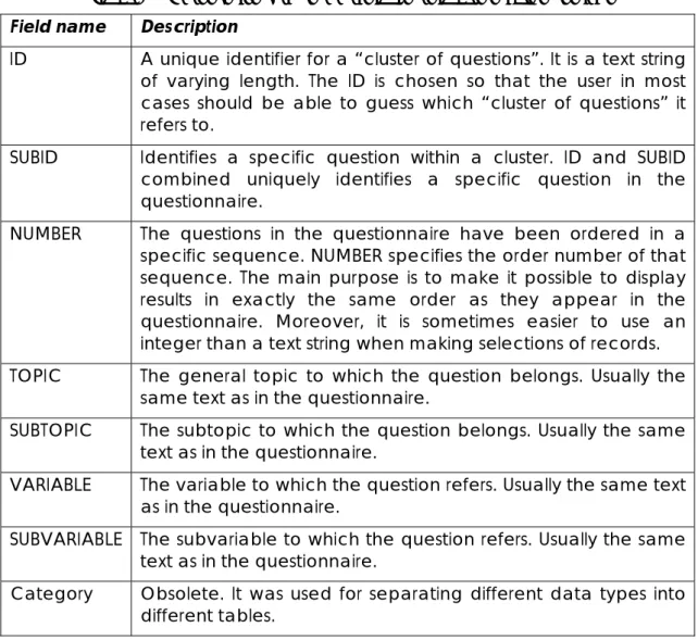
Table 8: The structure of the database table Qual_Questions
Field name Description
ID A unique identifier for a “cluster of questions”. It is a text string
of varying length. The ID is chosen so that the user in most cases should be able to guess which “cluster of questions” it refers to.
SUBID Identifies a specific question within a cluster. ID and SUBID
combined uniquely identifies a specific question in the questionnaire.
NUMBER The questions in the questionnaire have been ordered in a
specific sequence. NUMBER specifies the order number of that sequence. The main purpose is to make it possible to display results in exactly the same order as they appear in the questionnaire. Moreover, it is sometimes easier to use an integer than a text string when making selections of records.
TOPIC The general topic to which the question belongs. Usually the
same text as in the questionnaire.
SUBTOPIC The subtopic to which the question belongs. Usually the same
text as in the questionnaire.
VARIABLE The variable to which the question refers. Usually the same text
as in the questionnaire.
SUBVARIABLE The subvariable to which the question refers. Usually the same text as in the questionnaire.
Category Obsolete. It was used for separating different data types into
different tables.
There are some important differences in the structures of tables “Quant_Questions” and “Qual_Questions”. All quantitative data are numeric, while qualitative data is a mixture of text and numeric types. Moreover, qualitative data are often structured in “clusters” of which some data may be texts while others are numeric. (A cluster may typically consist of a rate, comments, interviewees and data sources). Therefore, it was found appropriate to introduce two identifiers: one (ID) identifying the cluster and another one (SUBID) identifying the specific question within the cluster.
In Figure 2, three different clusters are displayed. The first (GEO_TOPO) corresponds to the variable “Topography/Geography”. It consists of five specific questions, two of these being of numeric type, while the others are text. They are distinguished by their different SUBID.
ID SUBID NUMBER TOPIC SUBTOPIC VARIABLE SUBVARIABLE Category GEO_TOPO DESCR 1 Region chaGeographica 1. Topography/GeDescription PM GEO_TOPO HIGHEST 2 Region chaGeographica 1. Topography/GeHighest point (meNUM GEO_TOPO LOWEST 3 Region chaGeographica 1. Topography/GeLowest point (me NUM GEO_TOPO INT 4 Region chaGeographica 1. Topography/GeInterviewee No: INT GEO_TOPO SRC 5 Region chaGeographica 1. Topography/GeData source No: SRC GEO_CLIMATE_ZONE DESCR 6 Region chaGeographica 2. Climate z Description PM GEO_CLIMATE_ZONE COM 7 Region chaGeographica 2. Climate z Comments: COM GEO_CLIMATE_ZONE INT 8 Region chaGeographica 2. Climate z Interviewee No: INT GEO_CLIMATE_ZONE SRC 9 Region chaGeographica 2. Climate z Data source No: SRC GEO_CLIMATE_LIMITS DESCR 10 Region chaGeographica 3. Describe Description PM GEO_CLIMATE_LIMITS INT 11 Region chaGeographica 3. Describe Interviewee No: INT GEO_CLIMATE_LIMITS SRC 12 Region chaGeographica 3. Describe Data source No: SRC
Figure 2: Some records in table Qual_Questions
The different data types for different SUBID within a cluster make it suitable to store data in separate tables, defined by the field “Category”. There are five different “natural” categories:
• PM: texts (sometimes very long) • NUM: numerical data
• COM: comments
• INT: comma-separated list of interviewee numbers • SRC: comma-separated list of data source numbers
(The COM, INT, SRC categories could, of course, have been included in the PM category. However, since these quantities appear very regularly in most clusters it was natural to assign separate classes for them.)
For each of these categories, data have been gathered into a separate table. Each of these is described in the sequel.
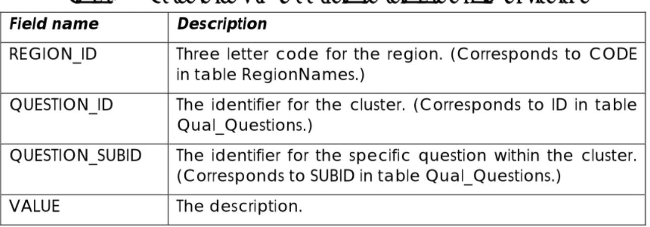
Qual Numeric
Qualitative data may sometimes be numeric. This is typically the case for subjective ratings made by the interviewees of various features (rates are being integers between 1 and 5). For instance, in Figure 2 the cluster GEO_TOPO contains two numeric questions having SUBID = HIGHEST and SUBID=LOWEST respectively. The cluster GEO_CLIMATE_ZONE, however, contains no numerical questions. The database table “Qual_Numeric” contains all numerical qualitative data.
Table 9: The structure of the database table Qual_Numeric
Field name Description
REGION_ID Three letter code for the region. (Corresponds to CODE
in table RegionNames.)
Qual_Questions.)
QUESTION_SUBID The identifier for the specific question within the cluster.
(Corresponds to SUBID in table Qual_Questions)
VALUE The numerical value
Qual Descriptions
Qualitative data are often long textual descriptions. These have been collected in the database table “Qual_Descriptions”. (Note that comments have not been included here and are instead compiled in a separate table.)
Table 10: The structure of the database table Qual_Descriptions
Field name Description
REGION_ID Three letter code for the region. (Corresponds to CODE
in table RegionNames.)
QUESTION_ID The identifier for the cluster. (Corresponds to ID in table
Qual_Questions.)
QUESTION_SUBID The identifier for the specific question within the cluster.
(Corresponds to SUBID in table Qual_Questions.)
VALUE The description.
Note that VALUE has the MS Access data type “PM”, since the descriptions sometimes exceed the maximum allowed lengths for the data type “Text” (255 characters).
Qual Comments
All comments have been collected in one database table, “Qual_Comments”. Most of the clusters have a comment item.
Table 11: The structure of the database table Qual_Comments
Field name Description
REGION_ID Three letter code for the region. (Corresponds to CODE
in table RegionNames.)
QUESTION_ID The identifier for the cluster. (Corresponds to ID in table
Qual_Questions.)
QUESTION_SUBID The identifier for the specific question within the cluster.
(Corresponds to SUBID in table Qual_Questions.)
VALUE has the data type “PM”.
Qual Sources
The sources are specified by a comma separated sequence of integers, representing the numbers of the data sources. This is suitably stored as a text string.
Table 12: The structure of the database table Qual_Sources
Field name Description
REGION_ID Three letter code for the region. (Corresponds to CODE
in table RegionNames.)
QUESTION_ID The identifier for the cluster. (Corresponds to ID in table
Qual_Questions.)
QUESTION_SUBID The identifier for the specific question within the cluster.
(Corresponds to SUBID in table Qual_Questions.)
VALUE A text string consisting of a sequence of ID numbers of
the data sources. (See Table 4.)
Note that the way that has been chosen in order to represent the data sources here makes it difficult to join the tables “Qual_Sources” and “DataSources”. It was considered, however, that such a join was not of much interest to the present task.
Qual Interviewees
The interviewees are specified by a comma separated sequence of integers. This is suitably stored as a text string.
Table 13: The structure of the database table Qual_Interviewees
Field name Description
REGION_ID Three letter code for the region. (Corresponds to CODE
in table RegionNames.)
QUESTION_ID The identifier for the cluster. (Corresponds to ID in table
Qual_Questions.)
QUESTION_SUBID The identifier for the specific question within the cluster.
(Corresponds to SUBID in table Qual_Questions.)
VALUE A string consisting of a sequence of ID numbers of the
3.3.4. Relations between tables
No explicit relations between the database tables have been defined à priori. Instead, the relations must be defined for each query that is constructed.
In Figure 3, relations between quantitative tables, necessary to use when a query is defined, are shown. The identifier field (ID) in the database table “Quant_Questions” is connected to the field Question_ID in the database table “Quant_Values”.
In Figure 4, relations between qualitative tables are shown. Besides the cluster identifier (ID) there was also need to connect the SUBID field.
Figure 3: Relations between quantitative data tables
Figure 4: Relations between qualitative data tables
3.4. Running the Knowledge Base
In this section the actual way to run the Knowledge Base is described. A more detailed description is presented in section 3.5.
The Knowledge Base is started by double-clicking the file or by opening it from Access.
A welcome window opens automatically. Click on the “Open” button to open the Delta main form.
In the main form one can choose between several operations. After selecting an operation in the “Select operation” list box, the “RUN” button is clicked and the result is shown in the grid below, see Figure 5. For some of the operations an additional selection of a specific topic and variable in the list boxes has first to be done before clicking the “RUN” button.
Clicking on the button “Close form”, closes the main form and Access main screen becomes visible.
NOTE 1: Empty cells in the Results grid signify either missing values or results where division by zero has occurred. The latter may for instance occur when computing relative increases from low to high seasons for variables having zero values.
NOTE 2: The contents in the Results grid can be cut and pasted into e.g. Excel. The grid can be sorted with respect to any column (Access 2007: use the arrow in the header, Access 2003: right-click the column). Also the width of each column can be changed as well as the height of each row. The latter can be useful when the grid contains long texts.
3.5. Operations and results of the database
In this section, all the predefined operations (analysis tools) listed in the “Select operation” list box in the main form are described in more detail as well as several results from these operations.
Note that “increase” is here defined as (High-Low)/Low, where “High” denotes the high season value for a variable and “Low” the corresponding low season value. The increases are expressed in terms of percentages.
Operations 1-5 and 11-15 are based on quantitative data only. The remaining operations are based on qualitative data.
Operation 1. Determine for various modes of transport the percentage
increase in traffic volumes from low to high seasons.
The increase in traffic volume from low to high season is an important characteristic for the seasonal variation. Traffic volume can be defined in different ways. In this operation the following quantities for the different modes have been used:
Cars: Number of vehicles per day (question C.2.17 in the questionnaire)
Railway: Number of passengers per day – Within region (C.3.19)
Waterways: Number of passengers per day – Within region (C.4.9 )
Airways: Number of passengers per day – Within region (C.5.2)
When running this operation from the main form the result becomes as shown in Figure 6.
In many cases a transport mode is not relevant for a region. For instance, there are no railways, waterways or airfields in the Malung-Sälen region. Consequently, the corresponding cells in the grid in Figure 6 are left empty. In many cases data concerning traffic volume was not available. The missing values are also represented by empty cells. Unfortunately, there is no way to distinguish these two categories in the figure.
NAME COUNTRY VOL_CARS RAIL_PASS WATER_PASS AIR_PASS Amalfi Coast Italy Archacon Bay France 15.80% Balearic Island Spain 44.40% 33.30% 50.00% 22.30% Bascue coast France Bled Slovenia Chalkidiki Greece 208.50% Cilento Coast Italy Dunakanyar Hungary 12.80% Florina Greece Ischia Island Italy Izola Slovenia Kamnik Slovenia Kranjska Gora Slovenia Lake Balaton Hungary 144.00% 108.70% 788.90% Logarska dolina Slovenia 58.30% Lourdes France 244.40% Lysekil Sweden 100.00% 250.00% Malung‐Sälen Sweden 152.00% SW Styria Austria Thassos Greece Tisza Hungary 190.70% 88.80% Zrece Slovenia Öland Sweden 66.70%
Figure 6: Outputs from operation No 1
Operation 2. Determine the bus load factor (percentages) during high season.
The bus load factor is the average passenger occupancy of the busses. (Number of passengers divided by the capacity.) This indicator can give a picture over the potential for expanding public transports in the region. In Figure 7, bus load factors for high season are shown.
Region name Country name Bus load factor [%] Lourdes France 100.00% Balearic Island Spain 95.00% Chalkidiki Greece 90.00% Thassos Greece 70.00% Izola Slovenia 65.00% Ischia Island Italy 60.00% Kranjska Gora Slovenia 50.00% Zrece Slovenia 45.00% Lake Balaton Hungary 41.00% Logarska dolina Slovenia 40.00% Bled Slovenia 35.00% Kamnik Slovenia 35.00% Florina Greece 30.00% Archacon Bay France Bascue coast France Tisza Hungary Dunakanyar Hungary Lysekil Sweden SW Styria Austria Amalfi Coast Italy Malung‐Sälen Sweden Öland Sweden Cilento Coast Italy
Figure 7: Outputs from operation No 2
Operation 3. Determine the percentage increase in road accidents from low
to high season.
The output from operation no 3 is shown in Figure 8. Road accidents here mean: number of road accidents with cars involved (C.1.1).
For road accidents in general, the numbers are rather low for some regions. Hence, the relative increase can be rather unreliable, in some cases even negative.
Region name Country name Increase in road accidents Archacon Bay France 900.00% Balearic Island Spain 367.10% Öland Sweden 241.40% Malung‐Sälen Sweden 233.30% Lake Balaton Hungary 105.90% Chalkidiki Greece 78.60% Thassos Greece 22.40% Kamnik Slovenia 18.00% Florina Greece 12.50% Bascue coast France ‐2.70% Lourdes France ‐10.70% Lysekil Sweden ‐40.00% Bled Slovenia Cilento Coast Italy Dunakanyar Hungary Ischia Island Italy Amalfi Coast Italy Kranjska Gora Slovenia Logarska dolina Slovenia SW Styria Austria Tisza Hungary Zrece Slovenia Izola Slovenia
Figure 8: Outputs from operation No 3
Operation 4. Determine the percentage increase in the number of visitors from
low to high season.
Region name Country name Increase in number of visitors SW Styria Austria 3992.80% Lysekil Sweden 2450.00% Öland Sweden 1550.00% Malung‐Sälen Sweden 1200.00% Cilento Coast Italy 1149.80% Lake Balaton Hungary 900.00% Logarska dolina Slovenia 802.20% Lourdes France 733.30% Balearic Island Spain 500.00% Izola Slovenia 239.50% Bascue coast France 233.30% Zrece Slovenia 182.00% Kamnik Slovenia 180.00% Bled Slovenia 150.80% Kranjska Gora Slovenia 82.90% Ischia Island Italy 28.60% Amalfi Coast Italy 20.00% Florina Greece Dunakanyar Hungary Chalkidiki Greece Thassos Greece Tisza Hungary Archacon Bay France
Figure 9: Outputs from operation No 4
Operation 5. Determine the percentage increase in passenger-km by cars
from low to high season.
Passenger-km by cars here includes both drivers and passengers. Evidently, data for this indicator has been difficult to collect and values are missing for a majority of regions.
Region name Country name Increase in pass‐km by cars Öland Sweden 558.50% Lysekil Sweden 557.40% Tisza Hungary 386.10% Lake Balaton Hungary 199.10% Malung‐Sälen Sweden 10.80% Dunakanyar Hungary 6.20% Balearic Island Spain ‐30.80% Kranjska Gora Slovenia Archacon Bay France Bascue coast France Bled Slovenia Chalkidiki Greece Cilento Coast Italy Florina Greece Ischia Island Italy Amalfi Coast Italy Kamnik Slovenia Logarska dolina Slovenia Lourdes France SW Styria Austria Thassos Greece Zrece Slovenia Izola Slovenia
Figure 10: Outputs from operation No 5
Operation 6. Determine the main causes that contribute to traffic congestion
and other major disturbances.
In the qualitative questionnaire the interviewees were asked to give their opinion, in terms of grades or rates, on the degree of influence on congestion in their respective region, for certain possible causes. The rate=1 should signify very little importance while the rate=5 signifies a very important cause. This information is stored in the basic data table “Qual_Numeric”, see Table 9. In Figure 11, the average rate taken over all regions have been computed for each potential cause for congestion. The results have been sorted in decreasing order. It was concluded that “Unnecessary use of cars for short trips” is in general rated as an important cause for congestion by the interviewees.
Congestion causes Rates: 1=least important, 5=most important Unnecessary use of cars for short trips 3.8 Lack of alternatives modes of transport 3.55 Lack of cooperation between modes of transport 3.45 Lack of legal parking spots 3.4 Insufficient transport network 3.211 Lack of free parking spots 3.211 Low frequency of public transport services 3.158 Lack of cycle lanes 3.158 Bad transport network 3.105 Public transport of low quality 2.9 Lack of systems for mobility support 2.647 Lack of traffic management centres 2.6 Lack of information regarding alternatives modes of transp 2.5 High cost of available parking spots urging citizens to illega 2.25 High fares in alternative modes of transport 2.2 Lack of on line booking systems for local tourism services h 2.1
Figure 11: Outputs from operation No 6
Operation 7. Determine the most important effects of seasonal traffic.
The results in Figure 12 have been generated by running query no 7. Various effects of seasonal traffic have been rated by the interviewees from each region. Averages of the rates over all regions are shown. It is clear that congestion and increased travel times are judged (on average) to be the most important consequences of seasonal traffic.
Effects of seasonal traffic Rates: 1=least important, 5=most important Congestion in the transport routes 4.524 Increased travel times 4.143 Increase of the number of accidents 3.571 Energy loss 3.55 High CO2 emissions 3.286 Damage to the natural environment 3.238 Low quality of offered services 3.095 Severe noise pollution 3.048 Damage of the transport infrastructure 2.762 Harms to the historical sites 2.45
Figure 12: Outputs from operation No 7
Operation 8. List systems used for mobility support.
In Figure 13 systems used for providing travelers with information that will make it easier to find public transport departures and connections are listed.
Region name Country name Systems for mobility support Amalfi Coast Italy Sufficient in relation to the demand (not ITS)
Archacon Bay France
Balearic Island Spain All the forms to give information have capacity in the bus stations, airports and ports. When being is Bascue coast France
Bled Slovenia On bus stops you can read the time tables (written – no electronic boards)
Chalkidiki Greece There are no such systems in the stations and terminals of the study area. (Mobility Support System Cilento Coast Italy
Florina Greece No signs are available Ischia Island Italy
Izola Slovenia On bus stops you can read the time tables (written – no electronic boards) Kamnik Slovenia On bus stops you can read the time tables (written – no electronic boards) Kranjska Gora Slovenia On bus stops you can read the time tables (written – no electronic boards) Lake Balaton Hungary Quite OK. Normal signs, also foreign languages for tourists.
Logarska dolina Slovenia Lourdes France
Lysekil Sweden Not much. There are digital signs for the ferryline Finnsbo‐Skår showing a preliminary timeschedule Malung‐Sälen Sweden There are digital signs in Malung but otherwise not. Mostly people look for timetables and schedule SW Styria Austria Local systems for mobility support are available (time tables, information offices etc.) Also the mo Thassos Greece At the moment, there are no such systems. However, discussions were made in the past for installi Zrece Slovenia On bus stops you can read the time tables (written – no electronic boards)
Öland Sweden There are no applied ITS at busstations and terminals. Busterminals may have digital information bu
Figure 13: Outputs from operation No 8
Unfortunately, each cell in the grid can contain no more than 255 characters. As a result, some of the longer descriptions have been truncated. However, in the basic data table “Qual_Descriptions” the whole text is preserved.
Operation 9. List the main types of traffic accidents.
The interviewees were asked to describe the main types of traffic accidents in their regions. In Figure 14 these are listed.
Region name Country name Types of traffic accidents Amalfi Coast Italy Mostly minor accidents mainly due to the limited width of the road.
Archacon Bay France Accidents involving light vehicles/motorbikes (especially in high season) outside agglomerations. Balearic Island Spain Car and motorbikes accidents
Bascue coast France
Bled Slovenia Road accidents (motorbikes, cars)
Chalkidiki Greece According to National Statistics for 2001‐2006, the main types of accidents in the National road Thessalon Cilento Coast Italy Mainly light incidents along coastal roads and also serious incidents along the highway SS18.
Florina Greece The basic type of accidents is road accidents. However, collisions take place sometimes between trains a Ischia Island Italy In most cases, these are small incidents between cars without serious effects
Izola Slovenia Road accidents (motorbikes, cars) Kamnik Slovenia Car accidents. The main cause is high speed. Kranjska Gora Slovenia Road accidents (motorbikes, cars) Lake Balaton Hungary Mostly road : pedestrians’ injury Logarska dolina Slovenia Road accidents; Car accidents but very rare.
Lourdes France Most accidents take place in town and we should note the high percentage of accidents involving pedest Lysekil Sweden Single‐car accidents
Malung‐Sälen Sweden Single accidents
SW Styria Austria The main types of traffic accidents in the political district of Leibnitz (in 2008) involve cars (324), followed Thassos Greece
Zrece Slovenia Road accidents (motorbikes, cars) Öland Sweden Single‐car accident (for the years 2003‐2008)
Operation 10. Determine combinations of modes used in the regions.
For each combination of transport modes in interchange terminals, the number of regions, where such a combination exists, is counted. The result is shown in Figure 15.
NOTE: For some cases only the modes combination AB but not BA has been stated by the interviewees. It was tacitly assumed that this is an error and that all the combinations are symmetric.
Intermodal changes Number of regions Road ‐ Road 9 Road ‐ Water 8 Road ‐ Rail 7 Road ‐ Air 4 Water‐ Water 2 Rail ‐ Water 2 Rail ‐ Rail 2 Air ‐ Air 1 Water ‐ Air 0 Rail ‐ Air 0
Figure 15: Outputs from operation No 10
Operation 11. Determine the percentage increase from low to high season for
any arbitrary variable.
Generalises operations no 3, 4 and 5 above so that the percentage increase can be computed for an arbitrary quantitative variable for which a low and high season value exist. The particular variable has to be selected in the list boxes “Select topic” and “Select variable”, see Figure 16. Since the number of variables is large, the navigation among them has been made easier by splitting the search into two steps: first a topic/subtopic must be selected, and after that is done, the variable is selected. For some topics/subtopics no such variables exist and the content in the second list box is then consequently empty.
Figure 16: Selecting a specific variable
Operation 12. Compute statistics (averages etc over regions) for all variables.
For all quantitative variables, statistical indicators are computed over all regions. Missing values (regions) are ignored. The indicators are: average, standard deviation, minimum, maximum, sum and number of regions. In Figure 17 these quantities are shown for some of the variables.
QUESTION_ID TOPIC SUBTOPIC VARIABLE SUBVARIABLE UNIT AVERAGE MINIMUM MAXIMUM STDDEV VARIANCE NUMBER SUM GEO_SIZE Region characteGeographical da1. Size of the reg km2 992.534 28.6 4985 1441.17 2076971 23 22828.28 GEO_MUNICIPS_NUM Region characteGeographical da2. Number of MuMunicipalities Number 13.409 1 164 34.576 1195.491 22 295 GEO_PROVINCES_NUM Region characteGeographical da2. Number of MuProvinces Number 1.348 1 4 0.935 0.874 23 31 GEO_NUM_TOWNS Region characteGeographical da2. Number of MuTown (>200 inhabitNumber 24.955 1 154 38.122 1453.284 22 549 GEO_VILLAGES_NUM Region characteGeographical da2. Number of MuVillage Number 20.056 0 82 25.35 642.644 18 361 GEO_USES_AGRICULTURRegion characteGeographical da3. Land Uses Agricultural % 35.545 0.3 93 27.021 730.15 22 782 GEO_USES_INDUSTRIAL Region characteGeographical da3. Land Uses Industrial % 3.478 0 10 2.98 8.879 18 62.6 GEO_USES_RESDIENTIA Region characteGeographical da3. Land Uses Residential % 12.228 0.4 37 11.286 127.364 22 269.01 GEO_USES_TOURISM Region characteGeographical da3. Land Uses Tourism facilities % 15.581 0.5 72.2 20.632 425.67 16 249.3 GEO_USES_OTHER Region characteGeographical da3. Land Uses Other % 36.844 5 92 26.947 726.133 16 589.5 DEMO_RESIDENT_POPURegion characteDemographic da1. Resident popu Number 94992.087 540 1030650 214222 4.59E+10 23 2184818 DEMO_ACTIVE_POPUL Region characteDemographic da2. Active populat % 45.842 35.4 70 9.326 86.97 20 916.84 DEMO_INHAB_CENTRE Region characteDemographic da3. Inhabitants in Number 55798.211 241 596000 137189.9 1.88E+10 19 1060166 DEMO_MEAN_AGE Region characteDemographic da4. Population Me Number 39.957 27 46.5 4.51 20.343 22 879.05 DEMO_MALE Region characteDemographic da5. Gender Male % 48.97 44 51.6 1.543 2.382 23 1126.3 DEMO_FEMALE Region characteDemographic da5. Gender Female % 51.03 48.4 56 1.543 2.382 23 1173.7 SOC_GDP Region characteSocioeconomic 1. GDP per capita 16940.895 4700 32595 7080.285 50130441 19 321877 SOC_INCOME Region characteSocioeconomic 2. Income (resideAverage gross annu€ 15756.179 1950 31756 7622.136 58096961 17 267855 SOC_UNEMPLOYMENT_Region characteSocioeconomic 3. UnemploymenLow season % 7.608 2.05 15.7 3.431 11.774 19 144.56 SOC_UNEMPLOYMENT_Region characteSocioeconomic 3. UnemploymenHigh season % 5.852 1.8 10.7 2.805 7.871 18 105.34
Figure 17: Outputs from operation No 12
Operation 13. Compute statistics (averages etc over regions) for a specific
variable.
The concept here is identical to operation no 12 but computed for a specific variable only. Selection of a variable is done by first selecting a topic, see Figure 16.
Operation 14. Display values for a specific quantitative variable for all regions.
Same as operation no 15 but computed for a specific variable only.
Operation 15. Display all quantitative values for all regions.
This operation generates an overview table useful for inspecting and comparing values from various regions. This table can be seen in Figure 18.
QUESTION_ID TOPIC SUBTOPIC VARIABLEUBVARIABL Amalfi Coast Archacon BayBalearic Island Bascue coast Bled Chalkidiki Cilento CoastDunakanya GEO_SIZE Region chaGeographi1. Size of t 112 1207 4985 407 72.3 349.1 2400 714 GEO_MUNICIPRegion chaGeographi2. Numbe Municipal 13 17 1 1 2 16 15 GEO_PROVINCRegion chaGeographi2. Numbe Provinces 1 1 4 1 1 1 1 1 GEO_NUM_TORegion chaGeographi2. Numbe Town (>2013 17 63 100 6 17 16 4 GEO_VILLAGESRegion chaGeographi2. Numbe Village 55 17 19 4 0 70 11 GEO_USES_AGRegion chaGeographi3. Land Us Agricultur 15 0.9 1 29 86.5 74 30 23 GEO_USES_IN Region chaGeographi3. Land Us Industrial 5 9 4.6 3 0.5 1 5 6 GEO_USES_RE Region chaGeographi3. Land Us Residentia20 9 10.1 20 4 4 15 21 GEO_USES_TORegion chaGeographi3. Land Us Tourism fa20 0.6 72.2 49 3 1 10 14 GEO_USES_OTRegion chaGeographi3. Land Us Other 40 80.5 12.1 6 20 40 36 DEMO_RESIDERegion chaDemograp1. Residen 41465 130000 1030650 166100 8189 27301 99128 101000 DEMO_ACTIVERegion chaDemograp2. Active p 35.84 62.7 70 40.9 38 55.8 DEMO_INHAB_Region chaDemograp3. Inhabita 133000 596000 5255 6475 69800 DEMO_MEAN_Region chaDemograp4. Populat 27 39 39.2 40.8 35.8 38 46.5 41.8 DEMO_MALE Region chaDemograp5. Gender Male 49 48 50.2 46 49 51.6 49 49.5 DEMO_FEMAL Region chaDemograp5. Gender Female 51 52 49.8 54 51 48.4 51 50.5 SOC_GDP Region chaSocioecon1. GDP per 27396 25238 12980 15079 14900 SOC_INCOME Region chaSocioecon2. Income Average gross annual inc18394 27472 31756 14587.32 6600
Figure 18: Outputs from operation No 15
Operation 16. Display all qualitative numeric values for all regions.
This is the analogue to operation no 15, but for qualitative numerical values, and an excerpt of the results can be found in Figure 19.
QUESTION_ID TOPIC UBTOPI VARIABLE SUBVARIABLE Amalfi Coastrchacon Baalearic Islan Bascue coast Bled Chalkidiki Cilento Coast GEO_TOPO Region chaGeogra 1. Topography/Geography Highest point (m 400 107 1450 0 900.6 310 1898 GEO_TOPO Region chaGeogra 1. Topography/Geography Lowest point (me0 0 0 0 475 0 0 SOC_REG_ECO Region chaSocioec1. Regional economy (describe/aA. Agriculture 20 10 4.6 7 21 40 SOC_REG_ECO Region chaSocioec1. Regional economy (describe/aB. Tourism 60 40 6.5 21 13 25 SOC_REG_ECO Region chaSocioec1. Regional economy (describe/aC. Industry 5 15 18.7 53 26 15 SOC_REG_ECO Region chaSocioec1. Regional economy (describe/aD. Service 10 30 49 11 40 10 SOC_REG_ECO Region chaSocioec1. Regional economy (describe/aE. Transport 4 5 2 10 SOC_REG_ECO Region chaSocioec1. Regional economy (describe/aF. Other 5 1 16.2 6 ENVIR_PROTECRegion chaEnviron1. Environmentally protected areSpecify no of are 2 37 8 21 2 1 ENVIR_PROTECRegion chaEnviron1. Environmentally protected areTotal size of area 19840 156 264 56 72 1812 ENVIR_PROTECRegion chaEnviron1. Environmentally protected areDescribe whethe 5 4 3 4 3 4 4 ENVIR_POLLUTRegion chaEnviron2. Level of pollution problem (gr Rate 2 5 3 3 1 2 ENVIR_NOISE Region chaEnviron2. Level of pollution problem (gr Rate 3 2 3 3 3 INFRA_GEN_G Transport Genera 1. Major gateways to the region (A. Major mot 1 5 2 5 4 5 3
Figure 19: Outputs from operation No 16
3.6. Looking deeper into the Knowledge Base
The computations in the database are done in the main form and its subforms. In this section a few comments on the technical details regarding the computations are given.
All computations in the Knowledge Base are based on the basic data tables. To view the basic data tables directly, click the button “Close form” in the main form. (In Access 2007 you must first expand the leftmost bar before you actually see the names of the tables.) Also, queries and forms can be found here.
The main form in the database is frmMain. It contains code for computing a number of queries (operations). The VBA code can be viewed by entering the Design view of the form and then clicking the Code icon in the toolbar.
The computations are in general performed by running SQL statements in the VBA code. Most of these SQL statements are based on subqueries. In order not to construct too complicated SQL statements, nested SQL statements have been avoided. Instead, the subqueries have been defined explicitly in the database. The queries having the prefix “qry” are used as subqueries in the SQL statements in frmMain and should not be changed.
The results of the computations in the main form are displayed in a subform (grid) below the list boxes. By assigning the SQL expression to the DataSource property of a subform, the SQL statement is automatically run and the result is displayed in the subform.
Unfortunately, the subforms are not very flexible. Their structure must be defined at design view and cannot be changed dynamically. Therefore, several different subforms had to be created for the operations. In Table 14 it is shown which subform that corresponds to each particular operation. Also, the name of the subquery that is used when computing an operation is shown.
Table 14: The subforms and subqueries used in the computations
Operation number Subform Subquery
1 subfrmModes qryModes 2 subfrmResults3 qryQuantPivot 3 subfrmResults3 qryQuantPivot 4 subfrmResults3 qryQuantPivot 5 subfrmResults3 qryQuantPivot 6 subfrmResults4 - 7 subfrmResults4 - 8 subfrmResults5 - 9 subfrmResults5 -
10 subfrmResults4 tblInterMod (table)
11 subfrmResults3 qryQuantPivotAll 12 subfrmResults qryStatistics
13 subfrmResults qryStatistics 14 subfrmResults2 qryData 15 subfrmResults2 qrySynthesis 16 subfrmResults2 qryDataQual