Climate Change and Future Long-Term Trends of Rainfall at North-East of Iraq D

(1)

June 2014, Volume 8, No. 6 (Serial No. 79), pp. 790-805

Journal of Civil Engineering and Architecture, ISSN 1934-7359, USA

Climate Change and Future Long-Term Trends of

Rainfall at North-East of Iraq

Nadhir Al-Ansari1, Mawada Abdellatif2, Mohammad Ezeelden3, Salahalddin S. Ali4 and Sven Knutsson1

1. Department of Civil, Environmental and Natural Resources Engineering, Lulea University of Technology, Lulea 971 87, Sweden 2. BEST Research Institute Peter Jost Centre, Liverpool John Moores University, Liverpool L3 3AF, UK

3. Department of Dams and Water Resources Engineering, Mosul University, Mosul 41002, Iraq 4. Department of Geology, Sulaimani University, Sulaimani 41052, Iraq

Abstract: Iraq is facing water shortage problem despite the presence of the Tigris and Euphrates Rivers. In this research, long rainfall trends up to the year 2099 were studied in Sulaimani city northeast Iraq to give an idea about future prospects. The medium high (A2) and medium low B2 scenarios have been used for purpose of this study as they are more likely than others scenarios, that beside the fact that no climate modeling canter has performed GCM (global climate model) simulations for more than a few emissions scenarios (HadCM3 has only these two scenarios) otherwise pattern scaling can be used for generating different scenarios which entail a huge uncertainty. The results indicate that the average annual rainfall shows a significant downward trend for both A2 and B2 scenarios. In addition, winter projects increase/decrease in the daily rainfall statistics of wet days, the spring season show very slight drop and no change for both scenarios. However, both summer and autumn shows a significant reduction in maximum rainfall value especially in 2080s while the other statistics remain nearly the same. The extremes events are to decrease slightly in 2080s with highest decrease associated with A2 scenario. This is due to the fact that rainfall under scenario A2 is more significant than under scenario B2. The return period of a certain rainfall will increase in the future when a present storm of 20 year could occur once every 43 year in the 2080s. An increase in the frequency of extreme rainfall depends on several factors such as the return period, season of the year, the period considered as well as the emission scenario used.

Key words: Arid climate, climate change, Iraq, rainfall, Sulaimani.

1. Introduction



The MENA (Middle East and North Africa) region is considered as an arid to semi-arid region where annual rainfall is about 166 mm [1]. Water resources in this region are scarce and the region is threatened by desertification. Population growth, industries and using high natural resources are main factors that effect on water resources. Salem [2] stated that 90% of the available water resources will be consumed in 2025.

UN (United Nation) considers nations having less than 1,500, 1,000 and 500 (m3/s) per capita per year as under water stress, under water scarcity severe water stress, respectively. The average annual available water

Corresponding author: Nadhir Al-Ansari, professor, research fields: water resources and environmental engineering. E-mail: nadhir.alansari@ltu.se.

per capita in MENA region was 977 (m3/s) in 2001 and it will decrease to 460 (m3/s) in 2023 [3, 4]. For this reason, the scarcity of water resources in the MENA region, and particularly in the Middle East, represents an extremely important factor in the stability of the region and an integral element in its economic development and prosperity [5, 6].

The water shortage situation will be more severe in future [7, 8]. Climate change is one of the main factors for future water shortages expected in the region [9]. At the end of the century, the mean temperatures in the MENA region are projected to increase by 3 oC to 5 oC while the precipitation will decrease by about 20% [10]. According to IPCC (Intergovernmental Panel on Climate Change) [11], run-off will be reduced by 20% to 30% in most of

DAVID PUBLISHING

(2)

Climate Change and Future Long-Term Trends of Rainfall at North-East of Iraq 791

MENA by 2050 and water supply might be reduced by 10% or greater by 2050 [12].

Iraq was considered rich in its water resources due to the presence of the Tigris and Euphrates Rivers. A major decrease in the flow of the rivers was experienced when Syria and Turkey started to build dams on the upper parts of these rivers [13]. Tigris and Euphrates discharges will continue to decrease with time and they will be completely dry up by 2040 [14]. In addition, future rainfall forecast showed that it is decreasing in Iraq’s neighboring “Jordan” [15-17].

In this research, rainfall records dated back to 1980-2001 for Sulaimani city were studied and used in this research. These data were used in two different models to evaluate long-term rainfall amounts expected in northeast Iraq due to two scenarios of climate change.

2. Study Area

Iraq occupies a total area of 437,072 km2. Land forms 432,162 km2 while water forms 4,910 km 2 of the total area. Iraq is bordered by Turkey from the north, Iran from the east, Syria and Jordan from the west, and Saudi Arabia and Kuwait from the south (Fig. 1). The total population in Iraq in 2014 is about 30,000,000. Iraq is composed of 18 Governorates (Fig. 1).

Topographically, Iraq is divided into four regions (Fig. 2). The mountain region occupies 5% of the total area of Iraq, restricted at the north and north eastern part of the country. This region is part of Taurus-Zagrus mountain range. Plateau and Hills Regions is the second region and it represents 15% of the total area of Iraq. This region is bordered by the mountainous region at the north and the Mesopotamian plain from the south. The Mesopotamian plain is the third region and it is restricted between the main two Rivers, Tigris and Euphrates. It occupies 20% of the total area of Iraq. This plain extends from north at Samara, on the Tigris, to Hit, on the Euphrates, toward the Persian Gulf in the south. The remainder area of Iraq which forms 60% of the total area is referred to as the Jazera and Western Plateau.

Sulaimaniyah Governorate is located northeast Iraq on the border with Iran within the mountain region (Fig. 2). The area of the governorates reaches 17,023 km2 which forms 9.3% of the total area of Iraq. The population of the governorate reaches 1,878,800, and in the capital city of the governorate reaches 725,000. The area is characterized by its mountains. The maximum elevation reaches maximum altitude of 3,500 m above sea (m.a.s.l) level in the northeast while it drops to 400 m.a.s.l in the southern part.

(3)

Fig. 2 Map of Iraq with enlarge view of the 10 districts of Sulaimani (Sulaimaniyah) Governorate. The weather in the summer is rather warm, with

temperatures ranging from 15 oC to 40 oC and sometimes up to 45 oC. Sulaimani city is usually windy during winter and there are spills of snow falling sometimes. This season extends from December till February. However, the temperature in the winter season is about 7.6 oC. The average relative humidity for summer and winter are 25.5% and 65.6%, respectively, while the evaporation reached 329.5 mm in summer and 53 mm in winter where the average wind speed in winter 1.2 ms-1_{and little bit more in} summer 1.8 ms-1_{. Sunshine duration for winter is half} its values for summer where it reaches 5.1 h and 10.6 h (hours) in winter and summer, respectively. Average monthly rainfall in winter reaches 110.1 mm. Rainfall season starts in October at Sulaimani with light rainfall storms and it intensifies during November and continues till May.

3. Data Collection

The daily atmospheric variables were derived from the NCEP (National Centre for Environmental Prediction) (NCEP/NCAR) reanalysis data set [18] for a period of January 1980 to December 2001. The data have a horizontal resolution of 2.5o_{latitude by 2.5}o longitude. The daily rainfall data were obtained from Iraqi Meteorological Office and available for the

period January 1980 to December 2001. The met office in UK provides GCM (global climate model) data for a number of surface and atmospheric variables for the HadCM3 (third version Global Climate Model) which has a horizontal resolution of roughly 2.5o_{latitude by} 3.75o longitude and a vertical resolution of 29 levels. These data have been used in the present study and comprise of present-day and future simulations forced by two emission scenarios, namely A2 and B2. The medium high (A2) and medium low B2 scenarios have been used for purpose of this study as they are more likely than others scenarios. In addition, no climate modeling center has performed GCM simulations for more than a few emissions scenarios (HadCM3 has only these two scenarios) otherwise pattern scaling can be used for generating different scenarios which entail a huge uncertainty. The GCM data are re-gridded to a common 2.5o using inverse square interpolation technique [19]. The utility of this interpolation algorithm was examined in previous down-scaling studies [20, 21].

4. Overview on Methodology

GCMs (general circulation models) solve the principal physics equations of the dynamics of the atmosphere and of the oceans together with their interactions on a 3D grid over the globe. GCMs allow

(4)

to simulate climate variables and to study the mechanisms of the present, past and future climate of the Earth. However due to the coarse scale of the GCM in order of hundred kilometers, downscaling approach is generally used to obtain local scale feature. Overview of downscaling approaches has been provided in Refs. [22, 23].

In line with the scope of this study that simple approaches across a wide range of application are preferable. The present study used SD (statistical downscaling) method that is considered as one of the most cost-effective methods in local-impact assessments of climate scenarios and weather forecast. The SD is cheap to run and universally applicable, this is why the current study has been applied it to the case study of Iraq.

4.1 Optimization of Predictors

Determination of appropriate predictors for the input layer is very important to build the downscaling of rainfall model. This process tends not only to drop out those variables that have less influence on the output to avoid over fitting but also to overcome the shortage of historical record used for calibration processes. As addressed in the previous section, the study area is dominated by the orographic rainfall, therefore, among the range of variables provided by the NCEP/NCAR data, only few variables which are driving factors for the orographic rainfall evolution were selected in the calibration processes. So, predictors screening was conducted to finalize a good set of predictors based on “stepwise regression” or known as forward regression. It yields the most powerful and parsimonious model as has been shown by previous studies [24, 25].

4.2 Developing Downscaling Rainfall Model

ANN (artificial neural network) is simply understood as a nonlinear statistical data modeling tool that presents complex relationships between predictors (input layer) and predictants (output layer) through a synapse system hidden layers connecting predictors

with predictants, or the so called required outputs. As a result, ANN has demonstrated its wide range of application to solve complicated problems in many fields, for instance, engineering and environment [26].

For the current application of ANN as downscaling technique, ANN aims at directly translating large-scale data into local-scale values by performing nonlinear regressions. The large scale observed NCEP climatic variable and local scale observed rainfall were used to build this relationship. Then large scale predictors from GCM were fed into the ANN model to generate local scale future projection. In SD approach, it is assumed that this relation is constant with changing climate [25]. Each set of selected predictor variables in the previous section were used to calibrate and validate the corresponding dynamic neural networks downscaling method for four seasons—winter (JFD), spring (MAM), summer (JJA) and autumn (SON). Fig. 3 shows the structure of ANN used in building rainfall downscale model with k neurons for the hidden layer 1 and J neurons for hidden layer 2 and w weights of the link that connected all ANN layers.

Since GCMs do not always perform well at simulating the climate of a particular region, this means that there may be large differences between observed and GCM-simulated conditions (i.e., GCM bias or error). This could potentially violate the statistical assumptions associated with SD and give poor results if the predictor data were not normalized [27]. The normalization process ensures that the distributions of observed and GCM-derived predictors are in closer agreement than those of the raw observed and raw GCM data. So, all the inputs of the ANN model have been normalized as shown in Fig. 3.

All of the ANN models developed herein contain a mapping ANN architecture and are based on supervised learning. In the developed network, the learning method used is a feed forward back propagation, and the sigmoid and linear functions are the transfer function used in the hidden and output layer respectively which are commonly used, e.g.,

(5)

794 Fig. 3 Netwo in Refs. [2 hidden layer The number the selected configuratio different co based on m propagationa application, [31, 32] has faster, stab back-propag behind all A certain error mean square observed (o) (n) [33], After the r can be proj comparison future perio 1961-1990 ( period) sho baseline per [34]. Climate ork structure u 8-30]. The t rs was select r of nodes in e model (see re on has been a ombination o model efficien al gorithms LM (Leve s been applied le and mor gation techn ANN training r function E. e error, measu ) and Target ∑ rainfall mode ojected using should be car od rainfall. T

(the most rec ould be ado riod in impac

e Change and

used for traini three-layer ne

ted as the be each layer dif esults below) arrived after of hidden lay ncy. There ar , however enberg-Marq d. It is usually re reliable niques. The g algorithm i . The quantit ures the differ (d) values for ∑ el has been bu g the GCM rried between The IPCC r cent 30-year c opted as the ct and adapta d Future Long ng the ANN m etwork with est configurat ffers accordin . The final m several trial yer and neu re different b in the pre quardt appro y 10 to 100 ti than any o main objec is to minimi ty E, usually rence between r a data with uilt, future rain

predictors, n the baseline recommends climate “norm e climatolog ation assessm g-Term Trend models. two tion. ng to model ls of urons back esent ach) imes other ctive ze a y the n the size (1) nfall then e and that mal” gical ments

5. R

5.1 B rain vari stud rela seas autu was part goo T sho dete stre “he seas velo to b and dire and alth cou regi ds of Rainfall

Results and

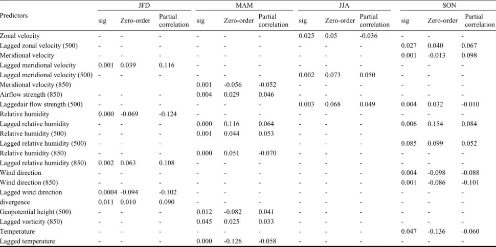
Potential Pre Before buildi nfall, it is imp iables which died region a ationship. Tab sonal rainfall umn. The add s tested using tial and zero odness-of-fit b The key vari

wn to be im ermining rain ength at differ ight Pascal” sons except s ocity, at the s be important p d summer m ection play an d winter mont hough it is c uld be due to ion. The effec

at North-Eas

d Discussio

edictors

ing the ANN portant to sc h influence th and hence fo ble 1 displays l models of w dition of each a stepwise pr correlations, based on sign iable such a mportant pred nfall. Relativ rent levels (su ) are shown summer and w surface or 500 predictor of r months. Whil n important ro hs, this effect characterized o inclusion of ct of correlati st of Iraq

n

N regression reen the suit he rainfall fe orm predictor s the main pre winter, spring, h new predicto rocedure and a measure o nificance. as meridional dictor for al ve humidity urface, 500 hp n to be imp winter respec 0 hPa level, w rainfall during e temperatur ole for the au t was not foun

with warm f effect of al ion for geopo

n model for able climatic eature in the r-predictands edictors in the , summer and or to a model assessing the of the relative l velocity is ll seasons in and airflow p and 850 hp ortant in all ctively. Zonal would appear g the autumn re and wind utumn, spring nd in summer weather that ltitude in the tential height r c e s e d l e e s n w p l l r n d g r t e t

(6)

Table 1 Selected climate variable (predictors). Predictors

JFD MAM JJA SON

sig Zero-order Partial _correlation sig Zero-order Partial _correlation sig Zero-order Partial _correlation sig Zero-order Partial _correlation

Zonal velocity - - - 0.025 0.05 -0.036 - - -

Lagged zonal velocity (500) - - - 0.027 0.040 0.067

Meridional velocity - - - 0.001 -0.013 0.098

Lagged meridional velocity 0.001 0.039 0.116 - - - - - -

Lagged meridional velocity (500) - - - - 0.002 0.073 0.050 - - -

Meridional velocity (850) 0.001 -0.056 -0.052 - - - - - -

Airflow strength (850) - - - 0.004 0.029 0.046 - - - - - -

Laggedair flow strength (500) - - - 0.003 0.068 0.049 0.004 0.032 -0.010

Relative humidity 0.000 -0.069 -0.124 - - - - - -

Lagged relative humidity - - - 0.000 0.116 0.064 - - - 0.006 0.154 0.084

Relative humidity (500) - - - 0.001 0.044 0.053 - - -

Lagged relative humidity (500) - - - 0.085 0.099 0.052

Relative humidity (850) - - - 0.000 0.051 -0.070 - - - - - -

Lagged relative humidity (850) 0.002 0.063 0.108 - - - - - -

Wind direction - - - 0.004 -0.098 -0.088

Wind direction (850) - - - 0.001 -0.086 -0.101

Lagged wind direction 0.0004 -0.094 -0.102 - - - - - -

divergence 0.011 0.010 0.090 - - -

Geopotential height (500) - - - 0.012 -0.082 0.041 - - - - - -

Lagged vorticity (850) - - - 0.045 0.025 0.033 - - - - - -

Temperature - - - 0.047 -0.136 -0.060

(7)

at 500 and vorticity at 850 was captured in spring only. Table 1 shows ranges of significant correlation between 0.013-0.136 and 0.01-0.124 for zero and partial correlation respectively with significant level of less than 5% which results in number of selected predictors ranged between 3-8 predictors across the four seasons.

5.2 Rainfall Model Feature and Efficiency

To adequately assess the ability of the ANN technique employed to capture the underlying relationships between the large-scale atmospheric predictors and rainfall, the data were split into three periods, one for calibration & validation and that applied during the training process and another set for independent verification purposes after the training terminate. The validation period is normally applied for ANN during the training to monitor the training error in order to avoid the over fitting. The calibration and validation periods for the four seasonal models were selected randomly within the period 1980-2001. Different percentages have been tested to investigate the suitable ratio which results in 80% of the data were selected for calibration, 5% for validation and 15% for verification. When calibrating the ANN, outliers were

found to have a large impact on the resulting models and were excluded from subsequent analysis.

Structures of the neural networks used in building the models are shown in Fig. 4. It can be deduced from the network structures in Fig. 4 that the ANN modelling approach employs a larger number of neurons in the hidden layers for all seasons. This larger number of neurons in the hidden layers generally contributes to the accuracy of the model and was selected based on the size of the input layer and ability of the model to perform well in term of ANN performance function (RMSE).

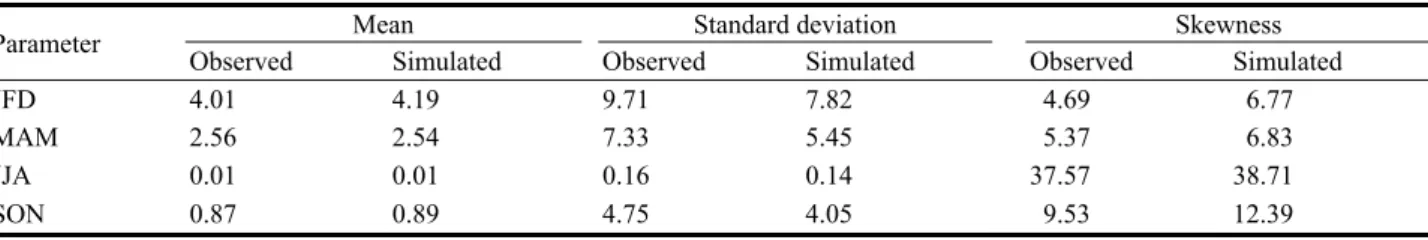
Table 2 shows results of the model produced from ANN against the observed data for each season in respect of mean, standard deviation and skewness. Generally, all the fitted seasonal models perform well, as they reproduce the mean exactly. Nevertheless, looking at the model results in terms of standard deviation and skewness, there is some over/underestimation respectively across the whole seasons. This can be attributed to the fact that study area has the high rainfall variability and skewness (intense rainfall) due to the location in the mountainous area.

Figs. 5 and 6 show the comparison between monthly

Fig. 4 Structure of ANN for (a) winter, (b) spring, (c) summer and (d) autumn models which were trained with back propagation alogrith using sigmoid and linear functions in the hidden and output layer.

Table 2 Statistics of model-computed versus observed daily rainfall for years 1980-2001.

Parameter Mean Standard deviation Skewness

Observed Simulated Observed Simulated Observed Simulated

JFD 4.01 4.19 9.71 7.82 4.69 6.77 MAM 2.56 2.54 7.33 5.45 5.37 6.83 JJA 0.01 0.01 0.16 0.14 37.57 38.71 SON 0.87 0.89 4.75 4.05 9.53 12.39 (a) (b) (c) (d)

(8)

Fig. 5 Average monthly rainfall of the observed and simulated rainfall during calibration and verification periods (1980-2001).

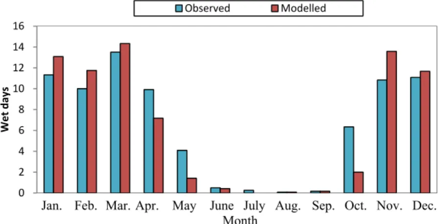
Fig. 6 Average monthly numbers of wet days of the observed and simulated rainfall during calibration and verification periods (1980-2001).

rainfall for both the observed and modelled series for the calibration and verification periods (1980-2001) which demonstrate a good degree of correspondence. The visual plot in Fig. 6 shows the monthly average wet days for the observed and modelled rainfall for calibration and verification periods. The plot shows that the model is slightly over and under estimate the rainfall for some months by up to 2 days which demonstrated that ANN is a good choice for downscaling future rainfall. This would entail the assumption that model parameters are assumed time invariant and would not change in future. So both monthly pattern (wet days and rainfall) would appear to have been adequately captured by the model, an important requirement when assessing climate impacts on such systems as the hydrological system.

Furthermore, quantile-quantile plots [35] of the four

seasons were used to assess the model performance by comparing the simulated rainfall against the observed one after arranged in ascending order (Fig. 7). As seen in Fig. 7, model bias was found for most storm events for the four seasons. The model output-driven rainfall prediction was a bit lower than the actual observation. A reason for this discrepancy might be explained by the converse behavior of altitudinal dependence of precipitation between actual observation and that obtained from model outputs.

Ability of the seasonal models in reproducing the current climate was also evaluated using correlation coefficient (R), Nash coefficient (Nash) [36], RMSE (root mean squared error) [37] and Bias [38] as in Figs. 8 and 9. The autumn and summer months appear to produce the best results as represented with high the correlation and Nash coefficient of 0.88 & 0.89 and 0 20 40 60 80 100 120 140 160 Rain fall (mm) Observed Modelled 0 2 4 6 8 10 12 14 16 Wet da ys Observed Modelled

Jan. Feb. Mar. Apr. May June July Aug. Sep. Oct. Nov. Dec.

Month

Jan. Feb. Mar. Apr. May June July Aug. Sep. Oct. Nov. Dec.

(9)

(a) (b)

(c) (d)

Fig. 7 Quantile-quantile plot for observed and simulated daily rainfall for (a) winter, (b) spring, (c) summer and (d) autumn during calibration and verification periods (1980-2001).

Fig. 8 ANN model efficiency in terms of R and Nash during calibration and verification periods (1980-2001).

Fig. 9 RMSE and Bias for calibration and verification periods (1980-2001) for the four seasons. 0 20 40 60 80 100 120 140 0 20 40 60 80 100 120 140 Mo del le d(mm) 0 20 40 60 80 100 0 20 40 60 80 100 Mod e lled (mm) 0 1 2 3 4 5 6 7 8 0 2 4 6 8 Mod e lled (mm) 0 20 40 60 80 100 0 20 40 60 80 100 Mod e lled (mm) 0 0.2 0.4 0.6 0.8 1

JFD MAM JJA SON

Efficien cy R Nash ‐6 ‐4 ‐2 0 2 4 6 8 10

JFD MAM JJA SON

Erro r (%) RMSE Bias Observed Observed Observed Observed

(10)

0.77% & 0.79, respectively. As results the Bias and

RMSE were quite low in order of 3% and 2% as a

maximum. However, all results are comparable between seasons and the correlation between day to day variability does not go below 0.60 with corresponding efficiency of 0.42, Bias 4.6% and RMSE 7.5% as a minimum and that was associated with the winter season.

Extreme rainfall is considered one of the most important parameters used in the design of many hydrological systems. So the ability of the ANN model to reproduce extreme values of rainfall has also been assessed in this study using a combined approach of annual maximum and GEV (generalised extreme value) distribution [39]. Fig. 10 shows an example of the CDF (cumulative distribution function) for the observed and simulated extremes (daily) rainfall at Iraq in the winter, spring, summer and autumn seasons. It can be observed in Figs. 10a-10d that the cumulative distribution function produced by the ANN model closely matches

or exceeds the corresponding observed one for extreme rainfall at daily scale at all seasons. The conclusion that can be made from cumulative distribution function plots is that the ANN model is reasonable in representing extreme rainfall observations and their probability.

5.3 Scenarios of Future Rainfall Projection up to 21st Century

Once the downscaling models have been calibrated and validated, the next step is to use these models to downscale the control scenario and future scenario simulated by the GCM (HadCM3). Synthetic daily rainfall time series were produced for HadCM3 A2 for a period of 139 years (1961-2099). The outcome was divided by three periods of time, which are 2020s (2010-2039), 2050s (2040-2069) and 2080s (2070-2099). Climate change was assessed by comparing these three future time slices with baseline period of 1961-1990 as recommended by the Intergovernmental Pannel of Climate Change.

(a) (b)

(c) (d)

Fig. 10 CDFs of model-computed versus observed daily extremes rainfall for (a) JFD, (b) MAM, (c) JJA and (d) SON for years 1980-2001. 0 0.2 0.4 0.6 0.8 1 0 50 100 150 Prob ab ility Observed Modelled 0 0.2 0.4 0.6 0.8 1 0 20 40 60 80 100 120 Prob ab ility Observed Modelled 0 0.2 0.4 0.6 0.8 1 0 2 4 6 8 Prob ab ility Observed Modelled 0 0.2 0.4 0.6 0.8 1 1.2 0 20 40 60 80 100 Prob ab ility Observed Modelled Extreme (mm) Extreme (mm) Extreme (mm) Extreme (mm)

(11)

Trend study for observed rainfall data is widely used as a base reference or a caveat of climate change studies [40]. Also, it can provide a quick visual check for the presence of unreasonable values (outliers). However, the usefulness of trend study is always being questioned as the these trends depend on the accuracy of the observed data. Possible trends in the data are investigated to offer an historical context before further climate change assessments in this work.

Using a simple linear trend approach [41], the gradient and its variance of the resulting regression of the hydrological series with respect to time is used to check the possible trends in the rainfall series. Based on the Wald statistics, the significance of trend gradients is tested based on a normally distributed assumption (significant level is 5%). Hannaford and Marsh [41] used a similar linear regression approach to look at runoff trends in UK. Fig. 11 shows series plots and their trend lines for the average annual rainfall for which show a significant downward trend for both A2 and B2 scenarios for the period 1961-2099 with acute trend for A2 scenario and that indicate climate change

did take place since the observed period data.

Fig. 12 presents average monthly rainfall simulated by HadCM3 GCM for A2 and B2 scenarios of greenhouse emission for the three future periods compared with the baseline period. Both plots consistently project some reduction in the monthly rainfall for the 2020s, 2050s and 2080s; however, 2080s experience largest drop especially during April (0.51%) and July (77%) months of A2 and during May (49%) and July (79%) of B2. Generally, the projected rainfall in future varies significantly/slightly amongst the three future periods and the emission scenario considered as A2 experience more significant reduction than scenario B2.

Other comparative plots of future periods against the baseline period are the daily rainfall box plots of the four seasons of A2 and B2 scenarios which were presented in Fig. 13. The daily rainfall box plots are different across all seasons for the entire statistics while mix projections were found within the future periods. While the winter projects some increase/decrease in the daily rainfall statistics of wet days (maximum, 3rd quantile,

(a)

(b)

Fig. 11 Average annual rainfall for (a) A2 scenario and (b) B2 scenario compared with control period. 0 200 400 600 800 1000 1200 1960 1980 2000 2020 2040 2060 2080 2100 Rain fall (mm) 0 200 400 600 800 1000 1200 1960 1980 2000 2020 2040 2060 2080 2100 Rain fall (mm) Year Year 1,200 1,000 800 600 400 200 0 1,200 1,000 800 600 400 200 0

(12)

(a)

(b)

Fig. 12 Average monthly rainfall for (a) A2 and (b) B2 scenarios relative to baseline period.

(a)

(b)

Fig. 13 The daily rainfall box plots across the four seasons for different future periods of (a) A2 and (b) B2 scenarios compared with baseline period.

0 20 40 60 80 100 120 140 160 0 1 2 3 4 5 6 7 8 9 10 11 12 Rain fall (mm) Basline 2020s 2050s 2080s 0 20 40 60 80 100 120 140 160 0 1 2 3 4 5 6 7 8 9 10 11 12 Rain fall (mm) Basline 2020s 2050s 2080s 0 5 10 15 20 25 30 35 40 45 Rain fall (mm)

JFD MAM JJA SON

0 5 10 15 20 25 30 35 40 45 Rain fall (mm) JFD _MAM JJA SON Month Month

(13)

mean, 1st quantile and minimum), the spring season show between very slight drop and no change for both scenarios. However, both summer and autumn show a significant reduction in maximum rainfall value especially in 2080s while the other statistics remain nearly the same. In term of mean daily rainfall, a drop up to 8%, 6% and 24% for winter, spring and autumn respectively can be detected for A2 scenario by 2080s, while B2 projects a maximum drop of up to 6%, 10%, 48% and 18% for winter, spring, summer and autumn.

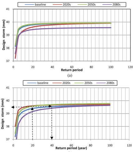
Moreover, analysis for the obtained quantiles simulated by GEV revealed changes in the intensity and frequency (return period) of the extreme rainfall in the future periods of the 2020s, 2050s and 2080s for scenario A2 and B2 compared to the extreme rainfall derived from the observed baseline period 1961-1990 as in Fig. 14. The extremes events are projected to decrease slightly in 2080s with highest decrease

associated with A2 scenario. This is because the rainfall under scenario A2 is more significant than under scenario B2 (the IPPC assumption is that CO2 concentration is higher in A2 than B2). So that causes the temperature to be very high with increase in emission scenario leading to more water vapor and in turn more rainfall.

The 2020s and 2050s showed no considerable change across the different return periods for A2 and B2 especially with the higher return period while the lower periods show some increase and decrease. The results obtained from the extreme analysis of rainfall in the future periods under climate change clearly demonstrate that in general future extreme rainfalls are projected to be less frequent especially in 2080s while a very small drop is detected (up to 2%) due to location of the study area in mountain region. The return period of a certain rainfall will increase in the future as

(a)

(b)

Fig. 14 Future daily rainfall extremes for different return period of (a) A2 and (b) B2 scenarios compared with baseline period. 37 38 39 40 41 0 20 40 60 80 100 120 Design storm (mm) Return period baseline 2020s 2050s 2080s 37 38 39 40 41 0 20 40 60 80 100 120 Design storm (mm) Return period (year) baseline 2020s 2050s 2080s

(14)

demonstrated by the dashed line for quantile-return period plot displayed in Fig. 14 when a present storm of 20 year could occur once every 43 year in the 2080s. The results in Fig. 14 also show that an increase in the frequency of extreme rainfall varies between the future periods and the emission scenarios considered.

6. Conclusions

Iraq is facing water shortage problems. In this research, rainfall records were investigated in the northeast part of Iraq to analyze the expected future rainfall trends. Rainfall records of Sulaimani city were used in two scenarios—A2 and B2. The results indicate that the average annual rainfall shows a significant downward trend for both A2 and B2 scenarios for the period 1961-2099 with acute trend for A2 scenario and that indicate climate change did take place since the observed period data. Average monthly rainfall simulated by HadCM3 GCM for A2 and B2 scenarios of greenhouse emission for the three future periods compared with the baseline period show some reduction in the monthly rainfall for the 2020s, 2050s and 2080s; however, 2080s experience largest drop especially during April and July months of A2 (51% and 77%) and during May and July of B2 (49% and 79%) .

Generally, the projected rainfall in future varies significantly/slightly amongst the three future periods and the emission scenario considered as A2 experience more significant reduction than scenario B2.

Moreover, analysis for the obtained quantiles simulated by GEV revealed changes in the intensity and frequency (return period) of the extreme rainfall in the future periods for scenario A2 and B2 compared to the extreme rainfall derived from the observed baseline period. The extremes events are to decrease slightly in 2080s with highest decrease associated with A2 scenario. This is because the rainfall under scenario A2 is more significant than under scenario B2. The 2020s and 2050s showed no considerable change across the different return periods for A2 and B2 especially with

the higher return period while the lower periods show some increase and decrease.

Acknowledgments

The authors would like to thank Mrs. Semia Ben Ali Saadaoui of the UNESCO-Iraq for her encouragement and support. Thanks to Sulaimani University for providing some related data. The research presented has been financially supported by Luleå University of Technology, Sweden and by “Swedish Hydropower Centre-SVC” established by the Swedish Energy Agency, Elforsk and Svenska Kraftnät together with Luleå University of Technology, The Royal Institute of Technology, Chalmers University of Technology and Uppsala University. Their support is highly appreciated.

References

[1] N.A. Al-Ansari, Water resources in the Arab countries: Problems and possible solutions, in: UNESCO (United Nations Educational, Scientific and Cultural Organization) International Conference (Water: A Looming Crisis), Paris, France, 1998, pp. 367-376.

[2] F. Salem, Water sustainability—A national security issue for the middle east and north Africa region, in: 2nd International Water Conference in the Arab Countries, France, July 7-10, 2003.

[3] M.K. Tolba, O.A. El-Khouly, K.A. Thabet, The Future of Environmental Action in the Arab World, UNEP/Environment Agency Abu Dhabi, 2001. (in Arabic)

[4] M. Kassa, Aridity, drought and desertification, in: M. Tolba, N. Saab (Eds.), Arab Environment and Future Challenges, Chapter 7, The Arab Forum for Environment and Development, Egypt, 2008.

[5] T. Naff, Conflict and water use in the Middle East, in: R. Roger, P. Lydon (Eds.), Water in the Arab Word: Perspectives and Prognoses, Harvard University, 1993, pp. 253-284.

[6] N.A. Al-Ansari, Applied Surface Hydrology, Al Al-Bayt University Publication, Al Al-Bayt University Press, 2005.

[7] F. Bazzaz, Global climatic changes and its consequences for water availability in the Arab World, in: R. Roger, P. Lydon (Eds.), Water in the Arab Word: Perspectives and Prognoses, Harvard University, 1993, pp. 243-252. [8] K. Voss, J. Famiglietti, M. Lo, C. de Linage, M. Rodell, S.

(15)

Swenson, Groundwater depletion in the Middle East from GRACE with implications for transboundary water management in the Tigris-Euphrates-Western Iran region, Water Resources Research 49 (2013) 904-914.

[9] N.A. Al-Ansari, Management of water resources in Iraq: Perspectives and prognoses, Journal Engineering 5 (2013) 667-684.

[10] B.O. Elasha, Mapping of Climate Change Threats and Human Development Impacts in the Arab Region, United Nations Development Programme, Arab Human Development report (AHDR), Research Paper Series, 2010. [11] IPCC (Intergovernmental Panel on Climate Change), Climate Change Impacts, Adaptation and Vulnerability, Cambridge University Press, Geneva, 2007.

[12] P.C.D. Milly, K.A. Dunne, A.V. Vecchia, Global patterns of trends in streamflow and water availability in a changing climate, Nature 438 (2005) 347-350.

[13] N.A. Al-Ansari, S. Knutsson, Toward prudent management of water resources in Iraq, Journal of Advanced Science and Engineering Research 1 (2011) 53-67.

[14] Water Resources Management White Paper, United Nations Assistance Mission for Iraq, United Nations Country Team in Iraq, United Nations, 2010.

[15] N.A. Al-Ansari, E. Salameh, I. Al-Omari, Analysis of Rainfall in the Badia Region, Jordan, Al Al-Bayt University Research Paper No. 1, 1999, p. 66.

[16] N.A. Al-Ansari, B. Al-Shamali, A. Shatnawi, Statistical analysis at three major meteorological stations in Jordan, Al Manara Journal for Scientific Studies and Research 12 (2006) 93-120.

[17] N.A. Al-Ansari, S. Baban, Rainfall trends in the Badia region of Jordan, Surveying and Land Information Science 65 (4) (2005) 233-243.

[18] E. Kalnay, M. Kanamitsu, R. Kistler, W. Collins, D. Deaven, L. Gandin, et al., The NCEP/NCAR 40-year reanalysis project, Bulletin of the American Meteorological Society 77 (3) (1996) 437-471.

[19] C.J. Willmott, C.M. Rowe, W.D. Philpot, Small-scale climate map: A Sensitivity analysis of some common assumptions associated with the grid-point interpolation and contouring, American Cartographer 12 (2) (1985) 5-16.

[20] D.A. Shannon, B.C. Hewitson, Cross-scale relationships regarding local temperature inversions at cape town and global climate change implications, South African Journal of Science 92 (4) (1996) 213-216.

[21] R.G. Crane, B.C. Hewitson, Doubled CO2 precipitation

changes for the Susquehanna basin: Down-scaling from the genesis general circulation model, International Journal of Climatology 18 (1) (1998) 65-76.

[22] F. Giorgi, L.O. Mearns, Approaches to the simulation of

regional climate change, Reviews Geophysics 29 (1991) 191-216.

[23] T.M.L. Wilby, D. Wigley, P.D. Conway, B.C. Jones, J.M. Hewitson, D.S. Wilks, Statistical downscaling of general circulation model output: A comparison of methods, Water Resources Research 34 (1998) 2995-3008.

[24] C. Harpham, R.L. Wilby, Multisite-downscaling of heavy daily precipitation occurrence and amounts, Journal of Hydrology 312 (2005) 1-21.

[25] M. Abdellatif, W. Atherton, R. Alkhaddar, Climate change impacts on the extreme rainfall for selected sites in north western England, Open Journal of Modern Hydrology 2 (3) (2012) 49-58.

[26] N.D. Hoai, K. Udo, A. Mano, Downscaling global weather forecast outputs using ANN for flood prediction, Journal of Applied Mathematics 2011 (2011) 1-14.

[27] CCIS (Canadian Climate Impacts Scenarios Group)[Online], 2010, http://www.cics.uvic.ca/scenarios/ index.cgi?More_Info-SDSM_Background (accessed Jan. 1, 2014).

[28] S. Haykin, Neural Networks: A Comprehensive Foundation, MacMillan, New York, 1994.

[29] K.L. Hsu, H.V. Gupta, S. Sorooshian, Artificial neural network modelling of the rainfall-runoff process, Water Resources Research 31 (10) (1995) 2517-2530.

[30] R.S. Govindaraju, A.R. Rao, Artificial Neural Networks in Hydrology, Kluwer, The Netherlands, 2000.

[31] K. Levenberg, A method for the solution of certain problems in least squares, Quarterly of Applied Mathematics 5 (1944) 164-168.

[32] D. Marquardt, An algorithm for least-squares estimation of nonlinear parameters, SIAM Journal on Applied Mathematics 11 (2) (1963) 431-441.

[33] R.M. Trigo, Improving metrological downscaling methods with artificial neural network models, Ph.D. Thesis, University of East Anglia, 2000.

[34] CCIS (Canadian Climate Impacts Scenarios Group) [Online], http://www.cics.uvic.ca/scenarios/index.cgi? More_Info-Baseline_Climate (accessed Jan. 29, 2013). [35] M. Abdellatif, Modelling the impact of climate change on

urban drainage systems, Ph.D. Thesis, Liverpool John Moores University, 2013.

[36] J.E. Nash, J.V. Sutcliffe, River flow forecasting through conceptual models, Part I—A discussion of principles, Journal of Hydrology 10 (1970) 282-290.

[37] M.G. Schaap, F.J. Leij, Database related accuracy and uncertainty of pedotransfer functions, Soil Science 16 (1998) 765-779.

[38] H.V. Gupta, S. Sorooshian, P.O. Yapo, Status of automatic calibration for hydrologic models: Comparison with multilevel expert calibration, Journal of Hydrologic Engineering 4 (1999) 135-143.

(16)

Climate Change and Future Long-Term Trends of Rainfall at North-East of Iraq 805 [39] S. Coles, An Introduction to Statistical Modelling of

Extreme Values, Springer Series in Statistic, London, 2001.

[40] G. Jenkins, M. Perry, G. Prior, The Climate of the United Kingdom and Recent Trends, Met Office Hadley Centre,

UK, 2009.

[41] J. Hannaford, T. Marsh, An assessment of trends in UK runoff and low flows using a network of undisturbed basins, International Journal of Climatology 26 (9) (2006) 1237-1253.