Self-Stabilizing Platform Självstabiliserande serveringsbricka

IN

DEGREE PROJECT TECHNOLOGY, FIRST CYCLE, 15 CREDITS

, STOCKHOLM SWEDEN 2020

Self-Stabilizing Platform

Självstabiliserande

serveringsbricka

MARCUS AKKILA

BIX ERIKSSON

Self-Stabilizing Platform

MARCUS AKKILA BIX ERIKSSON

Bachelor’s Thesis at ITM Supervisor: Nihad Subasic

Abstract

This project explores the possibility to stabilize a hand held serving-tray using a micro-controller, two servomo-tors and an inertial measurement unit (IMU). It is heav-ily focused on control theory, specifically using a PID con-troller. Stabilization of an object using a PID controller have many applications such as drones, camera stabilizers and flight simulators. The report covers the theory neces-sary to construct a self stabilizing platform and describes involving components in the prototype and how they coop-erate. With the gyroscopes and accelerometers involved in the IMU it is possible to determine orientation and rota-tion of the tray. The construcrota-tion enables rotarota-tion about the x-axis (roll) and y-axis (pitch) but not the z-axis (yaw). The readings from the gyroscopes and the accelerometers are combined and filtered through a complementary filter to estimate the rotations. The servomotors compensate dis-turbance in keeping the platform horizontal through PID regulation. The PID constants are tuned through tilting the platform at a specific angle and plotting the step re-sponse in MATLAB.

Referat

Självstabiliserande serveringsbricka

Detta projekt utforskar m¨ojligheten att stabilisera en handh˚allen serveringsbricka med hj¨alp av en mikrokontrol-ler, tv˚a servomotorer och en tr¨oghetssensor (IMU). Pro-jektet l¨agger mycket fokus p˚a reglerteknik, specifikt att anv¨anda en PID-regulator. Stabilisering genom PID-reglering ¨ar anv¨andbart i m˚anga olika produkter, exempelvis dr¨onare, kamerastabiliserare och flygsimulatorer. Rapporten t¨acker relevant teori f¨or att konstruera en sj¨alvstabiliserande platt-form och beskriver ing˚aende komponenter i prototypen samt hur de samverkar. Med gyroskopen och accelerometrarna som finns i IMU:n ¨ar det m¨ojligt att uppskatta position och rotation f¨or ett objekt. Konstruktionen till˚ater rota-tion kring x-axeln (roll) och y-axeln (pitch) men inte z-axeln (yaw). M¨atningarna fr˚an gyroskopen och accelero-metrarna kombineras och filtreras med hj¨alp av ett s.k. complementary filter f¨or att uppskatta rotationen av ob-jektet. Servomotorerna anv¨ands i sin tur till att h˚alla plat-tan horisontell genom att kompensera st¨orningar fr˚an om-givningen. Detta g¨ors genom PID-reglering. Konstanterna i PID-regulatorn ¨ar framtagna genom tester d¨ar plattfor-men lutas ett best¨amt antal grader och stegsvaret plottas i MATLAB.

Nyckelord: Mekatronik, PID-regulator, Reglerteknik, Ar-duino, Servomotor, Tr¨oghetssensor, Sj¨alvstabilsering

Acknowledgements

We would especially like to thank Seshagopalan Thorapalli Muralidharan for helping us throughout this project. He has been available regardless of the time of day. We had several components that broke close to the deadline and he supplied us with new components within 24 hours. A thank you to Staffan Qvarnstr¨om for supplying us with the electronic components. We would also like to thank Nihad Subasic, course

Contents

1 Introduction 1 1.1 Background . . . 1 1.2 Purpose . . . 2 1.3 Method . . . 2 1.4 Scope . . . 3 2 Theory 5 2.1 Inertial Measurement Unit (IMU) . . . 5

2.2 Filtering Disturbances . . . 5

2.2.1 Complemantary Filter . . . 5

2.3 Calculating Roll and Pitch Angles Using Accelerometers . . . 6

2.4 PID controller . . . 8

2.4.1 Servomotors and PWM . . . 9

2.5 Microcontroller . . . 10

2.6 Mathematical Model . . . 10

3 Materials and Design 13 3.1 Design . . . 13

3.2 The TowerPro SG-5010 Servomotor . . . 13

3.3 The Inertial Measurement Unit LSM6DS3 by SparkFun . . . 14

3.4 Electrical Circuit . . . 15

3.5 Controller for the Platform . . . 16

3.6 The Code for the Platform . . . 16

4 Results 19 4.1 PID response without weight distribution . . . 19

4.2 PID response with weight distribution . . . 23

5 Discussion 25

6 Conclusion 27

Bibliography 31

Appendices 32

A Arduino Code 33

List of Figures

1.1 A Stewart Platform [2] . . . 1

1.2 Experimental setup, made in Adobe illustrator[4] . . . 3

2.1 Complementary filter made in paint . . . 6

2.2 Orientation of the serving tray, made in Adobe illustrator[4] . . . 7

2.3 Block diagram showing the implementation of a PID-controller in a sys-tem[13]. . . 9

2.4 Different duty cycles [14] . . . 10

2.5 Servomotor connected to tray made in Paint . . . 11

2.6 Tilting tray made in Paint . . . 12

3.1 Design of the platform made in Solid Edge ST9[15] . . . 13

3.2 Servomotors used in the prototype[17] . . . 14

3.3 Inertial measurement unit used in the prototype[18] . . . 14

3.4 Circuit diagram made in Fritzing[20] . . . 15

3.5 Flowchart over how the code for the platform works, made in draw.io[21] 17 4.1 Kp = 4, Ki = 0, Kd= 0 . . . 20

4.2 Kp = 1.35, Ki = 0.57, Kd= 0 . . . 21

4.3 Kp = 1.35, Ki = 0.57, Kd= 0.08 . . . 22

4.4 250 gram weight Kp = 1.35, Ki = 0.57, Kd= 0.08 . . . 23

List of Abbreviations

IMU Inertial Measurement Unit PID Proportional-Integral-Derivative CAD Computer Aided Design

PWM Pulse Width Modulation CPU Central Processing Unit DC Direct Current

Chapter 1

Introduction

1.1

Background

An inspiration for this project was the advanced platform type called the Stew-art Platform. A StewStew-art Platform uses six motors to be able to balance objects on it. It can detect position and motion of the object using sensors, and then compensate the motion by using its motors to make adjustments in six degrees of freedom. Figure 1.1 shows a Stewart platform made by Acrome Robotics. With good equipment it can react very fast and with great precision. The first Stew-art Platform was presented in 1965 in form of a flight simulator[1]. It is now widely used in industries such as aerospace, nautical and automotive technology.

Figure 1.1. A Stewart Platform [2]

To stabilize an object using control systems is a classic implementation of mecha-tronics. Useful applications include drones, gimbals for cameras and spoons that

CHAPTER 1. INTRODUCTION

keep themselves horizontal. A gimbal is a support that allows rotation about an axis. The 3-axis camera gimbal is a handheld mount for the camera which uses three motorized gimbals to compensate for any disturbances in keeping the camera stable. Algorithms and sensors are used to calculate how much the motors must rotate to cancel out any unwanted movement. Self stabilizing spoons can be used by people with diseases that causes hand tremors such as Parkinson’s disease. This simplifies the eating process a lot for these people[3].

1.2

Purpose

The serving tray is to be used in restaurants were drinks are to be served quick, without spilling any of the liquid. The research questions for this project are:

1. How do we use the information from the inertial measurement unit (IMU) to stabilize the platform?

2. How will variations in PID constants affect the performance in regards to speed regulations and smoothness?

3. How will differences in load and weight distribution affect the PID-controller?

1.3

Method

The prototype is built up by servomotors, a microcontroller of type Arduino Uno and an inertial measurement unit of type LSM6DS3. These are used to keep the serving tray horizontal when walking with it. The servomotors are placed on top of a base platform perpendicular to each other. These are used to control the angle of a platform (the serving tray) on top of the base platform. A pole with a ball joint is used in the middle of the platform to support the servomotors.

1.4. SCOPE

A PID controller has been implemented to govern the stabilization of the plat-form.

Figure 1.2. Experimental setup, made in Adobe illustrator[4]

The performance of the PID has been analyzed by introducing a step-response to the system. The step-response in this case consists of tilting the tray from an horizontal position, which in turn will create an angle offset error, α, as seen in figure 1.2. The PID controller will then try to compensate this disturbance. The PID response has been registered and plotted using MATLAB[5]. The aim of the test is to see how the P, I and D parts of the controller work together to stabilize the platform, and how this relationship change when a weight distribution is added.

1.4

Scope

The project will involve a prototype and a report. The purpose of this project is to produce a self-stabilizing platform with simplicity and low cost. The prototype will be produced with a budget of 1000 SEK. A Stewart platform can move freely with six degrees of freedom. The platform in this project will be able to rotate about the x-axis and y-axis but not around the z-axis, what is typically called the yaw rotation. Necessary theory needed to construct this platform will be covered in the theory chapter.

Chapter 2

Theory

2.1

Inertial Measurement Unit (IMU)

An inertial measurement unit is an electronic sensor that is placed on a body in order to determine where and how it is moving. The IMU detects linear accelera-tion using accelerometers and rotaaccelera-tional rate using gyroscopes. One accelerometer, gyroscope and magnetometer for each vehicle axis is a common configuration. The magnetometer is used as a heading reference[6]. The IMU allows tracking of a body’s speed, acceleration, turn rate and inclination. It is therefore commonly used for navigational purposes. In aircrafts, where it is highly necessary to track changes in attitude, it is an essential component.

2.2

Filtering Disturbances

When using an IMU a problem arises when trying to combine the accelerometer and gyroscope data. Both are used for the same purpose, to get the angular position of the object. Some data will cause disturbances in the system and therefore the data should be filtered in order to gather information about the actual state of the system. The powerful recursive filter called Kalman filter is useful when the information received from a dynamic system is unpredictable. Therefore it might seem suitable for this application, but it is far too complex. A complementary filter is most likely more appropriate.

2.2.1 Complemantary Filter

A complementary filter is a steady state Kalman filter for a certain class of filtering problems[7]. When it is applied on the values received from the IMU it evaluates an estimated angular position by mostly using the information received from the gyroscope, but also some from the accelerometers. The data received from the gyroscope will be valued higher in the estimation because it is more accurate and does not suffer from external forces. The downside of the gyroscope is that it drifts,

CHAPTER 2. THEORY

meaning that it introduces error in the output as time passes[8]. The complementary filter can therefore be implemented to get a more accurate estimation of the roll and pitch angles. It cannot be used to calculate yaw since the accelerometers does not give any data about the yaw (the reason for this is explained in chapter 2.3). The yaw can therefore only be estimated using the gyroscope when a six degrees of freedom IMU is used.

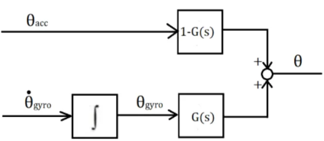
A low pass filter is used to filter short term accelerometer fluctuations and a high pass filter is used to negate the drift of the gyroscope. Figure 2.1 shows how θ (roll or pitch) is calculated. θg y r o is the gyroscopic value and it is a high frequency signal passing through a low pass filter G(s). θacc is the accelerometer value, a low frequency signal passing through a high pass filter 1-G(s).

θacc(1 − G(s)) + θg y r oG(s) = θ (2.1)

Figure 2.1. Complementary filter made in paint

The theory behind this is that the noise in the high frequency signal is mostly low frequency. It should therefore be filtered with a low pass filter G(s)[7]. The opposite applies to the low frequency signal.

2.3

Calculating Roll and Pitch Angles Using

Accelerometers

The orientation of the tray can be described by the pitch, roll and yaw angles of the platform and it is essential for the project to accurately calculate these angles. The calculation of the angles is done through the accelerometers on the IMU which measure acceleration in the unit g (gravitational acceleration). When measuring orientation in the earth’s gravitational field, the accelerometers should be calibrated so that one of the accelerometers gives the value +1g when an axis is aligned with the earth’s gravitational field. Let a be the linear acceleration of the object and Gp be the vector containing the measurements from the accelerometers, then:

Gp =    Gpx Gpy Gpz   = R(g − ar) (2.2) 6

2.3. CALCULATING ROLL AND PITCH ANGLES USING ACCELEROMETERS

Figure 2.2. Orientation of the serving tray, made in Adobe illustrator[4]

where R is the rotation matrix describing the orientation of the object relative to the earth’s coordinate frame.

When aligning the object so that the roll, pitch and yaw angles represent rotation about the x, y and z axis respectively as seen in figure 2.2, the rotation matrices will be as follows[9]: Rx(φ) =    1 0 0 0 cos(φ) sin(φ) 0 −sin(φ) cos(φ)    (2.3) Ry(θ) =    cos(θ) 0 −sin(θ) 0 1 0 sin(θ) 0 cos(θ)    (2.4) Rz(ψ) =    cos(ψ) sin(ψ) 0 −sin(ψ) cos(ψ) 0 0 0 1    (2.5)

These can be used to transform a vector under rotation. This is useful when transforming the earth’s gravitational field vector to determine the position of an

CHAPTER 2. THEORY

object. By aligning the z-axis with the earth’s gravitational field (+g for z), defining the roll, pitch and yaw as in figure 2.2 and also assuming no linear acceleration (from vibrations etc.) the transformation becomes[9]:

Rxy z    0 0 1   = Rx(φ)Ry(θ)Rz(ψ)    0 0 1   =    −sin(θ) cos(θ)sin(φ) cos(θ)cos(φ)    (2.6)

Equation 2.6 can be rewritten in the form of equation 2.7 by relating the roll and pitch angles to the normalised accelerometer values Gp:

Gp | Gp | =    −sin(θ) cos(θ)sin(φ) cos(θ)cos(φ)   → 1 q Gp2x+ Gp2y+ Gp2z    Gpx Gpy Gpz   =    −sin(θ) cos(θ)sin(φ) cos(θ)cos(φ)    (2.7)

This makes it possible to calculate the roll and pitch angles using:

tan(φ) = Gpy Gpz (2.8) tan(θ) = −Gpx Gpysin(φ) + Gpzcos(φ) = −G_px q Gp2y+ Gp2z (2.9) Equation 2.6 does not include any terms containing the yaw angle, this is the reason why it is not possible to calculate the yaw, pitch and roll by only using accelerometers.

2.4

PID controller

A proportional-integral-derivative controller (PID) is a feedback mechanism imple-mented to control a system. The PID controller is one of the most common types of controller used in industries applications. Investigations and surveys from differ-ent industries show that more than 90 percdiffer-ent of all controllers in these industries are implemented with PID or PI (no derivative term) regulation[10][11]. The PID-controller is based upon using the steady state error:

e(t) = r(t) − y(t) (2.10)

where r is the desired state and y is the current state, to calculate the needed input (e.g. force from an engine) in order to reach a steady state. The input, u(t), is calculated through: u(t) = Kpe(t) + Ki Z t 0 e(t)dt + KD d dte(t) (2.11)

where Kp, Ki and Kdare all non-negative and represent the proportional, inte-gral and derivative terms respectively[12]. Figure 2.3 shows a block diagram over how the PID-controller is implemented.

2.4. PID CONTROLLER

Figure 2.3. Block diagram showing the implementation of a PID-controller in a

system[13].

2.4.1 Servomotors and PWM

A servomotor uses pulse width modulation (PWM) to determine the angular posi-tion of the motors output shaft and they are typically used in applicaposi-tion where high precision is important. The servomotor shaft typically has an operating range that spans between 0 and 180 degrees which makes it a suitable motor for controlling the rods connected to the platform. Speed will also be an important factor to keep the platform close to horizontal at all times. Servos follow a typical torque-speed-curve, i.e. high speed produces low torque and vice versa. The motor selection and controlling has to be done with consideration to ensure that the motor has the cor-rect operating speed while still producing a sufficient torque. The servo is therefore regulated through pulse width modulation (PWM).

The signal to the servo can only be high (5 V) or low (0 V) at any time, but by controlling the time it is either high or low different signals can be sent. This is possible because the voltage regulation reacts quicker than the servomotor can register. The concept duty cycle is frequently used to describe this. Duty cycles tells how much the signal is high in proportion to low in percentage. For example a 75 percent duty cycle indicates that the digital signal is high 75 percent of the time over an interval. The outcome of this is square waves, where 50 percent duty cycles become a perfect square wave. This is illustrated in figure 2.4.

CHAPTER 2. THEORY

Figure 2.4. Different duty cycles [14]

2.5

Microcontroller

A microcontroller is built up by a processor (CPU), memory and I/O peripherals. It can be considered as a small computer and it is an essential part in many hobby projects in the field of mechatronics. Raspberry Pi and Arduino are known manu-facturers of microcontrollers. Microcontrollers have two types of memory: program memory and data memory. The program memory handles the instructions that the CPU processes. The data memory is used for temporary data storage while the program is running. The I/O peripherals are input and output devices that give the microcontroller data from the sensors and produce electrical outputs which control the various devices that are connected to the board.

2.6

Mathematical Model

If the upper platform, the serving tray, of the model was locked horizontally, its motion when the rod from the servomotor pushes the platform upwards could be described by the following mathematical model:

Let l be the length of the arm from the motor and L be the length of the con-nection (rod) from the arm to the upper platform. Also let α be the angle between the connection and the horizontal plane and β the angle between the arm and the vertical plane, as shown in figure 2.5 where the rod is connected to the tray. In figure 2.5, the vertical distance between the arm and the upper platform is:

Lsin(α) (2.12)

2.6. MATHEMATICAL MODEL

When β is zero degrees the distance is:

L+ l (2.13)

The servo motor can be modified to adjust β a certain angle. For each angle that

β decreases, α increases by:

(90 − arccos(l/L))/90 (2.14) If β decreases with x degrees then the vertical distance increases by:

Lsin(α + x(1 − arccos(l/L))/90) − Lsin(α) + lsin(x) (2.15)

Figure 2.5. Servomotor connected to tray made in Paint

A pole is to be used in between the serving tray and the base platform to relieve load of the servo motors. Motion will be allowed by placing it in the middle of the platform and attaching it to the tray using a ball joint. This mathematical model is therefore not sufficient since the serving tray will be locked vertically in the middle of the tray.

When the pole is attached to the middle of the serving tray the platform will follow the motion displayed in figure 2.6 when the arm of the servomotor rotates upward and therefore presses the tray upwards. This will mainly result in a vertical motion for the connection between the arm and the tray, but also some horizontal movement. The crosses in the figure represents the change in position for the rod of the servo.

The difference in vertical position:

Dsin(ϕ) (2.16)

Horizontal:

CHAPTER 2. THEORY

Figure 2.6. Tilting tray made in Paint

For small values for ϕ, the difference in sinus is much greater than the difference for cosine. Knowing this and that the IMU and the servomotors are not very precise, it will be assumed that the connection is fixed horizontally and therefore follows the relation stated in (2.15).

Chapter 3

Materials and Design

3.1

Design

The platform is designed in two layers consisting of a bottom-layer and a top layer. The bottom-layer platform is used to house the motors and all the electronics and will also serve as a hand-held grip for the construction. The top-layer platform will rest on top of a ball-joint that connects the two platform. The ball-joint will allow the platform to rotate freely and will serve as a necessary support for the arms that goes from the motors to the platform which allows the motors to operate more rapidly.

Figure 3.1. Design of the platform made in Solid Edge ST9[15]

3.2

The TowerPro SG-5010 Servomotor

The servomotors used in this project are of type TowerPro SG-5010. It is a high-torque standard servo that can rotate approximately 180 degrees, meaning 90

de-CHAPTER 3. MATERIALS AND DESIGN

grees in each direction. It should be powered with 4,8-6V DC max, and therefore 5V is useable. It measures 40.8 x 20.1 x 38 mm (length-width-height) and weighs 40 g[16]. The servos are shown in figure 3.2. The torque rate is 5 kg. cm at 4.8 V and 6 kg. cm at 6V. It has three wires connected to the Arduino board which connect to power, ground and PWM control.

Figure 3.2. Servomotors used in the prototype[17]

3.3

The Inertial Measurement Unit LSM6DS3 by

SparkFun

The measurement unit used in this project has six degrees of freedom and is of type LSM6DS3, shown in figure 3.3. The board is a combination of accelerometers,

Figure 3.3. Inertial measurement unit used in the prototype[18]

gyroscopes and other detection utilities. Six degrees of freedom indicates that the

3.4. ELECTRICAL CIRCUIT

IMU includes three accelerometers and three gyroscopes. The IMU also has a 8 kB first in first out buffer (FIFO) which deloads the processor through fewer detections from the sensor[19]. It can be used to detect motion, tilt, shocks and temperature. It allows I2_{C and SP I communication. I}2_{C is used in this project.}

3.4

Electrical Circuit

Figure 3.4 shows the electrical circuit for the prototype and table 3.1 shows the components of the circuit. The Arduino board and the servo motors are powered through an external power source. The power source converts 230 V to 5 V and supplies 3000 mA.

CHAPTER 3. MATERIALS AND DESIGN

———————

——————————————-# Components

1 Arduino Uno Rev3

1 IMU -LSM6DS3

2 Servo - TOWERPRO SG-5010 1 5V External Power Supply

Table 3.1 Components of the circuit.

3.5

Controller for the Platform

The control design in this project will aim to make the system responsive yet smooth. One key-part in designing the controller for the serving tray is to an-alyze the mechanical behavior of a system and how the error term is setup. Here, the error term will be represented by the angle offset of the serving tray. As a result, the error will go to zero as the tray approaches a horizontal position. In order to achieve a fast response time, Kp has been set-up to give a significant motor gain in situations where the angle offset is large.

However, too large values for Kp tend to result in large instabilities around the reference point. The goal of tuning Kp has thus been to make it as quick as pos-sible without causing oscillations. This in turn cause a large steady state error as the proportional-controller won’t be able to fully balance the tray. This has been resolved with the integral controller, which drives down remaining steady-state er-ror and helps the controller to keep the tray horizontal at small erer-ror angles. Both Kp and Ki produce motor gain and it has been crucial for the system respon-siveness to keep these constants as large as possible. Some of the oscillations that arise from the constants could be resolved through tuning the Kd, which counter-act rapid error-changes.

3.6

The Code for the Platform

The first part of the code consists of declaring all the necessary variables. The header files for the IMU and the servos are then included. Error terms for the calibration of the IMU has been set through tests. After declaring the variables the setup section is run. Here, the IMU is woken up and the servos are attached to their respective pins. In the loop section of the code the roll and pitch values are calculated through the readings of the accelerometers and gyroscopes. The filters are then applied to the values for a better estimation of the angles. Lastly the

3.6. THE CODE FOR THE PLATFORM

PID-controller is applied and the desired position of the servomotors are received. If the position is in the accepted interval the servos will turn to this position.

Chapter 4

Results

The results presented here aim to showcase the outcome of how the platform reacted when a step-response was introduced to the system, and how the different values on

Kp, Ki and Kdbuild up the PID response. The tests were executed as described in

chapter 1.3 and the results here show the performance from one of the motors.

4.1

PID response without weight distribution

The results plotted in figure 4.1, 4.2 and 4.3 shows the step-response from the platform when no weight bias was present.

CHAPTER 4. RESULTS

Figure 4.1. Kp= 4, Ki= 0, Kd= 0

4.1. PID RESPONSE WITHOUT WEIGHT DISTRIBUTION

CHAPTER 4. RESULTS

Figure 4.3. Kp= 1.35, Ki= 0.57, Kd= 0.08

4.2. PID RESPONSE WITH WEIGHT DISTRIBUTION

4.2

PID response with weight distribution

The following result shows the step-response when a weight bias of 250g was added to the platform. Figure 4.4 shows the old PID tuning and figure 4.5 shows the PID when a larger gain had been added.

CHAPTER 4. RESULTS

Figure 4.5. 250 gram weight Kp= 1.5, Ki= 0.57, Kd= 0.04

Chapter 5

Discussion

The results show that the proportional controller in our case produced a large steady-state error and that further increase of Kp would result in a lot of instabil-ity. Here, Ki was important to generate a swift response-time while at the same time be responsible for driving down the steady-state error. However, the fast response-time also created much unwanted instability around the reference point. The derivation part of the controller helped out to bring down some of the in-stability, but was generally quite hard to get in tune through out the project. One reason for this could be that the sensoring data from the IMU produced too much noise for the derivation part to cope with.

When a weight bias was added to the platform it became evident that a larger gain was needed to drive down the error term. However increasing Ki at this point would most likely create large instability at the reference point. Our conclusion was to instead increase the P-controller as most of the gain were needed at large off-set angles.

Chapter 6

Conclusion

Research and tests made in the project makes it possible to answer the research ques-tions.

How do we use the information from the inertial measurement unit (IMU) to sta-bilize the platform?

This could be done through determining rotation through readings from the gy-roscopes and accelerometers. These could be combined with a complementary filter to achieve a more accurate estimation of the rotation angles. The angles are then used to determine how much the servomotors have to rotate in order to keep the platform horizontal to the ground.

How will variations in PID constants affect the performance in regards to speed regulations and smoothness?

The proportionate part were the most important factor for speed. A high Kp how-ever caused a lot of gain which in some cases led to oscillations. The integral part was essential in order to remove the steady-state error. The tuning of the derivative part was not very successful. The reason for this has been researched thoroughly but with little success.

How will differences in load and weight distribution affect the PID-controller? The controller needed to provide more gain in order to produce a sufficient step-response when a weight was added. In our case this gain was best achieved by increasing Kp rather than Ki since most of the gain was needed at large error. The added weight also produced more, jiggly, instability which was exaggerated by the derivation control. The need of tuning down Kd was therefore necessary to avoid large spikes in the derivation controller.

CHAPTER 6. CONCLUSION

The serving tray will unfortunately not be useful to serve beverages. It is cur-rently too unstable because one of the servomotors is unreliable. If both of the servos performed as good as the one which the tests were executed with, it might have been a useful product. The electronics would obviously have to be covered as some spillage might happen.

Chapter 7

Recommendations for Future Work

The platform could be improved in several ways. The most important improvement would most likely be more reliable servomotors. One of the servomotors had signif-icant worse performance than the other. The servomotors should however probably have been placed so that a change in the angle for the motor arm caused a lesser change in the angle of the platform. This could perhaps cause less oscillation and therefore allow quicker regulation. A handle like the one in figure 3.1 could be made to assist the motors by making it easier to hold stable. Another recommendation would be using the inertial measurement unit MPU6050 instead of the LSM6DS3 as the available tutorials and code examples for this IMU are far superior because it is widely used. It is also cheaper and possibly more accurate. Using an IMU with magnetometers could be useful as well as it would solve the problem with the gyroscope drifting.

The controller could be improved through more extensive tests or by using a math-ematical model to calculate the transfer function. If the PID constants would be generated through tests it would be recommended to use MATLAB’s function PID-tuning and Simulink. The transfer function of a system can be estimated through MATLAB’s function System Identification which uses samples of the inputs and outputs of a system. The derivative part of the controller mostly caused issues for the stabilization. More focus should have been put in identifying the reason for this and optimal values for Kd. The complementary filter worked well, although minor unwanted fluctuations in the angles occur. An alernative could be to implement the more advanced Kalman filter.

Bibliography

[1] Stewart. D. “A platform with six degrees of freedom”. In: Proceedings of the

Institution of Mechanical Engineers 180 (), pp. 371–386. [Online] Retrieved

from: https://journals.sagepub.com/doi/abs/10.1243/PIME_PROC_ 1965_180_029_02[Accessed: 20.03.2020].

[2] Acrome Robotics. Stewartplatform image. [Online] Retrieved from https:// acrome- net.s3.us- east- 2.amazonaws.com/uploads\protect\penalty-\@M/47099a09c89a4eabac6660af839378cc.jpg[Accessed: 02.05.2020]. [3] Johan Abrahamsson and Johan Danmo. The Stabilizing Spoon: Self-stabilizing

utensil to help people withimpaired motor skills. 2017.

[4] Adobe illustrator. [Software] Available at: https : / / www . adobe . com / se / products/illustrator.html.

[5] MATLAB. [Software] Available at: https://www.mathworks.com/products/ get-matlab.html.

[6] H. Wymeersch G. Seco-Granados J. Nurmi E. Lohan and O. Nyk¨anen.

Multi-Technology Positioning. 2017, pp. 87–88. isbn: 978-3-319-50427-8. [Online]

Retrieved from: https://bit.ly/2Wu4DWn, [Accessed: 05.03.2020].

[7] Walter T Higgins. “A comparison of complementary and Kalman filtering”. In:

IEEE Transactions on Aerospace and Electronic Systems 3 (1975), pp. 321–

325. [Online] Retrieved from: https://ieeexplore-ieee-org.focus.lib. kth.se/document/4101411, [Accessed: 05.07.2020].

[8] Howard Musoff and Jerold P Gilmore. Inertial navigation system with

auto-matic redundancy and dynamic compensation of gyroscope drift error. Mar.

1993. US Patent 5,194,872.

[9] Mark Pedley. Tilt Sensing Using a Three-Axis Accelerometer. 2013. [Online] Retrieved from: https://www.nxp.com/files-static/sensors/doc/app_ note/AN3461.pdf[Accessed: 04.02.2020].

[10] Karl Johan ˚Astr¨om and Tore H¨agglund. “Revisiting the Ziegler–Nichols step response method for PID control”. In: Journal of process control 14.6 (2004), pp. 635–650. [Online] Retrieved from: https://www.sciencedirect.com/ science/article/pii/S09591524040000341 , [Accessed: 04.29.2020].

BIBLIOGRAPHY

[11] Karl Johan ˚Astr¨om, Tore H¨agglund, and Karl J Astrom. Advanced PID

con-trol. Vol. 461. ISA-The Instrumentation, Systems, and Automation Society

Research Triangle . . ., 2006. [Online] Retrieved from: http : / / intranet . ceautomatica.es/sites/default/files/\protect\penalty-\@Mupload/ 13/files/AdvancesInPIDControl_KJA.pdf, [Accessed: 04.29.2020].

[12] T. Glad and L. Ljung. Reglerteknik: Grundl¨aggande teori. 4th ed. Studentlit-teratur, 2006. isbn: 9789144022758.

[13] Control Engineering. PID image. [Online] Retrieved from https : / / www . controleng.com/wp- content/uploads/sites/2/2014/08/CTL1408_WEB_ F1_PID-Valin_Fig1_PID-control_loopslider.jpg [Accessed: 02.05.2020]. [14] Sparkfun. Pulse Width Modulation. [Online] Retrieved from https://cdn.

sparkfun.com/assets/f/9/c/8/a/512e869bce395fbc64000002.JPG [Ac-cessed: 19.3.2020].

[15] Solid Edge ST9. [Software] Available at: https://solidedge.siemens.com/ en/.

[16] Feetech. Towerpro SG-5010 datasheet. [Online] Retrieved from https://www. electrokit.com/uploads/productfile/41003/FS5106B_specs.pdf [Ac-cessed: 29.3.2020].

[17] OPOSYS. Towerpro SG-5010 image. [Online] Retrieved from https://cdn. shopify.com/s/files/1/2641/6180/products/product-image-429283132_ 1024x1024@2x.jpg?v=1575431147[Accessed: 29.3.2020].

[18] Electrokit. LSM6DS3. [Online] Retrieved from https://www.electrokit. com/uploads/productimage/41013/41013994.jpg [Accessed: 03.17.2020]. [19] Sparkfun. Datasheet LSM6DS3. [Online] Retrieved from https://cdn.sparkfun.

com/assets/learn_tutorials/4/1/6/DM00133076.pdf[Accessed: 03.17.2020]. [20] Fritzing. [Software] Available at: https://www.electroschematics.com/

fritzing-software-download/.

[21] Draw.io. [Software] Available at: https://www.draw.io/.

Appendix A

Arduino Code

// Author : Marcus Akkila and Bix Eriksson

// Name o f the p r o j e c t : S e l f −S t a b i l i z i n g Platform // TRITA NUMBER: ITM−EX 2020:49

// Date : 2020−05−13 // IMU connections : // Vcc to 3 .3 V // GND to GND // SCL to A5 // SDA to A4

// Servos connected to pin 9 and 10 // I n c l u d i n g n eces sar y l i b r a r i e s . #i n c l u d e ”SparkFunLSM6DS3 . h” #i n c l u d e ”Wire . h”

#i n c l u d e <Servo . h> // Declaring hardware

LSM6DS3 myIMU; // Default c o n s t r u c t o r i s I2C , addr 0x6B Servo myservoX ;

Servo myservoY ;

// Declaring v a r i a b l e s f l o a t accX , accY , accZ ;

f l o a t Rollacc , Pitchacc , Roll , Pitch ; f l o a t GyroX , GyroY ;

APPENDIX A. ARDUINO CODE

f l o a t gyroAngleX , gyroAngleY ; f l o a t Rollgyro , Pitchgyro ;

f l o a t elapsedTime , currentTime , previousTime , testTime = 0 ; f l o a t R oll Servo ; f l o a t Pitch Servo ; //PID constants f l o a t Kp x = −1.35; //1 2. 5 //0.6 f l o a t Kp y = 1 . 1 ; f l o a t Kd x = −0.08; //0.03 4 // 0.06 f l o a t Kd y = 0 ; f l o a t Ki x = −0.57; //0.07 f l o a t Ki y = 0 . 1 5 ; // V a r ia b l e s f o r D−part o f the c o n t r o l l e r f l o a t ErrorDifferenceX ; f l o a t rateErrorX ; f l o a t lastErrorX = 0 ; f l o a t ErrorDifferenceY ; f l o a t rateErrorY ; f l o a t lastErrorY = 0 ; f l o a t PID px ; f l o a t PID py ; f l o a t PID dx ; f l o a t PID dy ; f l o a t PID ix ; f l o a t PID iy ; f l o a t PID x ; f l o a t PID y ; void setup ( ) { // S e r i a l . begin ( 1 1 5 2 0 0 ) ; // Baudrate 115200 i f s e r i a l p r i n t s // are sent to MATLAB.

S e r i a l . begin ( 9 6 0 0 ) ; // Baudrate 9600 to use // s e r i a l monitor f o r s e r i a l p r i n t s .

delay ( 1 0 0 0 ) ; // r e l a x . . .

myIMU. begin ( ) ; //Wake up IMU

// Attach s e r v o s to a s s o c i a t e d pins

myservoX . attach ( 1 0 ) ; myservoY . attach ( 9 ) ; myservoX . write ( 9 0 ) ; myservoY . write ( 9 0 ) ; delay ( 5 0 0 0 ) ; } void loop ( ) { //−−Accelerometer −−//

accX = myIMU. readFloatAccelX ( ) ; accY = myIMU. readFloatAccelY ( ) ; accZ = myIMU. readFloatAccelZ ( ) ;

//Remove e r r o r by c a l i b r a t i n g the a c c e l e r o m e t e r s //( values are c a l c u l a t e d through t e s t i n g s )

accX = accX + 0 . 0 2 ; accY = accY − 0 . 0 4 ; accZ = accZ + 0 . 0 2 ;

// Calculate Roll and Pitch

//( r o t a t i o n around X−axis , r o t a t i o n around Y−a x i s ) Roll = atan ( accY/accZ ) ∗ 180 / PI ;

Pitch = atan ( accX/accZ ) ∗ 180 / PI ; // Pitch can be // estimated in both o f these ways .

// Pitch = atan(−accX / s q r t (pow( accY , 2) + pow( accZ , 2 ) ) ) ∗ 180 / PI ; Rollacc = Roll ;

Pitchacc = Pitch ;

//−−Gyroskop−−//

// Previous time i s s t o r e d b e f o r e the a c t u a l time read previousTime = currentTime ;

currentTime = m i l l i s ( ) ; // Current time a c t u a l time read elapsedTime = ( currentTime − previousTime )/1000; //Time in ms testTime = testTime + elapsedTime ;

GyroX = myIMU. readRawGyroX ( ) / 1 4 . 4 ; // Divide by s e n s i t i v i t y GyroY = myIMU. readRawGyroY ( ) / 1 4 . 4 ;

// Correct the outputs with the c a l c u l a t e d e r r o r values GyroX = GyroX + 5 ; // GyroErrorX ˜(+5)

APPENDIX A. ARDUINO CODE

// Currently the raw values are in degrees per seconds , deg/s , // t h e r e f o r e multiply by seconds ( s ) to get the angle in degrees . Rollgyro = Roll Servo + GyroX ∗ elapsedTime ; // deg/ s ∗ s = deg Pitchgyro = Pitch Servo + GyroY ∗ elapsedTime ;

//Complementary f i l t e r

Ro ll Servo = 0 .8 ∗ Rollgyro + 0. 2 ∗ Rollacc ; Pitch Servo = 0. 8 ∗ Pitchgyro + 0. 2 ∗ Pitchacc ;

i f ( testTime > 8){ //Wait u n t i l testTime i s 8 s to // get c o r r e c t p l o t s in MATLAB

// Calculate the d e r i v a t i v e o f the e r r o r ErrorDifferenceX = R oll Se rv o − lastErrorX ; rateErrorX = ErrorDifferenceX / elapsedTime ; lastErrorX = Ro ll Servo ;

ErrorDifferenceY = Pitch Servo − lastErrorY ; rateErrorY = ErrorDifferenceY / elapsedTime ; lastErrorY = Pitch Servo ;

// Calculate the PID output PID px = Kp x∗ Ro ll Ser vo ; PID py = Kp y∗ Pitch Servo ; PID dx = Kd x∗ rateErrorX ; PID dy = Kd y∗ rateErrorY ; // Calculate the I output

PID ix = PID ix + ( Ki x ∗ Roll Serv o ) ; PID iy = PID iy + ( Ki y ∗ Pitch Servo ) ; //Combine the values i n t o the PID output PID x = PID px + PID dx + PID ix ;

PID y = PID py + PID dy + PID iy ; // Boundaries f o r the servo

i f ( PID ix > 55) { PID ix = 55;} i f ( PID iy > 15) { PID iy = 15;}

i f ( PID ix < −55) { PID ix = −55;} i f ( PID iy < −15) { PID iy = −15;} i f ( PID x > 65) {PID x = 65;} i f ( PID y > 15) {PID y = 15;} i f ( PID x < −60) {PID x = −60;} i f ( PID y < −15) {PID y = −15;}

// P r ints adjusted f o r the MATLAB program // S e r i a l . p r i n t ( Roll ) ; // S e r i a l . p r i n t (” ” ) ; // S e r i a l . p r i n t ( PID x ) ; // S e r i a l . p r i n t (” ” ) ; // S e r i a l . p r i n t ( PID px ) ; // S e r i a l . p r i n t (” ” ) ; // S e r i a l . p r i n t ( PID dx ) ; // S e r i a l . p r i n t (” ” ) ; // S e r i a l . p r i n t l n ( PID ix ) ; // S e r i a l . p r i n t l n ( Pitch Servo ) ; // S e r i a l . p r i n t l n ( PID y ) ; // S e r i a l . p r i n t l n ( PID py ) ; // S e r i a l . p r i n t l n ( PID dy ) ; // S e r i a l . p r i n t l n ( PID iy ) ; // S e r i a l . p r i n t l n ( testTime −8);

myservoX . write ( PID x + 9 0 ) ; S e r i a l . p r i n t ( Pitch Servo ) ; S e r i a l . p r i n t (” ” ) ;

S e r i a l . p r i n t (90 + PID y ) ; S e r i a l . p r i n t (” ” ) ;

// Current p o s i t i o n o f the servo S e r i a l . p r i n t l n ( myservoY . read ( ) ) ;

myservoY . write ( PID y + 9 0 ) ; delay ( 2 0 ) ;

} }

Appendix B

MATLAB Code

1 c l e a r a l l , c l o s e a l l , c l c 2

3 %Need Arduino add−on 4

5 %Baudrate on 115200 both in MATLAb and Arduino .

6 a = s e r i a l ( ’COM3’ , ’ Baudrate ’ ,115200) ; %S e r i a l read f o r port

COM3.

7 fopen( a ) ; 8 r e s u l t = [ ] ;

9 f o r x=1:6000 %Read 1000 loops

10 output = f s c a n f( a , ”%f ”) ; %Get s e r i a l p r i n t s in the form

o f f l o a t .

11 r e s u l t =[ r e s u l t , output ] ; %Store values .

12 end

13

14 %Declare vector to s t o r e values in . 15 r o l l = [ ] ; 16 pitch = [ ] ; 17 PID x = [ ] ; 18 PID dx = [ ] ; 19 PID ix = [ ] ; 20 PID px = [ ] ; 21 time = [ ] ; 22

23 %Close the connection to the Arduino . 24 f c l o s e( a ) ;

25 d e l e t e( a ) ; 26

27 d = 1 ;

APPENDIX B. MATLAB CODE 29 while d < length( r e s u l t ) 30 r o l l = [ r o l l r e s u l t (d) ] ; 31 d = d+1; 32 PID x = [ PID x r e s u l t (d) ] ; 33 d = d+1; 34 PID px = [ PID px r e s u l t (d) ] ; 35 d = d+1; 36 PID dx = [ PID dx r e s u l t (d) ] ; 37 d = d+1; 38 PID ix = [ PID ix r e s u l t (d) ] ; 39 d = d+1; 40 time = [ time r e s u l t (d) ] ; 41 d = d+1; 42 end 43

44 %Plot values in subplot . 45 f i g u r e

46 subplot( 2 , 1 , 1 ) 47 p l o t( time , PID x ) 48 r e f = 3 3 . 5 ;

49 hold on

50 p l o t( time , ones (s i z e( time ) ) ∗ r e f )

51 hold on

52 legend( ’PID ’ , ’ Reference ’ ) 53 y l a b e l( ’ Angle ’ )

54 x l a b e l( ’ Time ’ ) 55 ylim ([ −50 ,40]) 56 xlim ( [ 0 , time (end) ] ) 57

58

59 % ylim ([ −50 ,40]) 60 % xlim ( [ 0 , time ( end ) ] ) 61 % f i g u r e

62 % subplot ( 2 , 1 , 1 ) 63 % p l o t ( time , PID x ) 64 % hold on

65 % p l o t ( time , r o l l )

66 % legend ( ’ PID ’ , ’ Roll ’ ) 67 % y l a b e l ( ’ Angle ’ ) 68 % x l a b e l ( ’ Time ’ ) 69 70 subplot( 2 , 1 , 2 ) 71 p l o t( time , PID px ) 72 hold on 40

73 p l o t( time , PID ix ) 74 hold on 75 p l o t( time , PID dx ) 76 legend( ’P ’ , ’ I ’ , ’D ’ ) ; 77 ylim ([ −45 4 5 ] ) ; 78 x l a b e l( ’ time ’ )

TRITA ITM-EX 2020:49