THESIS
ABOVEGROUND WOODY BIOMASS ESTIMATION OF GREEN ASH TREES (FRAXINUS PENNSYLVANICA MARSH.) ALONG COLORADO’S NORTHERN FRONT
RANGE IN RESPONSE TO THE INVASIVE EMERALD ASH BORER (AGRILUS
PLANNIPENIS FAIRMAIRE)
Submitted by Micaela Truslove
Department of Forest and Rangeland Stewardship
In partial fulfillment of the requirements For the degree of Master of Science
Colorado State University Fort Collins, Colorado
Summer 2018
Master’s Committee:
Advisor: Kurt Mackes Co-Advisor: Linda Nagel Seth Davis
Keith Paustian Keith Wood
Copyright by Micaela Marie Truslove 2018 All Rights Reserved
ABSTRACT
ABOVEGROUND WOODY BIOMASS ESTIMATION OF GREEN ASH TREES (FRAXINUS PENNSYLVANICA MARSH.) ALONG COLORADO’S NORTHERN FRONT
RANGE IN RESPONSE TO THE INVASIVE EMERALD ASH BORER (AGRILUS
PLANIPENNIS FAIRMAIRE)
The invasive emerald ash borer (Agrilus planipennis Fairmaire) has killed hundreds of millions of ash trees (Fraxinus spp.) in forests and urban areas across the United States. Green ash (Fraxinus pennsylvanica Marsh.) is the most widely planted street tree in the greater Denver Metro Area, comprising 15% of the urban tree population on a per-stem basis, and up to 33% of the canopy cover in some cities. EAB is currently established in Boulder, Colorado and as the infestation progresses along the Colorado Northern Front Range, municipalities will need to predict and budget for woody debris disposal from EAB-killed trees. Though existing green ash biomass predictive equations exist, most were developed for areas outside the arid West and generally represent only trees in natural forests, with full, healthy crowns. This study aimed to test whether these equations can accurately predict aboveground woody biomass of green ash trees removed as part of emerald ash borer mitigation efforts in urban areas of Colorado’s Northern Front Range.
Data from 42 destructively sampled ash trees removed from 11 sites as part of emerald ash borer mitigation efforts were used to evaluate the predictive capability of 12 forest-derived and five urban green ash biomass equations. The published urban equations underpredicted total sampled biomass by as much as 38% and overpredicted by as much as 47%. Forest-derived equations underpredicted by as much as 57% and overpredicted up to
biomass by 47%. This local urban equation was developed using only open-grown trees with full, healthy crowns while the trees sampled for this study exhibited a broad spectrum of crown conditions, better representing trees that will routinely be removed as part of emerald ash borer management strategies. Sampled trees were also used to develop new local green ash biomass equations, more appropriate for use in emerald ash borer
management strategies in Colorado’s Northern Front Range cities. In addition, the locally-derived average specific gravity value for green ash wood was 0.57, and the locally-locally-derived average moisture content value was 41%. These are 7.5% higher and 24% lower
respectively than widely-used published values. The locally-derived values can be used to further improve the accuracy of urban forest mensuration efforts in Colorado’s Northern Front Range.
ACKNOWLEDGEMENTS
Heartfelt thanks go out to Broomfield City Forester Tom Wells, Fort Collins Senior Urban Forester Ralph Zentz, Longmont City Forester Ken Wicklund, CU Boulder Lead Arborist Vince Aquino, Loveland City Forester Rob MacDonald, and their incredible staff of arborists that donated their time, equipment, and expertise, and without whom this study would not have been possible. Their generosity, patience, and good humor in the face of the inevitable foibles associated with field work was greatly appreciated. It was a joy and an honor to work with such an amazing group of people.
A huge thank you to Jamie Schmidt, whose meticulous data collection and enjoyable company made long field days infinitely more tolerable. Thanks to Evan Mackes for always being willing to help collect field and laboratory measurements in spite of a demanding schedule of his own. Thanks also to Damon Vaughn for initiating this project, and for his continued support.
A huge thank you to Dr. Melissa McHale, whose original study of urban trees in the City of Fort Collins inspired and informed this work. She has offered many hours of support and guidance. Her help has been invaluable.
Thank you to the departmental faculty members that willingly offered their valuable expertise and patient guidance while I learned the complexities of biomass equation
development. Especially instrumental were Drs. Seth Ex and Wade Tinkham.
Thank you to the Colorado State Forest Service for funding this work and for seeing the value in, and need for, providing continuing support to Colorado’s urban forestry
community in the face of many other competing priorities.
supportive group of people. Thanks to my advisor, Dr. Kurt Mackes, for his advice regarding my research and life in general. Dr. Mackes is a man of many stories, and our conversations were always elucidative, even if not completely project-related. Thanks to my co-advisor and FRS Department Head, Dr. Linda Nagel. She has been a great mentor and is truly an inspiration for any woman pursuing a career in natural resources. I greatly appreciate the help of Keith Wood as a committee member, and for helping me become a part of the wider Colorado urban forestry community. A big thank you to Dr. Seth Davis for lending both his knowledge as a forestry researcher, and as a skilled statistician. I have been asked on more than one occasion why on earth anyone would willingly include a practiced statistician on their committee, and to that I would respond that I would strongly encourage anyone who has that opportunity to do the same. My data analysis and
understanding of statistical methods is undoubtedly the better for it. Thanks to Dr. Keith Paustian as an instructor and committee member for his thoughtful approach to
investigating the natural world, and always including more figures than words to train his students to be more astute consumers of scientific information.
DEDICATION
This work is dedicated to my husband, Ian Truslove, for his unfailing support, gentle encouragement, immeasurable patience, and indefatigable optimism in the face of my many
doubts while I navigated a significant professional volte-face, earned three degrees, and slogged through several unpaid “internships” to get to this point. To call him a good sport
TABLE OF CONTENTS
ABSTRACT ... ii
ACKNOWLEDGEMENTS ... iv
DEDICATION ... vi
LIST OF TABLES ... viii
LIST OF FIGURES ... ix
1. INTRODUCTION ... 1
2. LITERATURE REVIEW ... 6
2.1 Emerald ash borer and the issue of wood disposal ... 6
2.2 Biomass equations: Their uses and challenges ... 7
2.3 The ambiguous origins of biomass equations ... 10
2.3.1
Sources of uncertainty and error in biomass equation development ... 10
2.3.2 Local, regional and species-specific equations ... 14
2.3.3
Generalized, mixed species equations ... 16
2.3.4 Other methods of indirect tree biomass measurement ... 18
2.4 The lack of urban, species-specific biomass equations ... 20
3. GREEN ASH (FRAXINUS PENNSYLVANICA MARSH.) BIOMASS EQUATIONS FOR URBAN TREES REMOVED IN RESPONSE TO THE EMERALD ASH BORER (AGRILUS PLANIPENNIS FAIRMAIRE) ... 23
3.1 Introduction ... 23 3.2 Methods ... 27 3.2.1 Study area ... 27 3.2.2 Field measurements ... 27 3.2.3 Laboratory measurements ... 29 3.3 Statistical analysis ... 31
3.3.1
Evaluation of published green ash biomass equations... 31
3.3.2 Development of Northern Front Range green ash biomass equations ... 35
3.4 Results ... 36
3.4.1 Performance of existing green ash biomass equations ... 36
3.4.2 Locally-derived Northern Front Range green ash biomass equations ... 42
3.4.3
Locally-derived average specific gravity and moisture content of green wood 44 3.5 Discussion ... 46
3.5.1 Some existing biomass equations adequately predict green ash biomass ... 46
3.5.2 The green basis Northern Front Range predictive equation for green ash is recommended for emerald ash borer mitigation activities ... 49
3.5.3 DBH-only model for urban tree biomass estimation ... 50
3.5.4 Locally-derived green ash specific gravity and average moisture content differs from published values ... 51
3.6 Conclusions... 52
REFERENCES ... 54
APPENDIX A: SCATTERPLOTS ... 75
LIST OF TABLES
Table 2-1 Summary of literature sources that provide tree removal costs related to EAB infestation ... 9 Table 3-1 Northern Front Range cities from which green ash trees were destructively
sampled during this study. ... 27 Table 3-2 Summary statistics for trees destructively sampled for this study. ... 28 Table 3-3 Green ash biomass equations evaluated in this study ... 33 Table 3-4 Measured green and oven-dry biomass versus predictions from published
equations ... 37 Table 3-5 Predictive equation developed for the Northern Front Range. ... 42 Table 3-6 Comparison of published equations and Northern Front Range predictive
LIST OF FIGURES
Figure 2-1 Biomass equations used to estimate green ash (F. pennsylvanica) and assessed by McHale et al. (2009) along with their origins... 11 Figure 2-2 Biomass equations used to estimate green ash (F. pennsylvanica) and assessed
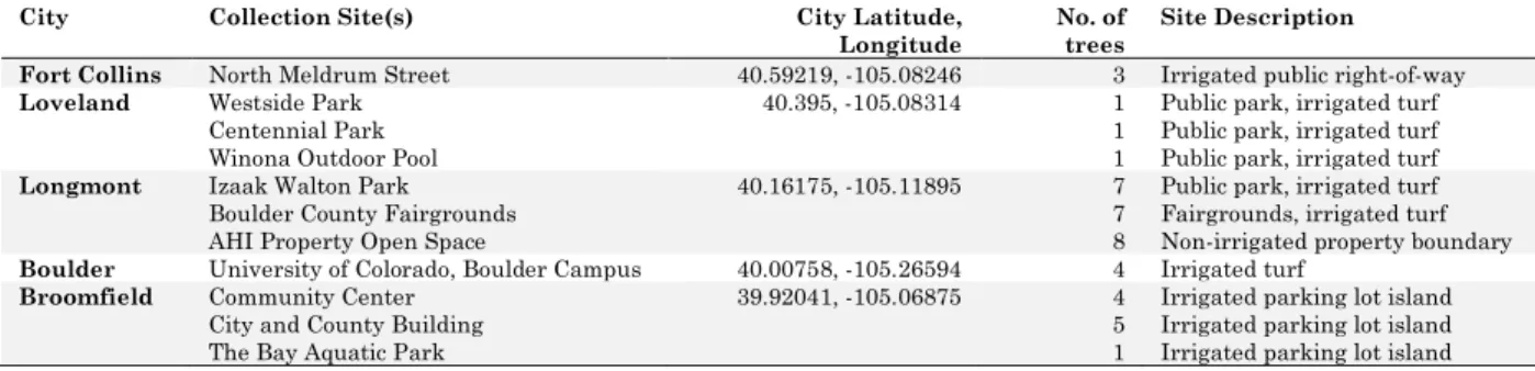
by Olson (2017) along with their origins. ... 12 Figure 3-1 Bland-Altman plots comparing mean observed green biomass versus published
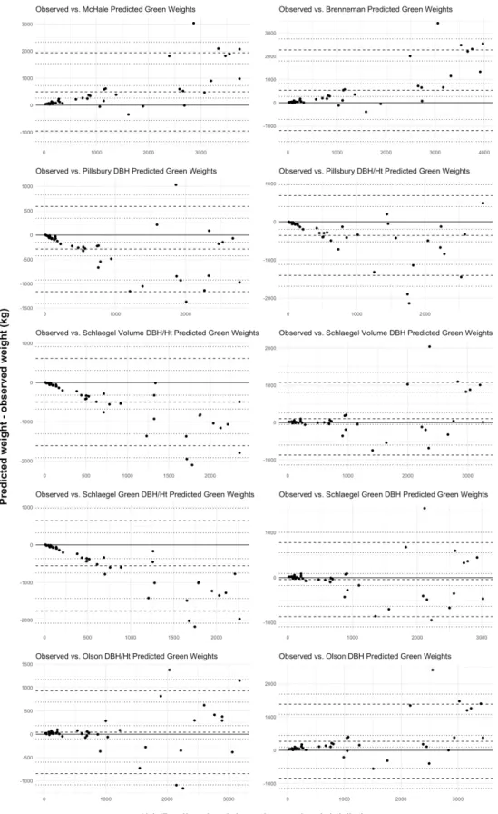
equation green predicted biomass. ... 38 Figure 3-2 Bland-Altman plots comparing mean observed oven-dry biomass versus
published equation oven-dry predicted biomass. ... 41 Figure 3-3 Plotted regression lines for locally-derived Northern Front Range green and oven dry biomass equations. ... 43 Figure 5-1 Scatterplots for observed green biomass and predicted biomass from green basis
equations for the 42 destructively sampled trees. ... 76 Figure 5-2 Scatterplots for observed oven-dry biomass and predicted biomass from oven-dry basis equations for the 42 destructively sampled trees. ... 77 Figure 6-1 Box and whisker plots representing the distribution of the residuals for green
basis published equations. ... 79 Figure 6-2 Box and whisker plots representing the distribution of the residuals for green
1. INTRODUCTION
Since its discovery in Detroit, MI in 2002, the emerald ash borer (EAB) (Agrilus
planipennis Fairmaire) has caused the death of hundreds of millions of ash trees (Fraxinus
spp.) in the U.S. and is considered to be the most destructive and costly invasive forest pest in U.S. history (Herms and McCullough, 2012). Sydnor et al. (2009) estimate that treating or removing 50% of the ash trees in urban areas in the U.S. will cost approximately $10.5 billion by 2019. This number does not include suburban areas, which are also often heavily planted with ash. Another important cost to municipalities and landowners is wood
disposal. Trees that are either killed by EAB outright or are preemptively removed are often chipped into mulch or disposed of in regulated landfill sites inside federal quarantine areas. The resulting volume of mulch from routine forestry operations, let alone mulch produced during peak EAB infestation, is often more than can be utilized by a municipality, and cities often pay to have mulch hauled away at considerable expense (Tom Wells and Kathleen Alexander, pers. comm.). Trees killed by EAB have generated an unprecedented amount of wood waste in states where the insect has become established, resulting in storage and disposal issues for those cities.
At the time of writing, Colorado is the westernmost state in which EAB has been detected, having been discovered in Boulder in September of 2013. Ash has been widely planted in many of Colorado’s communities due to its suitability as a street tree and its adaptability and ability to cope with Colorado’s changeable climatic conditions. Green ash is the most widely planted street tree in the Denver Metro Area of the Northern Front Range, and many Colorado communities’ urban forests are comprised of 15-20% ash on a per-stem basis, with percentages in individual neighborhoods of up to 70-80%. According to
Resource Group in Fort Collins, CO, ash trees constitute 33% of the city’s canopy cover (Ralph Zentz, pers. comm.), suggesting that ash contribute even more to the urban canopy than previously thought (a 2013 canopy assessment of the Denver Metro Area estimated ash populations on a per-stem basis), especially in cities that have many older, large diameter ash trees.
The cost of EAB management in the Denver Metro Area could be devastating to many cities’ budgets and will overwhelm forestry operations. The City of Denver has
estimated removal costs of $432 million (Wood, 2014). Additional economic losses associated with lost environmental services provided by the ash canopy in the Denver Metro Area, such as property value increases, stormwater mitigation, and air temperature reductions, could be as high as $82 million (Colorado State Forest Service, 2015; McPherson et al., 2013). Experience from other states managing EAB infestations has shown that the best way to avoid this is prior planning for the arrival of EAB by creating a comprehensive management plan that includes treatments to slow tree mortality so a controlled removal schedule can be implemented. Even with treatments, removals can quickly become unmanageable once EAB populations peak in an area, which has been estimated to occur around eight years after the initial arrival of the insect. Boulder is already experiencing this phenomenon in most areas throughout the city. Once this point is reached, wood volumes can become overwhelming as most cities do not have large sort yards able to handle the rate at which trees must be removed during peak infestations.
The Colorado Department of Agriculture’s Emerald Ash Borer Response Team has stated that comprehensive management plans including a wood utilization plan should be in place before the arrival of the insect (Colorado Department of Agriculture, 2014). The first step to understanding the potential impact of EAB in a community is a complete inventory of ash trees. Most cities do not include privately owned trees in municipal
inventories, but urban foresters have long used rule-of-thumb of 10:1 private to public trees. Inventories including routine measurements such as tree height and diameter at breast height (DBH, 1.37m) can be used to estimate biomass and give resource managers a better understanding of the amount of ash material produced from EAB-killed and
preemptively removed trees. McHale et al. (2009) produced biomass equations for 10
commonly planted tree species in the Fort Collins area, including green ash; however, these equations used LiDAR measurements to predict tree volume, and estimates were not
verified using harvested trees due to the difficulty in destructively sampling and weighing trees.
There are several real and perceived barriers to the utilization of urban wood, including logistical (transportation, lack of sort yards), financial (economics of processing urban logs for solid sawn timber products), unknown resource quantity (lack of complete inventories, and lack of knowledge of number of trees on private property), and marketing (perception of urban wood as low-value and lack of existing supply chain networks and markets). Some states have created successful urban wood utilization programs even prior to the arrival of EAB (Bratkovich, 2001), and several books and other resources that promote the utilization of wood from urban areas exist to help promote putting trees removed from urban forests to their highest value use rather than simply mulching the material or directing it to landfills (Brashaw et al., 2012; Solid Waste Association of North America, 2002).
To overcome these issues, more needs to be known about the quantity and quality of the ash resource across urban landscapes. While biomass equations exist for ash trees, they have often been developed for traditional forestry settings, and do not address the
Furthermore, the accuracy of biomass equations has been shown to be location specific (Pillsbury et al., 1998).
This thesis provides urban forest managers in Colorado’s Northern Front Range with a way to predict the amount of ash wood produced from trees preemptively removed as part of an EAB management strategy or from trees that are removed as they become
infested with EAB. This was achieved by developing an equation to accurately predict aboveground woody biomass for green ash trees growing in Northern Colorado’s urban forests. It is the intention that the equation will be incorporated into the Colorado Tree Coalition’s inventory and EAB cost calculator tool, CO-TreeView (https://cotreeview.com, n.d.). Municipal forest managers will have the ability to identify ash trees scheduled for removal from inventory data. The EAB tool will calculate a biomass quantity that can be used in debris disposal estimates. A specific gravity and moisture content value for this area is also of interest as these can further assist urban foresters, researchers and others interested in making accurate biomass estimations.
The objectives of this study were to determine: 1) whether locally developed, species-specific biomass equations outperform equations developed for areas outside of Colorado’s Northern Front Range; 2) the best predictive equation for above-ground woody biomass of green ash trees for emerald ash borer management activities in urban areas of Colorado’s Northern Front Range; and 3) whether the average wood specific gravity and moisture content of urban ash trees along Colorado’s Northern Front Range differed from published values.
These findings will assist urban forest managers in Colorado’s Northern Front Range in making management decisions regarding ash trees in response to the recent discovery of emerald ash borer in Colorado. Data and tools generated from this study can be
used in conjunction with municipal tree inventories to predict the amount of wood waste from EAB-killed trees in Northern Front Range urban areas.
2. LITERATURE REVIEW
2.1 Emerald ash borer and the issue of wood disposal
The emerald ash borer (Agrilus planipennis Fairmaire, EAB) presents an
unprecedented management challenge to urban foresters and other resource managers in the municipalities in which it has become established. Ash trees in the U.S. have no natural resistance to this pest, and EAB has no effective natural enemies outside of its native range. Mortality rates exceeded 99% for untreated trees 8 years after its detection at the original infestation epicenter in Michigan (Herms and McCullough, 2014). While effective treatments exist, not every ash tree is a good candidate for treatment because insecticides used to control EAB are systemic, therefore requiring that the tree’s vasculature is
uncompromised by previous injuries. Such pre-existing injuries (resulting from abiotic and biotic issues) are commonly found in ash trees in urban areas (Cranshaw, 2017; Jesse et al., 2011).
This invasive insect has been difficult to detect in Colorado since many of the symptoms produced by EAB-infested trees are also caused by Colorado’s often harsh climactic conditions, such as drought, unseasonable snowstorms and freezes, and other insect and disease problems. Many municipalities and other organizations managing ash trees have moved away from detection activities and instead are primarily focused on management activities, including conducting ash inventories, initiating treatment, and preemptive removal of ash trees with small diameter, trees in poor health, or trees in
undesirable planting locations. To date, Colorado communities have removed over 5,000 ash trees as the result of EAB management activities (Keith Wood, pers. comm.).
All too often the issue of wood disposal resulting from large numbers of trees killed by EAB is a low priority until the problem is present and the need to find solutions becomes
urgent. Many resources exist to aid municipalities in planning for the logistics of wood disposal (e.g., the Ash Utilization Options Project developed by the Southeast Michigan Resource Conservation and Development Council, Southeast Michigan RC&D, 2007), but the costs associated with disposal are not well documented. Several estimates for costs resulting from EAB infestations are available in the literature, but none specifically address wood disposal (Table 2-1 ). The insect has now spread to over 30 states and has killed hundreds of millions of ash trees. A means of predicting the amount of ash wood waste for budgetary and utilization purposes is therefore of great need and value to urban forest managers.
2.2 Biomass equations: Their uses and challenges
Allometric equations in forestry relate measurements of one or more tree
characteristics to another. In this way, an easy-to-measure characteristic, such as diameter at breast height, can be used to estimate whole tree volume or the volume of tree
components. Biomass estimates can then be extrapolated to different spatial scales (e.g., locally, regionally, nationally or continental) with volume-to-mass conversions using a species-specific wood density value (Asner et al., 2009; Chave et al., 2014; Dubayah et al., 2010; Pan et al., 2011). Equation development entails sampling the population of one or more species of interest and developing an equation representative of the entire population (Brand and Smith, 1985). Destructive sampling and weighing of whole trees is preferred since this is a direct measurement, but this method is often cost- and labor-prohibitive (Ketterings et al., 2001). Tree biomass equations were traditionally used for commercial forest management purposes, such as estimating the amount of merchantable timber in forest stands (e.g. Schlaegel, 1984), estimating the impacts of various forest management activities (e.g., Sollins and Anderson, 1971), to better understand nutrient cycling and other
bioenergy applications (e.g., Milbrandt, 2005). Biomass estimates are increasingly used for urban forest valuation and in carbon accounting to support climate change initiatives. The latter has resulted in numerous studies of forest structure and function, primarily in tropical areas (e.g. Banin et al., 2012; Chave et al., 2014; Chave et al., 2005; Chave et al., 2004; Ngomanda, 2014), but also Canada (Pasher et al., 2014), China (Fang et al., 2001), and other places. The U.S. Forest Service Forest Inventory and Analysis (FIA) Program provides comprehensive inventory data on U.S. forests. These data have been used for numerous analyses relating to forest structure and function including carbon accounting in U.S. forests (Brown, 2002; Houghton, 2005), and in worldwide carbon stock estimates (Pan et al., 2011), land cover and land use change (Homer et al., 2015; Lawler, 2014; McGarigal et al. 1995), the effects of disturbance (Asner et al., 2016, Cohen et al., 2016, Kurz et al. 2008), and developing biomass equations (Jenkins et al., 2003; Chojnacky et al., 2014).
Similarly, biomass equations have been used to study urban tree ecosystem services in the United States and elsewhere (e.g. McPherson et al. 2016, Roy 2012, Nowak et al. 2013). Applications include using allometric equations to predict various attributes of tree growth to assist with urban planning and management functions (for example, planning tree placement to avoid conflicts with structures and utilities based on estimated mature crown spread) (Peper et al. 2014, Pretzsch et al. 2015, Dahlhausen et al. 2016), and improving risk assessment related to tree failure by predicting biometric variables (Rust 2014).
Though there have been many studies related to allometry and biomass estimation, there are still many sources of uncertainty in developing accurate predictive equations. The challenges associated with the development and use of biomass equations are outlined subsequently.
Table 2-1 Summary of literature sources that provide tree removal costs related to EAB infestation.
Literature source Management activity Source of estimate Estimated cost Disposal costs1 Study area Hauer and Peterson
2017 Tree and stump removal Survey of 1723 communities in 50 US states Tree and stump removal costs increased from 20% of total urban forestry budgets prior to EAB infestation to 38.1% after infestation
N/A Survey of 1723 US communities
Kovacs et al. 2011 Tree removal and replacement Kovacs 2010 $800/tree residential and
non-residential; $600 parks N/A Twin Cities Metropolitan Area, MN Kovacs et al. 2010 Tree removal Purdue EAB Cost Calculator $850 - $2400/tree homeowner2
$150 - $1200/tree public N/A 25-state region centered on Detroit, MI McCullough and
Mercader 2012 Tree removal and replacement 2010 cost estimates from arborists or urban foresters in six Midwestern cities
$888 ± 54/tree Included in removal/replacement estimate
Simulated environment/ Midwestern US McKenney et al. 2012 Community overhead costs
(also includes managing the response, communication and monitoring activities)
City foresters in study area CAD $0.40/year for the duration
of an outbreak (USD $0.42) Included in community overhead costs 641 urban areas (pop. ≥ 1000) in eastern and western Canada
McKenney and Pedlar
2012 Tree removal City foresters and tree removal companies in study area CAD $16 - $20/cm DBH
3
(USD $16.78 - $20.97) N/A Canada Sadof 2017 Tree removal and stump
grinding City of Indianapolis, IN 2014 $14.00 - $36.00/cm DBH
4 N/A Indianapolis, IN
Sydnor et al. 2011 Tree removal – stump removal dep. on site: street and private yes, park no
Based on survey responses of
commercial arborists $413/tree private or street $331/tree park N/A Four-state area, including IL, IN, MI, WI Sydnor et al. 2007 Tree removal (stump removal
dep. on site: street and private yes, park no)
Based on survey responses of
commercial arborists $675/tree private or street $600/tree park N/A State of Ohio VanNatta 2012 Tree removal Based on MacPherson 2005,
which includes removal and disposal
$10/in DBH Included in removal
estimate University of Wisconsin, Stevens Point campus EAB Cost calculators
Hauer 2012 EAB Planning Simulator (EAB-PLANS)
Tree removal User specified User specified Does not include
functionality to specify wood waste disposal
Sadof 2016
EAB Cost Calculator Tree removal User specified User specified Does not include functionality to specify wood waste disposal
Model assumptions validated using EAB experience from cities in Indiana
1 A value of N/A indicates disposal costs were not specified, so it is unclear whether they are included in the cost of removal and/or replacement. 2 Estimates for trees 2.5 cm to >61 cm DBH.
3 Estimates for trees <20 cm to >40 cm DBH. 4 Estimates for trees 3 to >91 cm DBH.
2.3 The ambiguous origins of biomass equations
A large body of literature exists for development and use of tree allometric and biomass equations. Most U.S.-derived information for calculating wood volume and biomass relies on literature-based volume tables and specific gravity measurements developed decades ago, primarily for forests in eastern or Midwestern states (e.g., the publication by Clark et al. (1985) for the Gulf and Atlantic coastal plains is the green ash reference used by Jenkins et al., 2003, which is in turn used by the FIA Program for green ash across the U.S.). Newer references for wood characteristics simply aggregate a wide array of published values and report them in a compendium (e.g., Alden, 1995; Miles and Smith, 2009).
Likewise, biomass and volume equations may also be aggregated for a single or for multiple species (e.g., Ter-Mikaelian and Korzukhin, 1997), leaving the practitioner unsure which to use for a given purpose.
More place-based research is needed to support studies of climate change impact and worsening disturbances causing widespread tree mortality. Many newer studies are forced to rely on unsuitable equations due to the lack of more appropriate alternatives (McPherson et al., 2005). Uncertainty around the origin of equations, including the conditions under which they were developed, can lead to unintentional misuse of the equations and the opportunity for error propagation through time. Figure 2-1 and Figure 2-2 illustrate the origin of the equations used in the current study.
2.3.1 Sources of uncertainty and error in biomass equation development
The process of creating biomass and allometric equations unavoidably includes many sources of error. The main sources of error are sampling design, measurements in the field, and model development. The uncertainties associated with each are compounded throughout the biomass equation development process. Individual biomass studies often have limited sampling areas due to the challenging logistics required to sample even a
Figure 2-2 Biomass equations used to estimate green ash (F. pennsylvanica) and assessed by Olson (2017) along with their origins.
small number of trees, and it is questionable whether samples used in many biomass studies are truly random (Chave et al., 2004; Clark and Kellner, 2012; Paul et al., 2016; Temesgen et al., 2015). Samples may represent individuals taken from a single stand, or a small number of stands, or from an area that is easily accessible. In some cases, trees are weighed opportunistically when they are removed for reasons other than for research purposes (Lopez-Lopez, 2017; Olson, 2017). Trees of varying sizes, ages, and conditions are rarely represented in a single sample (McPherson et al., 2016). Small and large trees are often underrepresented (Chave et al., 2014), and there are idiosyncrasies associated with each: the amount of variance increases with tree size, and small trees are often inaccurately estimated with biomass equations because tree form changes during ontogeny (MacFarlane, 2015; Troxel et al., 2013). To provide an accurate representation of “average” trees, some datasets include only trees with full healthy crowns, leaving trees with less-than-perfect crowns underrepresented (Paul et al., 2016). These factors create uncertainty in model parameters (Temesgen et al., 2015).
There is no standard protocol for obtaining field measurements of destructively sampled trees (Weiskittel et al., 2015). Different weighing instruments are used, each having varying accuracy. Trees may be weighed using hanging scales, ground scales, or whole trees may be placed in a truck which is driven over a truck scale. Similarly, height measurements may be taken with a plummet, clinometer, a Biltmore stick (sighting), or other methods. Sometimes methods differ within a single study (Blood et al., 2015; Pretzsch et al., 2015). There are measurement errors associated with laboratory techniques used to determine moisture content and specific gravity. In addition, moisture content and specific gravity values are commonly based on a small number of samples for practical reasons (Paul et al., 2017). This is problematic because moisture content and specific gravity values
greatly influence biomass estimation, and each varies throughout the tree (Mate, et al., 2014; Paul et al., 2016, Weimann and Williamson, 2012).
There is a tradeoff between simple model forms using easy-to-measure variables and including more measurements that may improve model performance. Height is often
considered an important characteristic to include in biomass predictive equations (Chave et al., 2005; Duncanson et al., 2015). However, there is more measurement error associated with height than with DBH (Chave, et al., 2004; Ducey, 2012). Error in height
measurements is introduced when personnel are unfamiliar with measuring equipment (Kim, 2016) or simply because measurements are not taken correctly (Arias-Rodil et al., 2017). The error associated with taking certain measurements can outweigh the predictive accuracy achieved by including them (Temesgen et al., 2015; Weiskittel et al., 2015).
Lastly, there is a considerable amount of error introduced when developing biomass estimation models. Chave et al. (2004) found the most important source of error in biomass estimation comes from model selection. A thorough exploration of the data should be
performed, and model diagnostics consulted rather than relying solely on mechanical model selection processes or model dredging (Sileshi, 2014). While these processes select the most parsimonious form of the model based on specified criteria, such as AIC, these processes rely on the correct form of the full model being included in the selection process to begin with.
The combination of these sources of uncertainty can result in grossly erroneous biomass estimations. Sileshi (2014), Temesgen et al. (2015), and Weiskittel et al. (2015) provide comprehensive summaries of error propagation in biomass equation development.
2.3.2 Local, regional and species-specific equations
Many datasets used to develop biomass equations from harvested trees represent few individuals of a single species or a limited number of species. It is widely recognized
that species-specific, locally developed equations provide the most accurate biomass estimates (Basuki et al., 2009; Ngomanda et al., 2014).
Oftentimes, bias occurs when published equations are applied to areas outside of those for which they were developed. Timilsina et al. (2017) found the widely used i-Tree Eco model (i-Tree Eco v6.0, www.itreetools.org) developed by the U.S. Forest Service, and based on trees sampled in Chicago, Illinois by Nowak (1996), overpredicted leaf area of trees in Stevens Point, Wisconsin by 106%‒115%. Similarly, Boukili et al. (2017) found that the i-Tree Streets model and the newer U.S. Urban Tree Database (UTD) (McPherson et al., 2016) equations overpredicted carbon sequestration estimates in Cambridge,
Massachusetts when compared to empirical measurements combined with the UTD equations. McHale et al. (2009) found that the predictive capability of the published
equations they evaluated was inconsistent, and that depending on the equation source and the species to which the equation was applied, published equations underpredicted biomass by up to 76% and overpredicted by as much as 205%. The authors stated that some of the equations had been applied to trees outside of the diameter range for which they were developed, demonstrating that predictive equations become unreliable when applied to trees outside of the ranges for which they were developed (McHale et al., 2009).
There is evidence that biomass equations are highly location specific and it may not be appropriate to apply the same model across areas that aren’t relatively close in
proximity or similar in character to those for which they were developed. Escobedo et al. (2012) found that trees sampled in two subtropical forests in Florida yielded different carbon storage estimates. Pillsbury et al. (1998) found that no one predictive equation developed for each of seven sites across the range of a single species (Lithocarpus
examples demonstrate the need to use caution even when applying intraspecific equations to relatively small geographic areas.
2.3.3 Generalized, mixed species equations
Destructively sampling trees and developing species-specific, local equations is time consuming, labor intensive, and in many cases infeasible, especially if the trees to be measured must represent the average tree form (i.e., healthy trees with full crowns). General equations have been proposed by researchers attempting to balance accuracy of biomass estimates with the need to obtain suitable estimates within operational
constraints. Now that more datasets are publicly available, researchers have avoided the issue of small sample sizes by fitting new equations to multiple datasets. In this way, many individual trees representing one species are used to expand the size range and area
represented by the equations.
Jenkins et al. (2003) developed a series of 10 national-scale regression equations intended to provide consistent biomass predictions for all tree species found in the U.S. Jenkins et al. (2003) used a “modified meta-analysis” method after Pastor et al. (1984), which uses predictions (referred to as “pseudodata” by Pastor and others) from all discoverable published equations to refit new regression equations. Jenkins et al. (2003) grouped species according to taxonomic relatedness and similarities in specific gravity, then fit equations for each of these groups. Based on these groupings, green ash was placed in a general “mixed hardwood” category representing 289 data points from trees of 13 genera and over 20 species. This grouping contained plants ranging in form from small, multi-stemmed ornamental trees to large-maturing shade trees. Specific gravity values within this grouping ranged from 0.32 to 0.64. Pseudodata generated from 40 published equations were used to create new regression coefficients relating biomass to diameter at breast height. To extend the accuracy of the Jenkins et al. (2003) equations, Chojnacky et al.
(2014) provided a set of updated generalized biomass equations using refined taxonomical groupings that attempted to place individuals within family groupings. The authors further subdivided family groupings with wide ranges in specific gravity.
Generalized, mixed-species equations were not necessarily intended to replace species-specific biomass equations for smaller-scale biomass estimation; however, MacFarlane (2015) found generalized multi-species models based on an individual
components method applied at the stand level produced estimates that were as good as, or better than, species-specific models due to intraspecific variability in tree form at a local level, especially when a small number of trees are included in a sample. Paul et al. (2016) found generalized multi-species biomass equations created for Australian forests
representing a wide range of ecotypes predicted stand-level biomass with an accuracy of 99%.
In contrast, subsequent studies found that wide-scale generalized biomass equations produced biased estimates when applied at a finer scale. Zhou and Hemstrom (2009) used the Jenkins et al. (2003) equations to provide regional estimates of major softwood species in Oregon. This resulted in overpredictions of aboveground biomass by 17%. According to Zhou and Hemstrom (2009), local and regional equations are more appropriate when the goal is to obtain accurate biomass predictions at smaller scales in forests dominated by a few species. The authors recommended against using generalized wide-scale biomass equations without understanding the implications of doing so.
The national-scale models may produce biased biomass estimates even at the scale for which they were intended. A recent study by Domke et al. (2012) found that the Jenkins et al. (2003) national-scale biomass equations overpredicted biomass, and thus carbon, on a national scale when compared to the newer components ratio method (CRM; Heath et al.,
compared biomass estimates between the two methods for 20 of the most common tree species in the U.S. and found that the CRM provided estimates of national-scale biomass that were 16% lower than those produced using the Jenkins et al. (2003) approach.
Ironically, the authors attribute this reduction in estimated biomass to adding tree height into equations as a measurement variable. Jenkins et al. (2003) decided to exclude all equations that used height as variable in favor of DBH-only equations so they would be more accessible for practitioners.
Other studies have found that wide-scale generalized equations can perform accurately. Fayolle et al. (2013) found pan-tropical moist forest generalized multi-species equations developed by Chave et al. (2005) produced accurate predictions when applied to regions in central Africa, illustrating the range to which generalized equations may be extended. Fayolle et al. (2013) point out the importance of this finding given the magnitude of forestland requiring biomass estimation in central Africa and the absence of local
equations. Thus, generalized equations have a place where local equation development is not feasible due to limitations of resource availability, scale, or timeframe in which estimations must be done. However, these equations should be used with caution when accurate estimations of biomass are critical since it would be necessary to carry out national-scale mensuration campaigns to truly know the extent of bias associated with wide-scale mixed-species equations (Jenkins et al., 2003).
2.3.4 Other methods of indirect tree biomass measurement Allometric scaling theory
To create the most accurate predictive biomass equations, trees must be destructively sampled; that is, they must be cut down, meticulously measured, and weighed. The labor and cost involved in this endeavor commonly leads researchers to pursue non-destructive sampling methods acknowledged as less accurate, but more
practicable (Ketterings et al. 2001, Pearson et al. 2007, McHale et al. 2009, Ngomanda et al. 2014). Equations based on various allometric scaling theories, first described by Huxley and Tessier (1936), have led to several attempts to create an idealistic representation of tree form, invariant across species, environment, age or location, thus eliminating the need to destructively sample trees (Pilli et al., 2006). These include Metabolic Scaling Theory (MST), and the Geometric Similarity and Stress Similarity models. Each theory attempts to explain archetypical growth based on physical constraints, such as the tree’s ability to effectively transport water throughout, or mechanically support the entire organism (Enquist, et al., 2009; West, 1999).
Attempts by subsequent studies to substantiate these models have shown that tree form does not follow universal scaling rules when architecture is affected by environmental conditions (Feldpausch et al., 2011; Lines et al., 2012; Lopez-Serrano et al., 2005; Motallebi and Kangur, 2016), competition (Forrester et al., 2017; Poorter et al., 2003), disturbance (Moncrieff et al., 2011; Tredennick et al., 2013), or in cases where a tree’s canopy is altered by management activities such as pruning (Peper et al., 2001; Rust, 2014). By definition, allometry relies upon stable scaling relationships; therefore, scaling laws do not adequately describe trees whose forms are altered by adverse growing conditions, pruning, insect damage, or mechanical damage.
Remote sensing of biomass
Remote sensing techniques are increasingly used to create biomass estimates. Terrestrial laser scanning has been used to produce biomass estimates of individual trees in lieu of costly destructive sampling techniques (McHale et al., 2009; Lefsky and McHale, 2008; Stovall et al., 2017). Larger scale estimation is accomplished via airborne LiDAR scanning or satellite imagery (Lefsky et al., 2005; Muukkonen, 2007; Ploton et al., 2012).
diameter tapes are still more accurate than remote sensing methods (Dassot et al., 2010; Dittmann et al., 2017; Weaver et al., 2015; West, 2009) because errors in sampling, measurement, and model selection are combined with errors associated with the remote sensing equipment used (Clark and Kellner, 2012). For instance, Vastaranta et al. (2009) found laser-based measurements of height and DBH varied widely depending on the equipment used. However, the authors determined that errors for some methods were within “acceptable limits” given traditional measurement instruments (such as calipers in the case of DBH) had similar error rates.
Remote sensing is prone to the same sources of error as biomass indirectly estimated with allometric techniques because direct measurements needed to calibrate these methods are also error-prone. Further, there are additional sources of error inherent to remote sensing equipment. While remote sensing may not produce estimates as accurate as other indirect allometric techniques or destructive sampling, the technology is evolving quickly, and these methods have the advantage of being able to achieve biomass estimates over large areas that are otherwise impractical, and in a short amount of time without the need for removing and weighing trees (Stovall et al., 2017).
2.4 The lack of urban, species-specific biomass equations
The problem of scale and unrepresentative datasets is compounded in the case of urban-based biomass equations. This is a comparatively new area of interest with relatively few extant urban-specific studies. This paucity underscores the need for urban-based
equations, since there are many well-documented differences between open-grown trees and those grown in natural forests (McPherson and Peper, 2012; McPherson et al., 2016; Zhou et al. 2015).
Urban trees are often open-grown and intensively managed. Management regimes with different pruning, supplemental irrigation and fertilization, and tree placement
approaches result in trees with architecture varying widely from one location to another and differing from the “average” form of a forest conspecific (McHale et al., 2009; McHale and Lefsky, 2008; McPherson et al., 2016, Peper et al., 2014; Quigley, 2004). Though there is an amount of genetic control exerted over tree form, tree growth habit, and thus biomass allocation, are plastic and are strongly influenced by growing conditions (MacFarlane, 2015; Pretzsch and Dieler, 2012). Urban trees are often not native to the area—and thus
climate—in which they are planted. This, along with a host of various anthropogenic stressors found in urban environments such as compacted soils, planting sites that offer limited rooting space, impervious surfaces leading to increased temperatures and reduced soil water, pollutants and contaminants, and insufficient irrigation, all influence tree growth, often in the form of a decrease (Jim, 1998; Quigley, 2004). Each of these factors can produce differences in growth within and across sites (Blood et al., 2016; McPherson and Peper, 2012).
As noted in section 2.2.1 (Figure 2-1 and Figure 2-2), it is often difficult to determine the provenance of published equations. Equations used for urban areas are typically based on those developed for natural forests in areas with different growing conditions from the locations in which the equations are applied. When an equation is used in an urban study it is often reused by subsequent urban studies, and the original source of the now “urban” equation becomes unclear. Authors self-cite, further obfuscating the origin of an equation (e.g., Nowak et al., 2013). Equations used for green ash are often equations developed for other species of ash (Brenneman, 1978; Bunce, 1968; Pillsbury et al., 1998), or are
generalized equations applied to a large group of related or unrelated species (Jenkins et al., 2003; Chojnacky et al., 2014). Unintended misuse of forest-derived equations occurs when forest equations are applied to urban areas without understanding their provenance.
If an equation is cited in an “urban” study, this equation is often reused in studies in other urban areas, resulting in error propagation over time.
To account for differences between urban trees and those growing in forested areas, published correction factors have been proposed and are intended to be used in conjunction with forest-derived equations for open grown trees. One such correction factor from a study by Nowak (1994) found forest-derived equations overpredicted urban tree biomass by 20%. Nowak (1994) proposed that biomass estimates from forest-derived equations be multiplied by 0.80 in all urban areas to reflect this difference. This correction has often been used without regard to the potential differences in tree biomass based on factors such as regional climactic, site, and management differences mentioned previously (e.g., McPherson, 1998; Nowak and Crane, 2001; Nowak et al., 2008; Strohbach and Haase, 2012; Yang et al., 2005; Zhao et al., 2010). A different correction suggested by Zhou et al. (2011) states that biomass estimations for open-grown trees be multiplied by a correction factor of 1.2. This 20%
upward correction in biomass directly contradicts Nowak’s suggested use of a 20% decrease. While the trees in both cases are pruned and grown in open conditions, the difference
highlights that such corrections cannot be applied generally or without scrutiny and reinforces the need for a greater understanding of factors contributing to variations in urban tree growth across locations.
In an attempt to address these matters, the U.S. Forest Service Pacific Southwest Research Station recently introduced their Urban Tree Database and Allometric Equations (McPherson et al., 2016). Though this resource provides numerous equations for the most widely grown tree species in the 17 cities covered by the study, the authors stress the need to continue improving the accuracy of urban biomass equations by obtaining data for more regions across the country.
3. GREEN ASH (FRAXINUS PENNSYLVANICA MARSH.) BIOMASS EQUATIONS FOR URBAN TREES REMOVED IN RESPONSE TO THE EMERALD ASH BORER
(AGRILUS PLANIPENNIS FAIRMAIRE)
3.1 Introduction
Since the arrival of the emerald ash borer (Agrilus planipennis Fairmaire) in the United States in 2002 (Haack et al., 2002; Cappaert et al., 2005; Poland and McCullough, 2006), urban forest managers have been faced with an unprecedented challenge. Emerald ash borer (EAB), labeled as the most destructive forest pest in United States history (Herms and McCullough, 2014), has caused the death of hundreds of millions of ash trees (Fraxinus spp.) in the 34 U.S. states in which it has been detected. Since eradication of EAB is infeasible due to the difficulty of detection (Herms and McCullough, 2014; Knight et al., 2014; McCullough et al., 2009), most emerald ash borer management programs aim to slow the spread of the insect to give urban forest managers time to respond (Fahrner et al., 2017; McCullough and Mercader, 2012).
Costs for treating and removing trees is expected to reach USD $10.5 billion by the year 2019 (Sydnor et al., 2009). However, the cost estimates for EAB management activities presented by Sydnor et al. (2009), Kovacs et al. (2010; 2011), Hauer and Petersen (2017), Sadof et al. (2017) and others do not include wood disposal costs, or combine disposal costs with those for other management activities. Costs can be expensive at the local scale; for example, between March, 2015 and April, 2016, wood disposal costs for the City of Boulder’s Forestry Division related to EAB and a winter kill event primarily affecting Siberian elm (Ulmus pumila) trees were approximately USD $35,000 (Kathleen Alexander, pers. comm.).
municipal solid waste (EPA, 2016). Nash (2009, unpublished thesis) estimated that 128,292 tons of urban forest residues were generated in the Tri-City Area of the Northern Front Range annually, an area including the cities of Fort Collins, Loveland and Greeley. Of this, the study found that approximately 40 percent of the material was disposed of in landfills while the remaining fraction was taken to wood recycling facilities to be turned into mulch, compost, or firewood.
The Colorado State Forest Service developed a statewide inventory tool, CO-Tree View (https://cotreeview.com, n.d.), to assist Colorado municipalities in creating accurate ash tree inventories as the first step in creating an EAB management plan. The software includes an EAB cost calculator which currently allows urban forest managers to estimate planned treatment, removal, and replacement costs for ash trees. It does not include a way to predict costs of ash wood disposal. There is a need for an accurate method to predict and budget for wood disposal costs as part of a comprehensive emerald ash borer management plan (Colorado Emerald Ash Borer Response Team, 2015).
Part of the difficulty in making such predictions is that biomass equations are regionally specific. Environmental factors and site conditions affect tree growth, leading to intraspecific differences in allometric relationships, thereby decreasing prediction accuracy when equations are applied to areas for which they were not developed (Duncanson et al., 2015; Hulshof et al., 2015, Urban et al., 2010). For instance, Forrester, et al. (2017) and Hulshof et al. (2015) found that trees growing in cold, arid environments and whose climates experienced high seasonal variability were shorter than those growing in areas experiencing less extreme environmental conditions. These conditions are similar to those found along Colorado’s Northern Front Range.
In using existing forest and urban equations to predict biomass of urban green ash trees in Fort Collins, Colorado, McHale et al. (2009) found that biomass predictions from
these equations ranged from a 27% overprediction to a 96% underprediction of total
aboveground woody biomass woody biomass when compared to detailed tree measurements taken with ground-based LiDAR. Furthermore, Blood et al. (2016) found that models were location-specific, and that models developed for one location may not provide accurate predictions when applied to another location in the same climactic zone or region.
McPherson and Peper (2012) found that green ash growing in Cheyenne, Wyoming were consistently smaller than same-aged trees in nearby Fort Collins, Colorado, likely due to Cheyenne’s harsher climate and poorer soil conditions.
Current green ash aboveground woody biomass (AGB) predictive equations have largely been developed for areas in the eastern and Midwestern states, or Canada (e.g. Bunce, 1968; Peper et al., 2014; Schlaegel, 1984). Furthermore, most have been developed for trees growing in natural forests, not urban areas. Due to the unique and varied growing conditions of urban trees versus those growing in natural forests, and the climactic
differences between Colorado’s Front Range versus the Midwest and eastern United States, it is uncertain whether these equations provide adequate predictions of biomass for green ash growing in Colorado’s urban areas.
The study conducted in Fort Collins, Colorado by McHale et al. (2009) provided volume equations for ten urban street tree species, including green ash. Measurements of individual trees were obtained using ground-scanning LiDAR as part of a carbon storage analysis of urban trees in Fort Collins, Colorado. These equations were not validated using destructively sampled trees. Although removing and directly weighing trees remains the most accurate measure of tree biomass (McHale et al., 2009; Nelson et al., 1999; Nogueira et al., 2008), researchers commonly use non-destructive sampling methods to estimate biomass due to prohibitive cost and labor requirements.
Furthermore, specific gravity is another important attribute influencing mechanical and physical properties of wood, such as the quality of wood used for solid sawn products, paper and pulp, and wood energy applications (Shmulsky and Jones, 2011; Zobel and van Buijtenen, 1989). Specific gravity values may be converted to density values, which can then be used in volume-to-mass calculations whereby a known volume is multiplied by a known density to produce a mass. These calculations are widely used for estimating
biomass for individual trees as well as on varying spatial scales from single stands to entire landscapes. Specific gravity values for urban trees are largely absent from the literature (McHale et al., 2009). Values from sources such as Alden (1995) and Miles and Smith (2009) have long been the standard for green ash and other tree species in the United States, but as is the case with the aforementioned biomass equations, these measurements were
primarily taken from natural forests in areas whose climates differ greatly from Colorado’s. Specific gravity is influenced by climate, growing conditions, and management regimes (Whitmore 1973; Wiemann and Williamson 1989; Wiemann and Williamson 2007), and differs between forest-grown and open-grown trees (Zhou et al., 2011); therefore, published values may not accurately represent wood specific gravity of green ash trees growing in Colorado’s Northern Front Range cities.
The objectives of this study were to determine: 1) whether locally developed, species-specific biomass equations outperform equations developed for areas outside of Colorado’s Northern Front Range; 2) the best predictive equation for above-ground woody biomass of green ash trees for emerald ash borer management activities in urban areas of Colorado’s Northern Front Range; and 3) whether the average wood specific gravity and moisture content of urban ash trees along Colorado’s Northern Front Range differed from published values. To accomplish the first objective, predictive accuracy of existing published
pairwise multiple comparisons with repeated measures. To accomplish the second objective, locally-derived equations for Colorado’s Northern Front Range were developed and
compared to existing biomass equations that have been used for urban green ash biomass prediction. Published specific gravity and moisture content values were compared to locally-derived values for Colorado’s Northern Front Range to accomplish the third objective. Identifying biomass equations and specific gravity and average moisture values suitable for green ash along Colorado’s Northern Front Range will allow resource managers engaged in EAB wood disposal efforts and urban forest mensuration initiatives to more accurately estimate green ash biomass.
3.2 Methods 3.2.1 Study area
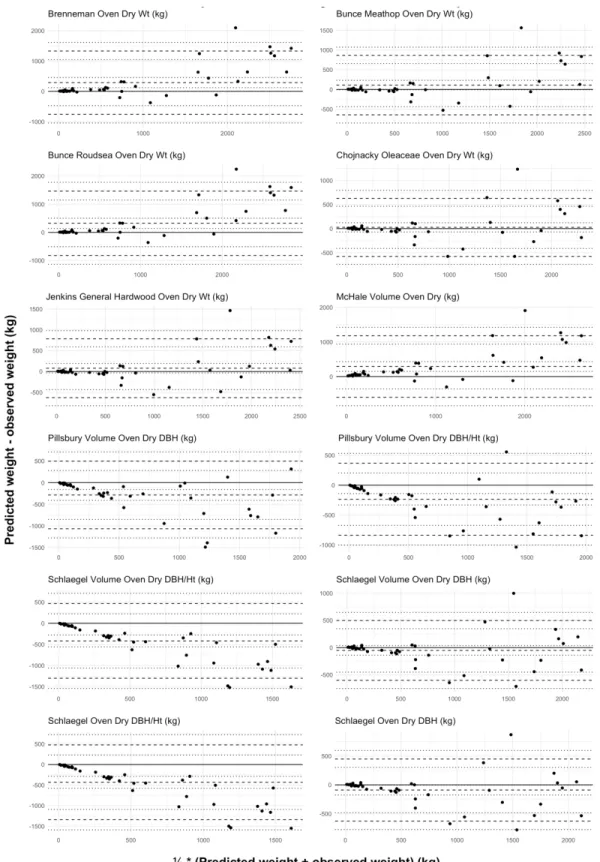
For this study, 42 green ash trees were destructively sampled at 11 sites in publicly-managed parks, rights-of-way, and municipal open spaces in five cities along Colorado’s Northern Front Range Urban Corridor (Chronic and Chronic, 1974): Fort Collins, Loveland, Longmont, Boulder and Broomfield. Location attributes can be found in Table 3-1.
Table 3-1 Northern Front Range cities from which green ash trees were destructively sampled during this study.
3.2.2 Field measurements
Trees were measured, removed, and weighed after leaf-drop during the early spring of 2016, and the fall of 2016 through the winter of 2017. Foliage biomass was not included
City Collection Site(s) City Latitude,
Longitude No. of trees Site Description
Fort Collins North Meldrum Street 40.59219, -105.08246 3 Irrigated public right-of-way
Loveland Westside Park
Centennial Park Winona Outdoor Pool
40.395, -105.08314 1 1 1
Public park, irrigated turf Public park, irrigated turf Public park, irrigated turf
Longmont Izaak Walton Park
Boulder County Fairgrounds AHI Property Open Space
40.16175, -105.11895 7 7 8
Public park, irrigated turf Fairgrounds, irrigated turf Non-irrigated property boundary
Boulder University of Colorado, Boulder Campus 40.00758, -105.26594 4 Irrigated turf
Broomfield Community Center
City and County Building The Bay Aquatic Park
39.92041, -105.06875 4 5 1
Irrigated parking lot island Irrigated parking lot island Irrigated parking lot island
given the goal of the study was to determine aboveground woody biomass (AGB) on both a green and oven-dry basis. The destructively sampled trees had been designated for removal prior to the study as part of planned efforts to reduce the number of ash trees at risk from EAB. Removal locations were in cities willing to provide trees, staff, and equipment required for destructive sampling.
Measurements included diameter at breast height (DBH) measured in cm at 1.3 m from the base of the tree, total tree height (m), and height to the first live branch (m). Percent canopy thinning was recorded using the ash canopy thinning scale created for emerald ash borer-infested ash trees in Michigan by Smitley et al. (2008). Additional data collected included whether or not the tree was infested with EAB as evidenced by the presence of larval feeding galleries or larvae, whether the tree was dead, and whether the tree was multi-stemmed (defined as having two or more leaders starting below diameter at breast height). Summary statistics for the trees sampled for this study are presented in Table 3-2.
Table 3-2 Summary statistics for trees destructively sampled for this study. Numbers in parentheses represent the standard deviation of each measurement.
Twigs and branches less than 10.16 cm (4 in) in diameter were processed in a chipper. Chips were blown directly into Flexible Intermediate Bulk Containers (FIBCs) attached to the spout of a drum-style wood chipper. Each FBIC was weighed on a low-profile floor scale (Uline model H-754, 2267.96 kg (5000 lb) x 0.453592 kg (1 lb)). The FBICs were of known weight, and the weight of the container was subtracted from each FBIC of chips weighed to obtain biomass of twigs and branches < 10.16 cm. A representative sample of chips per tree were collected from the FBICs at different points during the chipping
DBH (cm) Branching Ht. (m) Tree Ht. (m) % Crown Dieback Total Green Wt. (kg)
Range 7.6 - 66.0 0.63 - 6.40 2.79 - 20.12 0 - 100 7.26 - 3276.30
Mean 33.9 (8.5) 2.28 (1.11) 10.0 (4.03) 22.41 (31.53) 1051.25 (1028.27)
process for later laboratory processing to determine moisture content (MC). Each sample bag was given a unique identifier associating it with a specific tree. Larger woody material was broken down into two size classes, and each was weighed separately: branches 10.16 cm (4 in) in diameter up to 25.4 cm (10 in) in diameter, and logs 25.4 cm or greater in diameter. Branches and logs were weighed whole when feasible; if they were too large to rest on the scale they were sectioned, and the weight of the sections summed for a total branch or log biomass.
Wood cross sections were removed from the stump end of the main stem and top of one > 25.4 cm log of each tree to later be used in determining MC in the lab. Paul et al. (2017) demonstrated that, if it is not feasible for reasons of practicality to collect moisture samples from many locations throughout the tree, then collecting representative samples of the bole and crown to use in MC estimation best approximates whole-tree moisture.
Moisture loss was mitigated by wrapping tree cross sections in plastic as soon as they were cut. Once the cross sections were relocated to the laboratory at the end of each field day, the bags were placed in large plastic tubs with tight-fitting lids to further prevent moisture loss until the samples could be processed.
3.2.3 Laboratory measurements
Whenever possible, sample processing in the laboratory was completed the day following sample collection to minimize changes in MC from the time the tree was felled to the time green wood measurements were taken.
Wood moisture content and specific gravity
Each cross section was de-barked and sawn into portions. All cuts were made through the pith of the cross section to capture differences in specific gravity from the cambium to the pith (Wiemann and Williamson, 1989; Woodcock and Shier, 2002;
whether the portion was from a cross section from the top or the bottom of the main stem, and the tree from which it was cut. Each cross-section portion was then weighed to obtain its green weight (g). After each portion was weighed, it was placed into a tub of water for at least 48 hours to ensure the cell walls exceeded fiber saturation point (FSP). FSP is defined as the point at which free water has been removed from cell lumina, but the cell walls are saturated. Above FSP point, the dimension of the wood does not change as a function of moisture content (Glass and Zelinka, 2010).
As outlined in American Society for Testing and Materials Standard D2395 Method B, Mode II, once each cross-section portion reached FSP, its green volume was measured using water displacement. The weight in grams of the water displaced when the specimen was fully submerged was used to represent the specimen’s volume in cm3. Specific gravity was measured on a green basis (basic specific gravity) using the equation:
SGBasic = MOD / (VolGreen * ρwater)
where:
MOD is the oven-dry weight of wood in g VolGreen is the green volume of wood in cm3
ρwater is the density of an equal volume of water in g/cm3
After obtaining volume measurements, each cross-section portion was placed in an oven maintained at 105° C. Weight was checked periodically until it remained unchanged for at least three consecutive hours, at which time the portion was considered to have reached oven-dry status. Drying time ranged from 2 days for small samples to 4 days for large samples. Cross-section portions were then reweighed, and their weight recorded in grams. The moisture content as a percentage of the green weight of the cross-section pieces was calculated using the formula:
where:
MC% is the moisture content of the wood expressed as a percentage WG is the green weight of the chips or cross section pieces (g)
WOD is the oven-dry weight of the chips or cross section pieces (g)
Moisture content of chips
The green weight of a sample of chips taken from the FBICs representing twigs and small branch wood < 10.16 cm diameter for each tree were weighed (g). The chips were then placed in an oven at 105° C, and their weight was checked periodically until it remained unchanged for at least three consecutive hours, at which time the chip specimens were considered to have reached oven-dry status. Drying time took approximately 48 hours. The chips were then re-weighed and their weight recorded in grams. Moisture content of the chips was measured using the same method outlined previously for cross sections. The percent moisture content for the chips and two cross sections collected from each tree were used to obtain an estimate of the moisture content of the whole tree.
3.3 Statistical analysis
All statistical analyses were done using R Studio statistical software version 1.0.153 (R Studio Team, 2015). A significance level of ∝ = 0.05 was used for all statistical tests.
3.3.1 Evaluation of published green ash biomass equations
The Fort Collins, Colorado equation developed by McHale et al. (2009) and the equations identified as having been used in other urban biomass studies by McHale et al. (2009) were evaluated in this study (hereafter, the McHale equation). Some of the equations evaluated by McHale et al. (2009) had several forms (e.g. volume, oven-dry weight, green weight), and since it was not always clear which form of the equation was used, all forms of each literature equation evaluated by McHale et al. were included (hereafter, the
Brenneman equations, Bunce equations, Pillsbury equations, and Schlaegel equations). Another green ash biomass equation developed by Olson (2017) using destructively-sampled urban green ash in the Twin Cities Metro Area, Minnesota was evaluated (hereafter, the Olson equation), in addition to an equation developed by Jenkins et al. (2003) (hereafter, the Jenkins equation) since it was one of the underlying published equations assessed in that study.
An equation developed by Hahn (1984) evaluated in the Twin Cities study was not included in the comparisons of published green ash models for three reasons: 1) comparing models for which data collection methods were different introduces error into the
comparisons (Sileshi, 2014); 2) it is unlikely that urban forest managers would routinely take the measurements specified by Hahn as part of their tree inventory process (cull percentage, volume of a 1-foot stump, etc.); and 3) if total tree mass is the measurement of interest, as was the case in the present study, a total mass equation may perform better than a components-based equation (McFarlane, 2015).
Lastly, because Olson evaluated the performance of the national scale biomass equation developed by Jenkins et al. (2003), the updated national scale biomass equation developed by Chojnacky et al. (2014) (hereafter, the Chojnacky equation), was also evaluated. Chojnacky et al. (2014) used finer-scale groupings than in the Jenkins et al. (2003) equations to improve estimates. A list of the equations evaluated in this study can be found in Table 3-3.
One-factor repeated measures using linear mixed-effects models (Pinheiro and Bates 2000) allow for comparison of the mean predicted weight (biomass) of each equation for each tree. In this way, published equation predictions of biomass were compared to measured green and measured oven-dry biomass. This methodology is common in the
Table 3-3 Green ash biomass equations evaluated in this study. All are for total aboveground woody biomass minus foliage. Equation source Species1 Equation Quantity measured (Y) Moisture
basis2 a b c n DBH range (cm)
McHale et al., 2009 Green ash tvol = a(DBH)^b Volume (kg/m3) N/A 0.0005885 2.206 --- 15 14.8-122.6
Brenneman, 1978 White ash Y = a x^b Biomass (lbs)
Biomass (lbs) Oven-dry Green 4.1914 2.3626 2.4309 2.4798 --- --- 15 5.1-50.8 Bunce, 1968
Meathop Roudsea
European ash loge y = a + b (loge (DBH))
Biomass (kg)
Biomass (kg) Oven-dry Oven-dry -5.308133 -5.386958 2.488218 2.546645 --- --- 15
9.0-104.0 9.5-57.5 Pillsbury, 1998 Modesto ash V = a(DBH^b)
V = a(DBH^b)(Ht^c) Volume (lbs/ft
3)
Volume (lbs/ft3) N/A 0.022227 0.001287 2.633462 1.762964 1.427822 50 14.5-84.8
Schlaegel, 1984 Green ash ln(Y) = b0 + b1 ln(D^2*H) ln(Y) = b0 + b1 ln(D^2) Volume (lbs/ft3) Biomass (lbs) Biomass (lbs) Volume (lbs/ft3) Biomass (lbs) Biomass (lbs) N/A Green Oven-dry N/A Green Oven-dry -5.371 -1.104 -1.759 -2.644 1.518 0.935 0.92436 0.88814 0.91023 1.17048 1.12431 1.1515 --- --- --- --- --- --- 70 2.3-77.7 Olson, 2017 (Jenkins
refit) Green ash Bm = exp(b0 + b1 log(DBH)) Bm = exp(b0 + b1 log(DBH) + b2 log(ht)) Biomass (lbs) Biomass (lbs) Green Green 1.8865 0.4693 2.2166 1.8394 0.6316 --- 38 7.6-83.8 Jenkins et al., 2003 Mixed hardwood spp. Bm = exp(b0 + b1 ln DBH) Biomass (kg) Oven-dry -2.48 2.4835 --- 148 2.54-27.69 Chojnacky et al., 2014 Oleaceae spp., specific
gravity < 0.55 ln(biomass) = b0 + b1 ln(DBH) Biomass (kg) Oven-dry -2.0314 2.3524 --- Unk. 3-42
1Species for which the published equation was developed. 2Moisture basis as indicated by author.