The Impact of Human Capital
on Economic Growth:
Evidence from the European Economic Area
MASTER THESIS WITHIN: Economics NUMBER OF CREDITS: 30
PROGRAMME OF STUDY: Economic analysis AUTHOR: Marko Ilić
Master Thesis in Economics
Title: The impact of human capital on economic growth: Evidence from the EEA Author: Marko Ilić
Tutor: Andreas Stephan
Date: 2020-05-24
Key terms: Human Capital; Economic Growth; European Economic Area; Education
Abstract
The study examines whether human capital accumulation is related to the economic growth of the EEA countries. Several different human capital proxies are being deployed – secondary school enrolment of males, total tertiary school enrolment, average years of schooling, and total education expenditure. Moreover, the analysis has been carried out in the period from 1999-2019 and on 3 different levels concerning the structure of the sample- full EEA-31 sample, the sample consisting of the relatively high-income EEA countries, and the sample made of the relatively low-income EEA countries. The results indicate that a 1-year lagged value of education expenditure positively influences the economic growth within the full EEA sample. Additionally, when only higher-income EEA countries are taken into the analysis, secondary school enrolment of males, total tertiary school enrolment, and education expenditure all appear to have statistically positive effects on economic growth with the estimated coefficients of .001, .012, and .055. respectively. However, there have not been shreds of evidence of such effects of human capital on economic growth in the less developed countries of the EEA formation.
Contents
1.
Introduction ... 1
2.
Background of Economic Growth ... 4
2.1 Neoclassical Growth Theory ... 4
2.2 Endogenous Growth Theory ... 6
2.3 Human Capital and Economic Growth ... 7
3.
Theoretical Framework ... 11
4.
Methodology and Model ... 12
5.
Data Description ... 13
6.
Empirical Analysis and Discussion ... 17
6.1 Descriptive statistics and visualization ... 17
6.1.1 Education expenditure and economic growth ... 18
6.1.2 School enrolment and economic growth ... 20
6.1.3 Years of schooling and economic growth ... 22
6.2 Regression Analysis ... 23
6.2.1 Effects of education ... 26
6.2.2 Effects of Control Variables ... 27
6.3 The EEA countries segregation ... 29
6.4 Sensitivity check ... 32
7.
Conclusion ... 35
8.
Bibliography ... 37
Figures
Figure 1: Mean logged values of GDP per capita growth against mean values of education expenditure
... 20
Figure 2: : Mean logged values of GDP per capita growth plotted against mean values of male secondary school enrollment ... 21
Figure 3: Mean logged GDP per capita growth plotted against mean values of average years of schooling. ... 22
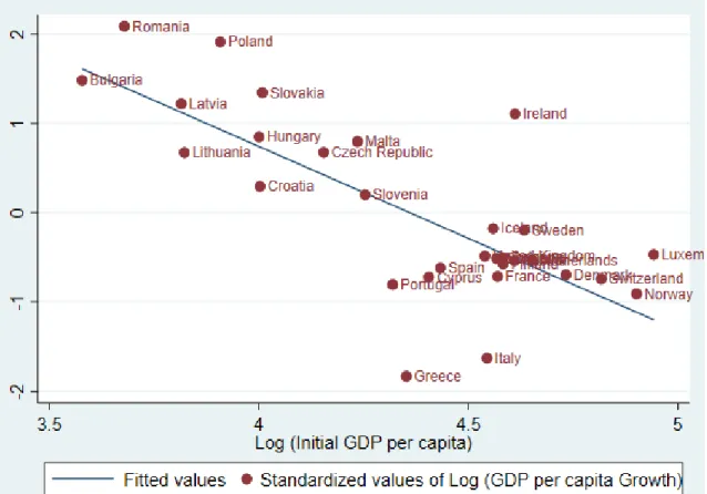
Figure 4: Mean logged values of GDP per capita growth plotted against initial values of GDP per capita in 1999. Source ... 28
Figure 5: Comparison between the EEA countries based on the average GDP per capita in the period from 1999-2019. ... 29
Tables
Table 1: Cross-study relationship between human capital and economic growth ... 10Table 2: Human Capital Measurement ... 15
Table 3: Description of Control Variables ... 16
Table 4: Descriptive statistics ... 17
Table 5: Growth rates of EEA countries and their education expenditures ... 18
Table 6: Hausman test ... 23
Table 7: Modified Wald test for groupwise heteroskedasticity ... 23
Table 8: Fixed-effect panel regression with robust estimators ... 24
Table 9: Education effects comparison between the 2 groups ... 30
Table 10: Fixed effect panel regression using a 1 year lagged value of education expenditure ... 33
Appendix
Table A 1: GDP per capita growth and tertiary school enrollment across the EEA countries in the period from 1999-2019 ... 39Table A 2: Correlation Matrix ... 41
Table A 3: Logged GDP per capita growth of all 31 EEA countries over the observed period ... 42
Table A 4: Levin-lin-chu unit root test for log (GDP per capita growth) ... 43
Table A 5: Wooldridge test for autocorrelation in panel data... 43
Table A 6: Multicollinearity test ... 44
Table A 7: GDP per capita of the EEA countries in 2019 ... 45
Table A 8: Upper and lower GDP per capita group ... 46
Table A 9 : Comparison between the groups ... 47
Figure A 1: Mean logged values of GDP per capita growth plotted against mean values of enrollment into tertiary education. 40 Figure A. 2: Logged GDP per capita growth of all 31 EEA countries over the observed period ... 41
Figure A. 3: Mean differences in average years of schooling and education expenditure between the groups. ... 46
1. Introduction
Globalization and international trade force countries and their economies to compete with each other in order to acquire and maintain a competitive advantage. To accomplish that aim, countries’ authorities are striving to identify the main factors of the growth of their economies. Investing solely in capital stock and fixed asset seems to be an outdated formula for economic growth which was mostly prevalent until the 19th century. Hence, it has been crucial to recognize the key prerequisites for economic progression.
One of the main factors that have gained enormous attention over the past decades is human capital accumulation. Human capital represents an intangible asset and can be defined as the economic value of a worker’s experience and skills which are mainly acquired through education and training. The importance of human capital accumulation has roots in a belief that a country’s economy tends to be more productive as the portion of educated workers increases since more educated workers are capable of carrying out complex tasks that require literacy and critical thinking (Radcliffe 2020)
Countries with a greater portion of the educated population see faster economic growth in comparison to countries with less-educated workers (Temple 1999). It implies that those two phenomena, economic growth, and increase in human accumulation, have been moving in the same direction in recent time. In other words, they seem to be positively correlated.
Thus, it seems logical that governments, especially in the more developed countries, are investing more than ever before in educating their citizens. This is due to the fact that older industries in developed economies have become less competitive, and thus are less likely to have a significant role in the industrial landscape. Additionally, a movement to improve the education of the population emerged, with a growing assuredness that all people have a human right to an education.
Investments in education could be seen through a 3-dimensional prism as education is often broken into 3 specific levels:
• Secondary – middle school, high school and preparatory school • Tertiary – university, community college, vocational schools
Europe, in particular, seems to have taken the lead when it comes to subsidizing education at all three levels. Primary and secondary education is free of charge in most of the European countries whereas the situation is a bit more heterogeneous when it comes to subsidizing tertiary education. Thus, Italy has implemented the “education for everybody“ program, substantially decreasing the tuition fees for international students, Furthermore, Nordic countries provide free-of-charge tertiary education applying to all the students coming from any of the EEA countries. On the other side, UK has been maintaining traditionally high costs for entering higher education.
It is also important to mention that the EEA, as an economic block, has experienced explosive growth in recent decades, so it might be reasonable to think that there is some link between the economic growth of EEA countries and their education-friendly strategy.
A huge body of literature has tried to provide an answer to a question – does human capital accumulation (education) significantly influence the economic growth of countries? Yet, the scholars fail to provide a uniform answer. Taking into account different country samples and time periods in which the studies that have this issue as a research topic are carried out, the final conclusion is even vaguer.
To investigate if there is a (positive/negative) relationship between the human capital accumulation and economic growth, the data for 31 EEA countries are collected for the period from 1999-2019 from the World Bank database, giving the 651 observations in total. EEA stands for European Economic Area which was established via an international agreement that enables the extension of the European Union’s single market to member states of the European Free Trade Association (EFTA). Thus, the EEA links the EU member states and 3 EFTA states (Iceland, Liechtenstein, and Norway).
In this study, human capital, as well as some other variables that seem to be relevant when it comes to economic growth, are deployed as regressors, whereas growth in GDP per capita is used as a dependent variable and as a reliable proxy of economic growth. The FE panel regression is carried out to examine this relationship between human capital and
economic growth. Additionally, the 31 EEA countries sample is broken into 2 more homogenous groups based on their values of GDP per capita in 2019.
The most significant contribution of the study is an updated assessment between the human capital-growth relationship as well as observing how different ways of measuring human capital accumulation impact this relationship.
When it comes to the limitations of the study, finding an appropriate proxy for human capital accumulation appears to be the most relevant one. Thus, all the proxies of human capital used in this study are of a quantitative nature and might not ideally represent this variable of interest. However, deploying the qualitative measure of human capital (PISA test scores for instance) was enabled due to technical issues (lack of data availability across countries and time periods).
The thesis is organized as follows; the second chapter provides a brief review of the theoretical side of economic growth and its link with human capital accumulation. Chapters 3 and 4 describe theoretical framework and methodology, respectively. Chapter 5 provides an explanation of the variables deployed in this study, whereas empirical results and discussion are the main topics of chapter 6. The final conclusion and recap are provided in chapter 7.
2. Background of Economic Growth
Growth models have always attracted huge attention among scholars. Economists have been interested in creating the best growth model which could be capable of explaining the significant difference in economic growth between countries. Furthermore, the scholars strived to underline the most important factors which tend to be crucial for economic growth. One of the key features of growth models is how realistic they are, meaning how their predictions match the occurrences in the real world.
Growth models have constantly been changing and upgrading in terms of dropping and adding some of the key assumptions. Thus, when looking back in the past, we could observe that scholars have not agreed on some of the crucial things concerning the economic growth of countries. Consequently, several different growth theories have emerged. The most important ones will be briefly discussed in the following subsections.
2.1 Neoclassical Growth Theory
The main proponent of this theory is Solow (1956) who has made a huge contribution in terms of modeling the economic growth of countries. The idea behind the neoclassical growth model is that a steady economic growth rate depends on the interaction between three economic forces: capital, labour, and technology. Thus, the production function takes the following form:
(1) 𝑌(𝑡) = 𝐾(𝑡)𝛼(𝐴(𝑡)𝐿(𝑡))1−𝛼
where Y(t) denotes total production, L represents labor force and K denotes physical capital. Variable A refers to knowledge that is purely labor-augmenting, thus AL denotes labor effectiveness. Furthermore, 0 < α < 1 is the elasticity of output with respect to capital and subscript t represents time.
The main aim of the model has been to explain differences in growth of per capita income across the countries as they exhibit significantly different levels of this parameter. Solow’s model, like all others, relies on certain assumptions. Thus, it assumes the production of a single good using the two production factors, L and K. Additionally, all the production factors are assumed to be fully employed whereas their initial values L(0),
K(0) and A(0) are exogenously determined. The labor force, as well as the level of technology (knowledge), grow exogenously at rates n and g, respectively.
(2) 𝐿(𝑡) = 𝐿(0)𝑒𝑛𝑡 (3) 𝐴(𝑡) = 𝐴(0)𝑒𝑔𝑡
Thus, based on the Equations (2) and (3), the units of effective labor grow at a rate n+g. Consumption is denoted as c, which represents the fraction of the output Y that is consumed, with c being bounded between 0 and 1, whereas s denotes the fraction that is saved and left for investment (s = 1 – c). Moreover, capital stock depreciates at a constant rate δ over time. Hence, the crucial equation of the Solow model takes the following form: (4) 𝑘(𝑡) = 𝑠𝑘(𝑡)𝛼− (𝑛 + 𝑔 + 𝛿)𝑘(𝑡)
Equation (4) implies that the capital stock per unit of effective labor (k(t)) depends on the relation between the 2 fractions, the actual investment per unit of effective labor -𝑠𝑘(𝑡)𝛼 and the so-called “break-even investment“ – (n + g + δ)k(t) which denotes the minimum amount of investment that must be invested to prevent k from decreasing. Therefore, the capital/output ratio is solely determined by growth, depreciation rate, and savings
Given that α < 1 at any time, the Solow model is inversely related to the capital/labor ratio:
(5)
𝜕𝑌
𝜕𝐾
=
𝛼𝐴1−𝛼 (𝐾/𝐿)1−𝛼
Equation (5) represents the marginal productivity of capital and implies that if productivity A is the same across the countries with less capital per worker will have a higher marginal product of capital – more incentives to invest in them. This would provoke capital to flow from rich countries to the poorer ones, thus causing convergence and closing the economic gap between the countries. However, since in the real world the marginal product of capital is not higher in poor countries than in rich countries, it must be, according to the model, that the productivity is lower in poor countries. Yet, the Solow model fails to explain the potential reasons for lower productivity in poorer countries. Later on, human capital has emerged as a potential factor that could cause such a disparity in productivity between the countries.
2.2 Endogenous Growth Theory
In contrast to the prior growth theory, the main proponents of endogenous growth theory argue that the long-run economic growth does not mainly depend on external forces such as technological progress. Rather, they are of the opinion that economic growth primarily depends on internal factors such as innovation, human capital, and investment capital, those that create new technological knowledge.
This technological knowledge according to the theory is not the same across the countries and is strictly specific to each place. The previous claim is opposing one of the main assumptions of the neoclassical growth theory which implies that technological knowledge is homogeneous across the places.
One of the first proponents of this theory is Frankel (1962). He argues that the presence of heterogeneous technological opportunities may explain why we cannot see a convergence between the countries given the assumption of diminishing returns to physical capital, as under this condition the technological progress would offset the tendency for the marginal product of capital to diminish.
Arrow (1962) advocates the phenomenon well known as knowledge spillovers. Namely, he argues that each unit of physical capital investment made by a firm not only increases the stock of physical capital of that firm but also increases the level of the technology for all firms in the economy through the process of knowledge spillovers. Grossman and Helpman (1991) have developed the innovation-based growth theory which is focused on innovations that make old products outdated, through the process of creative destruction. This process, according to them, represents the main source of growth.
One of the most notable scholars that belong to this economic growth stream is Romer (1986, 1990, 1994). He, as other economists who support this theory, considers economic growth as the outcome of the interaction between the internal forces that are occurring within the economies.
The production function of this growth model takes the following form: (6) 𝑌 = 𝐴𝐾𝛼𝐿1−𝛼
where Y denotes the total production, A represents total factor productivity, K and L are capital and labor, respectively, and α is the output elasticity of capital. In the case where
α = 1, the property of diminishing returns to capital stock has been ruled out.The main takeaway of this growth theory is that investments in R&D are crucial for technological progress, and thus for economic growth.
2.3 Human Capital and Economic Growth
As the neoclassical growth model could not provide reasonable explanations of the real-world occurrences, some scholars have used the Solow model as a baseline and tried to modify it in order to increase its explanatory power. Thus, Mankiw et al. (1992) have augmented one important variable into the existing model. This was a human capital for which the authors claim that has an immense impact on economic growth and development of a certain country.
With the human capital inclusion, the production function of the basic model takes the form:
(7) 𝒀𝒊(𝒕) = 𝑲𝒊(𝒕)𝜶𝑯𝒊(𝒕)𝜷(𝑨
𝒊(𝒕)𝑳𝒊(𝒕))𝟏−𝜶−𝜷
In the Equation (7), K represents physical capital, H is the human capital and A is the level of technology which is labour augmented. On the left-hand side of the equation, Y denotes the total production in the economy. Additionally, there is an assumption that the sum of α and β is less than 1. This means that the model implies diminishing returns on physical as well as on human capital.
Same as in the Solow growth model, sY(t) is the fraction of the output that is saved in each period. However, in this case, it is reinvested in both the physical capital as well as in human capital such that s = 𝑠𝐾+ 𝑠𝐻. Consequently, the 2 crucial equations in this model are:
(8) 𝑘̇ = 𝑠𝐾𝑘𝛼ℎ𝛽− (𝑛 + 𝑔 + 𝛿)𝑘
(9) ℎ̇ = 𝑠𝐻𝑘𝛼ℎ𝛽− (𝑛 + 𝑔 + 𝛿)ℎ
The notations remain the same as in the Solow growth model, where n is the growth rate of population, g represents the growth rate of knowledge and δ is a depreciation rate of both kinds of capital. The steady-state growth path is determined by 𝑘 =̇ ℎ =̇ 0, which implies that both terms of Equations (8) and (9) that are placed on the right-hand side of the equals sign should be exactly equal if the growth path is balanced.
The authors agree to a certain extent with some of the predictions of the Solow model. Thus, they support the findings that the 2 variables – savings and population growth, which Solow has treated exogenously in his model, affect growth in such a manner that savings positively influence economic growth whereas population growth does that in the opposite way. However,Mankiw et al. in the same article do not support the findings of the Solow model when it comes to the magnitudes of these two variables towards growth. Thus, they argue that by excluding the human capital from the model, Solow has not put enough weight on those variables and underestimated their impact on income. This due to two reasons. Firstly, savings and population growth have a greater impact on income when the accumulation of human capital is taken into analysis. Secondly, the accumulation of human capital might be correlated with saving rates and population growth and that would certainly negatively affect the reliability of estimated coefficients on savings and population growth.
Furthermore, human capital might be what has been marked as a Solow residual in the Solow model – something that has a significant impact on economic growth but is omitted from the model. By augmenting the human capital into the model, the authors have managed to explain a huge portion of international variation in the growth of income per capita. They have also discovered that countries with similar technologies as well as accumulation and population growth rates should converge in income per capita.
Temple (1999) has been intrigued by the fact that some of the scholars have discovered an insignificant and weak correlation between human capital and growth. The author analyzes more in detail what could provoke such results. Thus, he has discovered that the small number of countries in which accumulation of human capital has a weak influence on growth tend to distort the clear positive effects of the first variable on the later one which is occurring in the vast majority of countries. Secondly, he has discovered a non-normality pattern of the residuals in the regression used in some of the previous studies that discovered a weak correlation between those two parameters. Yet, the authors in those studies have used a regular OLS regression, which could poorly perform in the absence of normally distributed residuals. Thus, by eliminating a small number of the outlying countries and by implementing the Least Trimmed Squares instead of a typical OLS regression, the author has obtained a positive value of the human capital coefficients in the growth regression (0.165) with a significant t value (4.00).
Barro (2001) has analyzed the effects of education on economic growth. He argues that countries with a higher value of human capital / physical capital ratio tend to grow faster in comparison to countries with a lower value of this parameter. Furthermore, the author went one step further by dividing those effects into quantitative and qualitative as well as investigating the potential differences in the effects of education pursued by males on one side and females on another. He has deployed average years of schooling as a quantitative proxy measure of human capital and PISA test scores in math, reading, and science as a qualitative one. This research paper implies that there has been a clear positive impact of secondary and higher education of males on economic growth whereas this conclusion does not directly hold for females1. Hence, it means that educated females have not been utilized for economic growth. However, the author has found a negative correlation between the years of schooling for females and their fertility rates. Since it is well known that fertility rates are inversely correlated with economic growth, it is concludable that the education of females, at least indirectly, has been affecting economic growth in a positive manner.
On the other side, the author has discovered that science and mathematics test scores are also significantly related to economic growth. Additionally, this qualitative dimension of education appears to be even more positively related to growth (estimated coefficient takes on value 0.7) than it is the case for quantitative one (years of schooling).
Polasek et al. (2010) have examined the impact of human capital on productivity based on a sample of 104 Swiss cantons. They have found that an increase in average years of schooling of 10% increases cantonal productivity by 1.6%.
Nica (2012) recognizes the significant role of government participation in education. That is because education represents the public good up to a certain extent and as such could provide positive externalities. Thus, if only regulated and funded within the private sector, it is most likely that education could not reach its optimal levels. Hence, one individual´s human capital, the author claimed, is more productive when other members of society are skilled. The author also argues that states with high growth rates of educational attainment tend to generate significant growth in productivity and increase the quality of their labour force.
Pelinescu (2015) investigates the impact of human capital on the economic growth of the EU countries. She has obtained a negative coefficient for human capital measured through education expenditures. This, as the author has mentioned, is likely due to the heterogeneous group of countries analyzed.
In Table 1, I have placed several studies that have examined the human capital-economic growth relationship in recent history. The main purpose of this cross-study compilation is to see that there is no uniform method for measuring human capital accumulation, rather there are numerous ways for capturing these effects. Moreover, the studies have been carried out on regional as well as on national level (refers to studies in which multiple different countries are taken into analysis). Finally, from Table 1 it is also important to notice that the scholars fail to provide unique findings related to this relationship which we could see through the magnitude of the obtained coefficients.
Table 1: Cross-study relationship between human capital and economic growth
Study Coefficient Human Capital proxy Level
Romer, Mankiw, Weil (1992) .223-.37 Secondary enrollment rate national
Vanhoudth et al. (2000) .18 Weighted average in
education per employee
Europe (NUTS-2)
Klenow & Bils (2000) .24 Schooling enrollment national
Barro (2001) .0013-.0020. Male secondary and higher
schooling
national
Badinger & Tondl (2005) .05-.07 Average years in education Europe (NUTS-2)
Kosfeld et al. (2006) .12-.15 Share of tertiary educated
workers
Germany (regions)
Turner et al. (2006) .11-.15 Average years in education USA (states)
Cuaresma, Silgoner, Ritzberger (2008) .24-.33 Years of education EU-15
Polasek, Schwarzbaurer, Sellner (2010) .25 Share of workers with
tertiary education
Switzerland (NUTS-3)
3. Theoretical Framework
From the theoretical point of view, this paper is mainly relying on the augmentation of the neoclassical growth model. As stated in section 2, Mankiw et al. (1992) have done significant work in this field by augmenting the Solow (1956) growth model with human capital and thus tried to explain the cross-country differences in growth of income per capita. As the name of the model says itself, the theory is built around Solow’s model theory and maintains some of its assumptions and predictions. Thus, 2 main factors of the Solow model, capital and labour, are kept in this model. On the other side, there are some significant modifications to the initial theory. The most significant one represents the recognition of human capital accumulation as an important variable that may determine the economic growth of countries. Furthermore, savings rate and population growth are assumed not to be country-specific, and an increase in them is assumed to have a positive and negative impact on economic growth, respectively.
The inclusion of human capital would probably change the significance of physical capital towards economic growth in terms of its magnitude. That is since it is not only important how big growth is in physical capital stock but also in human capital stock as it represents the key prerequisite for the diffusion and absorption of new technology, which appears to be vital for economic growth.
In accordance with the Mankiw et al (1992), I also assume the depreciation rate to be constant across the countries as there is no empirical evidence to claim differently (see for instance Karabarbounis and Neiman (2014)).
In general, the following relation is assumed.
(10) 𝑌𝑡− 𝑌𝑡−1= 𝛼0 + 𝛼1𝐻 + 𝛼2𝑋 + 𝜖
where 𝑌𝑡− 𝑌𝑡−1 represents growth in real GDP per capita, H denotes human capital and X is the set of other variables that are anticipated to have a significant impact on economic growth.
4. Methodology and Model
The database of this study contains data on 31 EEA countries in the period from 1999-2019, which results in 651 total observations. Thus, the panel regression model appears to be the most suitable one for this kind of study, providing the cross-sectional as well as the over time-dimension.
The growth model deployed represents the augmentation of the basic Mankiw et al. (1992) model which we could find in the recent literature (see for instance Barro (2001), Descy and Tessaring (2004)). The full model takes the following form:
(11) 𝒍𝒐𝒈𝒚𝒊𝒕(𝒕) − 𝒍𝒐𝒈𝒚𝒊𝒕(𝟎) = 𝜶𝟎+ 𝜶𝟏𝒍𝒐𝒈𝒚𝒊𝒕(𝟎) + 𝜶𝟐𝑰𝑵𝑽𝑺𝑯𝒊𝒕+ 𝜶𝟑𝑮𝑶𝑽𝑪𝑺𝒊𝒕+ 𝜶𝟒𝑶𝑷𝑵𝑺𝑺𝒊𝒕+ 𝜶𝟓𝑯𝑪𝒊𝒕+ 𝜶𝟔𝑭𝑬𝑹𝑻𝒊𝒕+ 𝜶𝟕𝑰𝑵𝑭𝒊𝒕+ 𝜶𝟖𝑫𝒊𝒕+ 𝜶𝒊+ 𝝐𝒊𝒕
The dependent variable of the Equation (11) is growth in GDP per capita in country i in period t, whereas the main independent variable of interest is human capital accumulation denoted as HC in country i in period t. Other regressors in the equation are logged initial values of GDP per capita (logyit(0)), government consumption (GOVCS), fertility rate (FERT), investment share (INVSH), country openness (OPNSS), and inflation rate (INF) in country i in period t. 𝐃𝐢𝐭 represents a time dummy variable that captures the effects of
a certain year. Furthermore, 𝛂𝐢is an unkown intercept for each country and 𝝐𝒊𝒕 represents the error term.
All the listed regressors are expected to have an impact on economic growth, yet with different signs and magnitudes, which will be analyzed in the empirical section of this study.
5. Data Description
The data used in this paper are grouped through the several variables mentioned in the previous section and are collected from the World Bank database for the 31 EEA countries and over the 21 time periods, which gives us 651 observations in total.
Dependent Variable
The dependent variable used in this study is growth in GDP per capita. It represents a common way of measuring economic growth and has been mostly prevalent in the recent literature that tackles this topic (Mankiw et al. (1992), Temple (1999), Barro (2001), Pelinescu (2015)).
Human Capital Accumulation
Human capital accumulation represents the main independent variable of interest. It refers to an intangible asset and can be defined as the economic value of a worker’s experience and skills which are mainly acquired through education and training. (Hajrulina and Romadanova (2014)).
Measuring human capital has always represented a certain difficulty for scholars as finding an appropriate proxy measure for it is far from being an easy task.
Consequetlly, multiple different approaches have tackled this issue in recent research. Thus, some scholars deploy education expenditures as a proxy measure of accumulation of human capital (see Blankenau and Simpson (2007), Pelinescu (2015)). However, this approach is not an ideal one and suffers from several drawbacks.
Firstly, it is reasonable to claim that expenditures on education could be difficult to measure as those expenditures might come from different levels of government as well as by the family, so the accuracy of this measurement is indeed questionable. Additionally, not all sorts of educational spending contribute to the accumulation of human capital (e.g., religion expenditures).
The second approach that has been commonly used in the recent literature is capturing the effects of human capital through the average years of schooling of a country’s
population aged 25 years and older (see Barro and Lee (1996),Woessman (2003), Ahsan & Haque (2017)).
However, this way of measuring the effects of human capital accumulation does not represent the ideal solution either, due to several reasons. Thus, it assumes perfect substitution between the workers who belong to different educational categories. Additionally, it implies that a worker with 5 years of schooling is 5 times as productive as a worker with one year of schooling, which is quite unrealistic. Also, it assumes that one year of education has the same impact regardless of where it takes place (1 year of education in Japan = 1 year of education in the Bahamas).
Moreover, school enrollment rates have been commonly deployed as a proxy measure of human capital (see Barro (1991,2001), Mankiw et al. (1992), Hanushek (2013)). This measure is usually related to the 3 levels of education – primary, secondary and tertiary, and is calculated for both females and males.
According to some of the previous research papers (see for example Barro (2001), Nica (2012)), the secondary and tertiary enrollment rates of males appears to have the most significant impact on economic growth, whereas primary education does not tend to have a powerful influence at this stage of development unless it is considered as a prerequisite for the secondary education.
Finally, one more way for capturing the human capital effects represents the test scores in math, science, and reading (Barro (2001)). This measure is different from all the previously mentioned as it puts focus on the qualitative dimension of education, whereas education expenditures, years of schooling, and enrollment rates are all quantitative measures.
Even though the test scores may seem appealing as a way of capturing the effects of human capital, it suffers from a big technical issue. Thus, these test scores are available only for a small group of countries and only for specific years, so applying this method for a bigger group of countries and over a longer period of time might be quite challenging.
Out of all previously mentioned methods for measuring human capital accumulation, this study deploys four different proxies: total education expenditure, secondary school enrollment of males as females might be subject to discriminatory policies in some of the countries and thus blur the effects of secondary education on economic growth (see Barro 2001), total tertiary school enrollment, and average years of schooling. Detailed description of these proxy measures is provided in Table 2.
Table 2: Human Capital Measurement
Human Capital Proxy Measure Description
Average Years of Schooling Average number of completed years of education of a country’s population aged 25 years and older
Secondary School Enrollment of Males Ratio of total enrollment, regardless of age to the population of the age group that officially corresponds to that level of education (Gross
Enrollment)
Total Tertiary School Enrollment
Education Expenditure Total government expenditures on education (% of GDP)
.
In the end, it is also important to mention that according to the expectations and theories, human capital accumulation, measured through 4 different ways in this study, is anticipated to have a positive impact on economic growth. However, this hypothesis will be examined later in the empirical section of the thesis.
Control Variables
Apart from the human capital, as the main regressor, this study also deploys several other independent variables.
These variables have been chosen based on the revision of the recent literature, as those seem to have a significant impact on economic growth (see for instance Barro (2001), Wilson and Briscoe (2004)). Thus, exclusion of those variables from the model might result in obtaining the unreliable coefficients for the human capital accumulation – that was the main reason for including them in the model.
Table 3 provides detailed explanation of the control variables deployed in this study as well as their expected influence on economic growth.
Table 3: Description of Control Variables
Control Variable Description Expected impact on growth Initial GDP per capita (Y0) Values of GDP per capita in thousands of US 2011 dollars in
initial year (1999)
Negative
Investment Share (INVSH) Investment into the fixed assets of the economy plus the net changes in the level of inventories (% of GDP)
Positive
Government Consumption (GOVCS)
General government final consumption expenditure (% of GDP) Negative
Country Openness (OPNSS) Sum of exports and imports of goods and services (% of GDP) Positive
Fertility Rate (FERT) Total births per woman Negative
Inflation Rate (INF)
Measured by the consumer price index reflects the annual percentage change in the cost to the average consumer of acquiring a basket of goods and services that may be fixed or
changed at specified intervals
Negative
As we are able to see from Table 3, six different control variables have been used in this study. Country openness and investment share are expected to have a positive impact on economic growth, based on the previous findings, whereas all the others are anticipated to negatively influence this dependent variable (Descy and Tessaring (2004)).
It is also worth mentioning that one more control variable is commonly used in addition to the listed variables – Index of Political Stability. However, this index is available only for specific countries and specific years. Thus, due to that specification problem, this control variable has been moved out from the model.
6. Empirical Analysis and Discussion
This section provides the results of the empirical part undertaken in this paper.
6.1 Descriptive statistics and visualization
As a starting point, descriptive statistics of the independent variables deployed in this study are shown in Table 4.
Log (Y0)
INVSH GOVCS OPNSS HC FERT INF
Exp Enrl2 Yrs
Mean 4.35 23.00 19.63 113.13 5.29 61.09 11.21 1.55 2.61 Median 4.43 22.65 19.45 95.73 5.1 62.34 11.5 1.51 2.09 overall 4.94 43.82 27.93 408.36 8.56 94.92 14.1 2.23 45.8 Maximum between 4.94 29.2 25.39 326.59 8.02 89.4 13.2 1.98 11.3 within 4.35 40.8 24.52 194.9 7.29 98.5 12.91 1.86 37.1 overall 3.58 10.22 10.9 44.62 2.32 9.81 6.7 1.13 -4.47 Minimum between 3.58 17.32 11.76 52.75 3.42 14.6 7.91 1.31 .504 within 4.35 13.9 15.85 25.76 3.55 32.55 8.31 1.22 -10.2 overall .36 4.44 3.15 62.12 1.19 16.72 1.36 .23 3.63 Std. Dev between .36 2.74 2.94 60.36 1.11 14.48 1.15 .20 1.89 within 0 3.54 1.24 18.13 .47 9.75 .75 .1096 3.12 Skewness -.428 .725 -.094 2.047 .571 -.596 -.625 .476 6.84 Kurtosis 2.17 5.046 3.203 8.098 2.837 3.334 3.171 2.316 73.1 Observations 651 651 651 651 484 576 589 620 651 Cross sections 31 31 31 31 31 31 31 31 31
Source: Own calculations based on data from the World Bank
From the table above it is important to notice that the observed EEA countries tend to significantly differ in all the variables deployed in this analysis which we could see through their min and max values as well as through the standard deviations from the
2 Note: Description statistics for the total tertiary school enrollment are shown
mean values. In particular, human capital accumulation measured through 4 different ways (education expenditures, secondary school enrollment of males, total tertiary school enrollment, years of schooling) tend to be heterogeneous in this country sample. Furthermore, this variation comes from cross-sectional as well as from over-time dimension.
Hence, it might be reasonable to break this big group of countries into smaller subgroups, each consisting of the countries that are similar in one or more parameters, primarily in the value of real GDP per capita. This step could potentially facilitate the analysis and we would be able to see if human capital accumulation has different impacts on economic growth throughout the subgroups. Thus, this way of analysis will be conducted in the later phase of this study.
6.1.1 Education expenditure and economic growth
The average annual economic growth rate of 31 EEA countries in the period from 1999-2009, 2010-2019, and 1999-2019 are reported in Table 5. Also, the average expenditures on education in the same period are shown.
Table 5: Growth rates of EEA countries and their education expenditures
EEA Member State GDP per capita growth Education expenditures (% of GDP) 1999-2009 2010-2019 1999-2019 1999-2009 2010-2019 1999-2019 Austria 1.46 .93 1.21 5.46 5.51 5.48 Belgium 1.45 .96 1.21 6.2 6.49 6.4 Bulgaria 4.72 3.03 3.92 3.7 3.82 3.74 Switzerland 1.13 0.82 .98 5.06 5.04 5.05 Cyprus 2.25 0.35 1.35 6.01 6.33 6.13 Czech Republic 3.08 2.2 2.66 3.92 4.49 4.16 Germany .88 1.79 1.31 4.59 4.89 4.77 Denmark .79 1.41 1.09 8.01 8.04 8.02 Spain 1.5 0.9 1.21 4.28 4.45 4.35 Estonia 4.37 3.81 4.1 5.36 5.07 5.23 Finland 1.97 .9 1.46 5.97 6.82 6.63 France .97 1.02 .99
UK 1.39 1.15 1.28 4.65 5.55 5 Greece 2.47 1.62 .52 Croatia 3.15 1.62 2.42 4.02 4.22 4.1 Hungary 2.78 3.06 2.92 5.12 4.52 4.87 Ireland 2.43 5.38 3.84 4.59 4.86 4.7 Iceland 2.21 1.46 1.86 7.03 7.4 7.19 Italy .3 .07 .19 4.42 4.08 4.28 Lithuania 5.37 4.89 5.15 5.18 4.54 4.88 Luxembourg 2.1 .87 1.52 Latvia 6.02 3.7 4.92 5.22 5.41 5.3 Malta 2.14 3.42 2.74 5.07 6.39 5.88 Netherlands 1.5 .95 1.24 4.93 5.42 5.13 Norway 1.06 .49 .79 6.87 7.41 7.1 Poland 4.19 3.69 3.95 5.14 4.82 5.01 Portugal .85 1.11 .98 5.12 5.11 5.12 Romania 5.46 3.63 4.59 3.66 3.11 3.41 Slovakia 4.29 2.55 3.61 3.91 4.08 3.98 Slovenia 2.97 1.67 2.35 5.53 5.24 5.39 Sweden 1.86 1.45 1.66 6.61 7.28 6.89 EEA-31 (average) 2.49 1.96 2.19 5.2 5.37 5.29
Source : Own calculations based on data from the World Bank
In Table 5 we may observe that education expenditures have increased on average (from 5.2% in 1999-2009 to 5.37% in 2010-2019) across the EEA countries. On the other side, the economic growth of these countries, on average, has been slowed concerning the mentioned periods (from 2.49% to 1.96%). This is most likely due to the great recession that occurred in 2008 which left consequences in the next couple of years (Lombardi et al. (2011)).
Taking a quick look at the table and is immediately clear that there are some difficulties in establishing the link between education expenditures and economic growth based on this sample of countries. There are no obvious patterns. Norway, which has one of the lowest growth rates throughout this period, has a high portion of its GDP (7.1%) invested
in education. On the other side, Ireland which marked explosive growth throughout this period had lower than average education expenditures. The links between these variables are often complex and difficult to identify. Education expenditures provide only a broad measure of investment in human capital resources (see Wilson and Briscoe 2004)
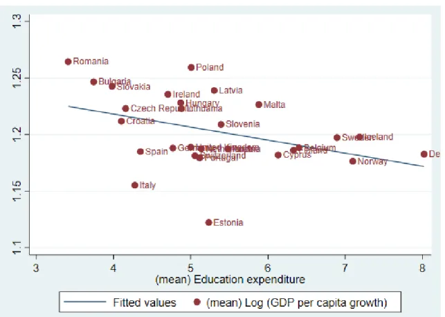
Figure 1 shows a clear negative relationship between the education expenditures and economic growth in the observed period, through the mean values of the variables. Thus, for example, Romania and Bulgaria, which on average have invested a modest amount of their GDP into education, have experienced relatively high economic growth in the observed period. Contrary, Norway, and Denmark have had relatively low growth rates on average in the observed period, despite their high investment into education.
6.1.2 School enrolment and economic growth
The second and third quantitative proxies of human capital used in this paper are school enrolment rates. More specifically, the secondary enrolment rate of males and the total tertiary enrolment rate are deployed as primary enrolment rates turned out to be
Figure 1: Mean logged values of GDP per capita growth plotted against mean values of education expenditure. Own calculations based on World Bank database from 1999-2019
insignificant at this stage of development (see Temple 1999, Barro 2001). For most of the EEA member states, secondary education participation is virtually 100% and changes over time have very little significance. However, the enrolment into tertiary education exhibits marked variability between the EEA countries and changes over time are obvious (see Table A1 in the appendix).
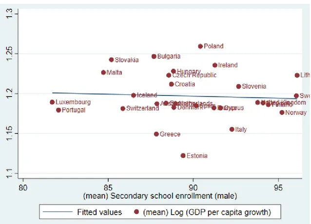
Figure 2 depicts the relationship between secondary school enrolment of males and growth in GDP per capita, based on the mean values of these two indicators in the observed period.
It is difficult to see any pattern between the variables in the figure. Namely, Poland and Ireland which have experienced relatively high growth on average in the observed period, have had high secondary school enrolment of males in the same period (as per expectations).
However, Malta and Slovakia had a mean growth rate that is higher than the EEA average growth rate for the observed period, while at the same time having secondary school enrolment rate of males on the level that is lower than the sample mean. Additionally, Norway and Sweden that have had males’ enrolment into secondary education on an
Figure 2: : Mean logged values of GDP per capita growth plotted against mean values of male secondary school enrollment. Own calculations based on the World Bank database from 1999-2019
extremely high level, have experienced, on average, low growth in this period. In the appendix (Figure A1), a visualization of the relationship between GDP per capita growth and tertiary school enrolment rates is provided. The conclusion does not differ much from the one concerning the enrolment rates into secondary education.
6.1.3 Years of schooling and economic growth
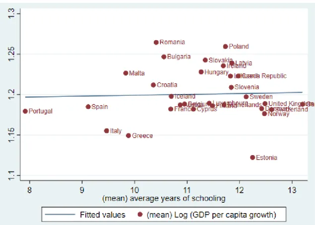
The fourth quantitative proxy of human capital in this paper is average years of schooling across all the educational levels. Even though this does not represent a perfect measure of human capital accumulation (see section 5.1), it is still a good approximation of that variable. Figure 3 shows a weak positive correlation between the average GDP per capita growth and mean years of schooling for the observed period. The outliers are Romania and Estonia, which have high and low average growth in GDP per capita in the observed period with relatively low and high values of average years of schooling in the same period, respectively.
Thus, the relationship between the average values of those 2 indicators seems to be in accordance with the expectations for the observed period.
Figure 3: Mean logged GDP per capita growth plotted against mean values of average years of schooling. Own calculations based on the World Bank database from 1999-2019
6.2 Regression Analysis
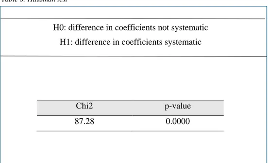
Before proceeding to the panel regression estimation of the main equation 11, it is crucial to decide whether to use a random effect or a fixed-effect model. Thus, the Hausman test is performed, and the results are reported in Table 6.
Table 6: Hausman test
H0: difference in coefficients not systematic H1: difference in coefficients systematic
Under the null hypothesis of the Hausman test, both random effect and fixed-effect models are appropriate. However, under the alternative hypothesis, only fixed effect estimation is an appropriate one. Since the chi2 value is 87.28 and its p=0, we can reject the null hypothesis and conclude that the fixed effect model is more suitable for this analysis.
To test for the presence of heteroskedasticity, the modified Wald test is performed, and the results are reported in Table 7.
Table 7: Modified Wald test for groupwise heteroskedasticity
Chi2 (31) p-value
15079.83 0.0000
Since the null hypothesis assumes the presence of constant variance (homoskedasticity), we can reject this and conclude that we have the presence of heteroskedasticity. To control
Chi2 p-value
for this, the robust standard errors are applied and adjusted for each of the analysed countries.
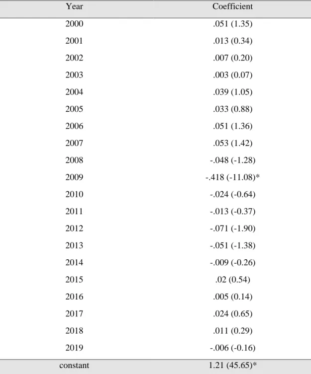
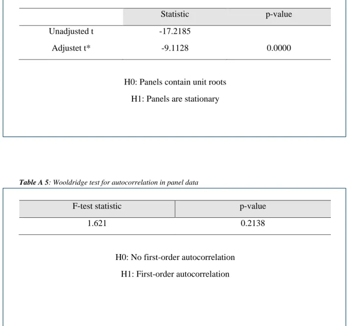
Additionally, tests for the stationarity as well as for the serial correlation are placed in the appendix (Tables A4 and A5, respectively). Based on the test results, it is concludable that we do not have a problem with serial correlation, neither with non-stationarity in the models.
Table 8: Fixed-effect panel regression with robust estimators
Variable Model 1 Model 2 Model 3 Model 4 Model 53
Constant 1.327 (4.92) * 1.098 (3.70) * 1.169 (4.43) * .8085 (2.41) * Government Consumption -.0295 (-4.64) * -.0301 (-5.3) * -.029 (-4.84) * -.0039 (-0.68) International Openness .0017 (1.42) .0012 (1.28) .0015 (1.34) . .0006 (1.63) Fertility Rate -.3218 (-2.86) * -.279 (-2.77) * -.285 (-2.84) * -.1585 (-4.9) * ln Investment Share .7054 (3.12) * .717 (3.15) * .6991 (3.13) * .61105 (2.86) * Inflation -.0004 (-0.21) -.0018(-0.41). -.0005 (-0.25). Years of Schooling -.0172 (-1.32) . Secondary Enrolment .0002 (0.3) Tertiary Enrolment . -.00009 (- 0.8) Education Expenditure -.0287 (-2.13) * Ln Inflation Rate -.041 (-1.75) Dummy 1 (year 2009) -.321 (-4.44) *
Ln initial GDP per capita -.05 (-2.71) *
Observations 588 610 593 439 651
R-sqr .198 .183 .1877 .503 .011
F-stat 7.57* 7.38* 7.58* 10.86* 7.36*
* Significant at 5% level of significance, t test values in parentheses
Source: Own calculations based on World Bank database from 1999-2019
Five different models have been deployed in this study. The first three models practically contain the same control variables, and the only notable difference is that each of them is using a different proxy measure for human capital accumulation.
Model 4, apart from the control variables that are used in the first three models, contains a dummy variable for the year 2009, in order to capture the expected negative effect of a great economic recession that was occurred in 2008. Additionally, the model also deploys the natural logarithm of inflation. These changes are made since they have led to the significant improvement of the model in terms of the higher value of R-squared, which is not that informative in the panel regression though, but more importantly in terms of the higher value of F statistics, which tests for the joint significance of the models.
The main reason for not including these changes in the first three models is due to the fact that there has not been any significant improvement of the models when those changes are made. The potential reason for this might be that education expenditures exhibit different patterns and have greater fluctuations in comparison to the other proxy measures (years of schooling, enrollment rates). However, since the literature on this particular issue is very scarce, this will mostly remain in the domainn of speculations.
Moreover, Model 5 is substantially different in comparison to the first four models, in terms of the specification as well as in terms of estimation method that is used for this model. Thus, it represents the regression of growth in GDP per capita on the initial level of this parameter, when all the other regressors are held constant. Furthermore, since the initial level of GDP per capita represents the time-invariant variable, it was not possible to include this variable in any of the first four models, as those have been estimated through the FE panel regression which only considers the variables that are time-variant within the countries. Consequently, that would result in omitting this variable from the models.
Hence, model 5 has been estimated through the Pooled OLS. The main aim of this model is to see if there is a convergence occurring in this economic area, which may make it more difficult to establish a meaningful relationship between human capital and economic growth.
Finally, it is also important to notice that all the models are statistically significant which we could see through their F statistics.
6.2.1 Effects of education
When it comes to human capital accumulation, measured through 4 different methods, and its impact on economic growth, the results might be slightly surprising. Namely, average years of schooling enter the equation with a negative coefficient, though it seems to be insignificant. This outcome might be due to several reasons. Hence, technical issues related to this way of capturing the effects of human capital are likely to influence and skew the results (see section 5.1). Furthermore, Correa, Jaffe and, Caicedo (2019) have showed that the predictive power of average years of schooling as a proxy for human capital started to dwindle in 1990 when the schooling of nations began to be homogenized. Having in mind that the EEA countries, which tend to have a relatively high degree of educational homogenization, are being analysed in the period after 1990, could clearly be a potential reason for obtaining the results like these.
The second and third proxy for human capital, the secondary and tertiary enrolment rates, appear not to have a different epilogue from the one that stands for average years of schooling. Thus, the estimated coefficient for secondary school enrolment takes on the value of .0008 and is insignificant (p-value=0.42). When controlling for the fertility rate, the coefficient is even decreasing to .0002 (p-value=0.82). These results might be due to the fact that all the EEA state members have extremely high enrolment rates into secondary education and changes over time have very little significance (see Descy and Tessaring 2004).
Moreover, the estimated coefficient of tertiary school enrolment is nearly zero and insignificantly enters the equation.
Finally, the third proxy for human capital, education expenditures that are spent in a particular year turned out to have a significantly negative effects related to economic growth in the same year, with a relatively low magnitude though (-.0287). However, by removing 2 outlying countries (Romania and Estonia) these effects become insignificant. This might be a proof of heterogeneity in the observed countries skewing the results as well as the implication that expenditures on education requires some time to manifest their positive effects, which will be the topic of section 6.4. Furthermore, imperfection of this way of measuring human capital that is already discussed in section 5.1 might be a reason for obtaining the results like these (see also Pelinescu 2015)
6.2.2 Effects of Control Variables
Government Consumption – The ratio of government consumption to GDP, represents
the measure of public expenditures that do not directly enhance productivity. In all the models (except for model 4 where it is controlled for education expenditure) this variable has a significantly negative impact on the annual growth in GDP per capita which is in accordance with the expectations. Furthermore, this negative impact is modest when it comes to its magnitude in all the models (an increase in government consumption by 10% points is estimated to reduce the growth rate by .3% per year in model 1)
International Openness- This measure represents the ratio of exports plus imports over
GDP. This variable enters the equation with a negative sign as per expectations but is insignificant. This most likely since the analysed countries belong to the same economic formation and thus have more or less uniform policies concerning the openness of their economies.
Fertility Rate- The estimates indicate that the growth in GDP per capita is significantly
negatively related to the fertility rate, and the magnitude of the coefficient is quite strong. An increase by 10% in fertility rate is estimated to reduce economic growth by 3.2 % in model 1. Thus, the decision to have more children per adult comes at the expense of economic growth.
Investment Share- The results indicate a significantly positive impact of investment on
economic growth as per expectations and the influence is very strong concerning the magnitude of the coefficient. Hence, in model 1, an increase by 10% in investment rate would increase economic growth by 7%, which is quite high.
Inflation Rate- Across all the models this variable enters the equation with a negative sign
but turns out to be insignificant at any conventional levels of significance.
Seasonal Dummy- in Model 4, the seasonal effect of the year 2009 is captured due to the
expected negative effect of the great recession that occurred in 2008 on economic growth. As per expectations, the dummy captures significantly negative effects of this year on the economic growth.
Initial GDP per capita- when all other independent variables from Table 6 are held
constant, there is a strong negative relationship between the growth rate and the initial level of GDP per capita.
4
In Figure 4 we could visualize this relationship. For the poorer countries of the EEA formation, the marginal effect of initial GDP might be positive. On the other side, for most of the richest countries of this economic formation, the effect of initial GDP on economic growth is strongly negative (Ireland obvious outlier). The estimated coefficient indicates that an increase in GDP by 10% points reduces the growth rate on average by roughly .5%.
This may be a proof of convergence occurring in this economic block, as poorer countries seem to be catching up.
4 note: the values plotted are normalized to make to make their mean value zero
Figure 4: Mean logged values of GDP per capita growth plotted against initial values of GDP per capita in 1999. Source: Own calculations based on the World Bank database from 1999-2019
6.3 The EEA countries segregation
Even though the observed countries belong to one of the highly developed economic formations, they still manifest a huge heterogeneity between themselves in terms of some of the important economic parameters (see Table 4).
Thus, instead of analysing it all together, as it is done in the previous section, it might be reasonable to divide these countries into several more homogenous groups based on some logical division criteria, which would potentially allow for capturing some patterns in a more visible and appropriate fashion. Hence, I have chosen the GDP classification, since the EEA member states exhibit significant heterogeneity when it comes to average GDP per capita in the observed period, which is shown in Figure 7.
Thus, 2 separate samples of countries are created based on the mean value of GDP per capita in the year 2019 which amounts to 40 541 US $ (see Tables A7 and A8 in the appendix). In group 1 are the countries with the GDP per capita values greater than the mean value whereas in group 2 are placed the EEA countries with the GDP per capita values lower than the mean value. The 2 groups are denoted as High-Income and Low-Income countries, respectively.
Figure 5: Comparison between the EEA countries based on the average GDP per capita in the period from 1999-2019.
The main goal of this division is to observe if there is a significant difference in the statistical parameters between the rich and poor countries of this economic area as well as to compare the results, especially ones related to educational effects, with the previous findings where all the countries were analysed at once.
Apart from the significant variation in the GDP per capita which was the main criterion for this classification, in Figure A3 in the appendix we could also see that on average, the richer countries of this economic block have higher average years of schooling as well as education expenditure in comparison to the poorer ones.
Table 9: Education effects comparison between the 2 groups
Human capital proxy High-Income Countries Low-Income Countries
(1)5 (2) (3) (4) (1) (2) (3) (4)
Years of schooling -.0024 (-0.6)
-.05 (-1.88)
Secondary school enrollment .001 (2.84)*
.003 (1.00)
Tertiary school enrollment .012 (2.64)* -.001 (-0.9) Education expenditure .007 (0.44) -.06 (-2.00) *
*significant at 5% level of significance *t test values in parentheses
In Table 9, estimated coefficients of 4 different proxy measures of human capital for both groups are reported. The full table with estimated coefficients of all other regressors from four models as well as R-squared and F test statistics are reported in Table A9 in the appendix.
Concerning the effects of education, it is clearly observable that education has a significantly different relation to the economic growth across the high-income countries in comparison to the poorer ones.
Years of Schooling - the estimated coefficient for this variable enters the equation with a
negative sign and is insignificant for both groups of countries.
Secondary School Enrollment - the estimated coefficient for high-income countries shows
a significantly positive effect of enrollment into secondary education of males on economic growth. However, when controlled for the fertility rate, the estimated impact turned out to be insignificant. On the other side, this proxy of human capital insignificantly enters the equation for the lower-income countries..
Tertiary Education- concerning this proxy measure, the estimated coefficient is showing
a significantly positive effect of tertiary school enrollment on economic growth for the upper GDP per capita group of countries. Thus, an increase in tertiary school enrollment by 10% is predicted to enhance economic growth on impact by .12 percent. However, this variable shows insignificant results for the lower GDP per capita group of countries.
Education Expenditure - the effects of the education expenditure spent in a certain year
on economic growth in the same year seem to be positive, though insignificant for the high-income countries. On the other side, it is estimated to have a significantly negative effects on economic growth of the countries on the lower levels of GDP per capita.
Furthermore, in Table A9 in the appendix, we may observe the impact of other regressors deployed in the models on economic growth across 2 groups. Thus, government consumption is estimated to have approximately the same negative effect on the economic growth of 2 groups. On the other hand, investment share and fertility rate, on average, have a significantly stronger positive and negative effects on economic growth, respectively, across the lower-income countries of this economic block in comparison to their richer neighbors. Namely, an increase in fertility rate by 10% is estimated to reduce the growth rate by 5% across the low-income countries whereas the same increase in fertility is associated with a 1.4% slowdown of economic growth across the high-income countries. This appears to be logical as richer countries tend to have a more developed mechanism for amortizing the negative effects of population growth (for example more developed technology). Furthermore, the stronger impact of investment on economic
growth across the poor countries is due to the rule of diminishing returns to capital, and as richer countries have higher levels of capital stock this finding seems to be in accordance with the expectations. Finally, international trade seems to be more important for the lower-income countries of this economic formation, whereas inflation is estimated to be insignificant in both of the groups.
6.4 Sensitivity check
Considering that the education expenditures are used as a proxy measure for human capital in one of the models, one might reasonably think of 2 issues in particular that are related to this way of measuring human capital accumulation:
• bi-directional effect (reverse causality) between the growth in GDP per capita in a certain year and public expenditure on education in the same year
• time-gap between the education expenditure and the effects that those provoke
The first potential issue is related to the fact that there might be reasonable to imagine education expenditure predicting growth in GDP per capita as well as all the way around. This occurrence could skew the reliability of the obtained coefficients.
Regarding the second potential problem, one may also argue that expenditure on education requires some time to impact the creation of human capital, and thus to have an influence on economic growth (activation period).
Thus, an ad-hoc method for dealing with these potential issues is performed by introducing a 1 year lag in education expenditure. This would allow for eliminating the potential problem of reverse causality as it is hard to believe that the education expenditure in year t-1 could be predicted based on the growth in GDP per capita occurred in year t, especially if we have in mind that GDP per capita growth does not suffer from the autocorrelation problem. Additionally, it would give some time for the effects of education expenditure to activate.
Table 10: Fixed effect panel regression using a 1 year lagged value of education expenditure Variable Full Sample
(EEA-28)6 High-Income Countries (EEA-12) Low-Income Countries (EEA-16) Constant .749 (1.88) 1.333 (4.63)* .3402 (0.61) Government consumption -.024 (-4.00)* -.032 (-6.64)* -.02 (-2.01)* International openness .0012 (1.69) .0002 (0.44) .002 (1.68) Fertility rate -.192 (-3.38)* -.108 (-2.32)* -.298 (-2.58)* Ln Investment share .734 (2.67)* .282 (2.44)* 1.076 (2.64)* Ln inflation rate -.019 (-0.71) .005 (0.25) -.064 (-1.37)
Lagged education expenditure (t-1) .0205 (1.32) .055 (5.85)* -.003 (-0.21)
F-stat 16.57 * 53.43 * 6.19*
R-sqr .2419 .3953 .2725
Observations 458 203 255
Cross sections 28 12 16
The model in which education expenditure is used as a proxy measure for human capital accumulation is performed again, yet this time with a 1 year lag in education expenditure. Furthermore, it is calculated for the whole sample as well as for the 2 subsamples separately, based on the same classification as in section 6.3.1 The results are reported in Table 9.
From the table, we may conclude that the investment in education that is done in the previous year positively, though not significantly, impact economic growth in the case where the whole sample is being analyzed. When we control for the impact of education expenditure in the current year (without-lag values) on economic growth, lagged value of education expenditure (t-1) becomes statistically significant with a magnitude of .056 implying that an increase in education expenditure in year t would enhance economic growth on impact by .6% in next year.
Moreover, when a subsample of more developed countries is analyzed separately, we may see a significantly positive effect of expenditure on education in the previous year on the economic growth in the next year. Thus, an increase in education expenditure in year t
6 Luxembourg, Greece and France are left out of the analysis due to the lack of data on education
would enhance the economic growth by .5% in the next year. When controlling for the current effect of education expenditure on economic growth in this group of countries, the coefficient of lagged education expenditure even increases in magnitude and takes on the value of .081.
Finally, when a less developed group of countries is taken into analysis, there are practically no effects of education expenditure done in a certain year on the economic growth in the next year. However, when controlling for the impact of current education expenditure, the coefficient of lagged education expenditure becomes positive (.0424) but statistically insignificant (p-value = 0.175).
Hence, we might conclude that education expenditure positively affects economic growth after some time lag (1 year in this study) in the case when the whole sample is analyzed. Furthermore, this impact is even bigger and statistically significant in the subsample of more developed countries, while there is no such an impact when less developed EEA countries are taken into account. This may suggest that above a certain stage of development, investing in education has a statistically positive impact on economic growth whereas at the lower stages of economical development education does not have that capability, likely due to the lower quality of those educational investments.