IN
DEGREE PROJECT TECHNOLOGY AND ECONOMICS, SECOND CYCLE, 30 CREDITS
,
STOCKHOLM SWEDEN 2018
Exploring the Relationship
Between Housing Prices and Stock
Prices
JOSEF AGUZ
OSSIAN MARKIEWICZ
KTH ROYAL INSTITUTE OF TECHNOLOGY
Exploring the Relationship Between Housing
Prices and Stock Prices
by
Josef Aguz
Ossian Markiewicz
Master of Science Thesis TRITA-ITM-EX 2018:228 KTH Industrial Engineering and Management
Industrial Management SE-100 44 STOCKHOLM
Master of Science Thesis TRITA-ITM-EX 2018:228
Exploring the Relationship Between Housing Prices and Stock Prices
Josef Aguz Ossian Markiewicz Approved 2018-06-08 Examiner Hans Lööf Supervisor Almas Heshmati Abstract
This study investigates the long- and short-run relationship between stock- and housing prices in Finland, Denmark, Norway and Sweden between 1987-2017 and 1995-2017 with data from OECD statistics. By using interest rate as a control variable and Johansen's Test for Cointegration, the results show a significant relationship for Finland during the period 1995-2017. The short-run analysis implies a credit effect, which is in line with previous studies. However, in Denmark, Norway and Sweden the analysis show no sign of cointegration. A possible explanation for the insignificant results could be the high degree of policy implementations and changes to market structures in the early 1990s, which theoretically could be controlled for by including additional control variables in the analysis.
Exploring the Relationship Between Housing
Prices and Stock Prices
Authors: Josef Aguz & Ossian Markiewicz
Supervisor: Almas Heshmati
May 31
th, 2018
Abstract
This study investigates the long- and short-run relationship between stock- and housing prices in Finland, Denmark, Norway and Sweden between 1987-2017 and 1995-2017 with data from OECD statistics. By using interest rate as a control variable and Johansen’s Test for Cointegration, the results show a significant rela-tionship for Finland during the period 1995-2017. The short-run analysis implies a credit effect, which is in line with previous studies. However, in Denmark, Nor-way and Sweden the analysis show no sign of cointegration. A possible explanation for the insignificant results could be the high degree of policy implementations and changes to market structures in the early 1990s, which theoretically could be con-trolled for by including additional control variables in the analysis.
Keywords: Housing Prices, Stock Prices, Cointegration, Credit Effect, Wealth Effect.
Acknowledgements
We would like to express our gratitude to our supervisor Professor Almas Heshmati for his useful comments, remarks and engagement through the learning process of this master thesis.
Contents
1 Introduction 4
2 Previous Studies 6
3 Theory 11
3.1 Consumption Theory . . . 11
3.1.1 The Permanent Income- and Life Cycle Hypotheses . . . 11
3.2 The relationship between markets . . . 13
3.2.1 The Wealth Effect . . . 13
3.2.2 The Credit Effect . . . 14
3.2.3 The Substitution Effect . . . 15
3.3 Statistical Theory . . . 15
3.3.1 Stationarity . . . 16
3.3.2 Augmented Dickey-Fuller’s Test . . . 17
3.3.3 VAR Model and Information Criterion . . . 18
3.3.4 Cointegration . . . 18
4 Method 19 4.1 Data and Transformation . . . 19
4.1.1 Housing Prices . . . 19 4.1.2 Stock Prices . . . 20 4.1.3 Interest Rates . . . 21 4.2 Presentation of markets . . . 22 4.2.1 Denmark . . . 22 4.2.2 Finland . . . 23 4.2.3 Norway . . . 25 4.2.4 Sweden . . . 27
4.2.5 Summary of policy implementations . . . 28
4.3 Testing for cointegration . . . 29
4.3.1 Step I - III: Determining order of integration . . . 29
4.3.3 Determining stability of cointegration . . . 30
5 Result 31 5.1 Results for order of integration . . . 31
5.2 Results for cointegration between 1987-2017 . . . 32
5.3 Results for cointegration between 1995-2017 . . . 33
6 Discussion 35 6.1 Significant cointegrated relationships . . . 35
6.2 Insignificant and unstable cointegrated relationships . . . 37
6.3 Conclusion . . . 40
6.4 Future Research . . . 40
7 Reference List 42
List of Figures
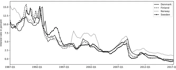
1 Development of Housing prices in Denmark, Finland, Norway and Sweden . . . . 19
2 Development of Stock prices in Denmark, Finland, Norway and Sweden . . . 20
3 Development of Interest rate in Denmark, Finland, Norway and Sweden . . . 21
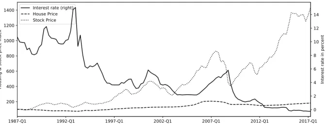
4 Development of Interest rate, Housing- and Stock prices in Denmark . . . 22
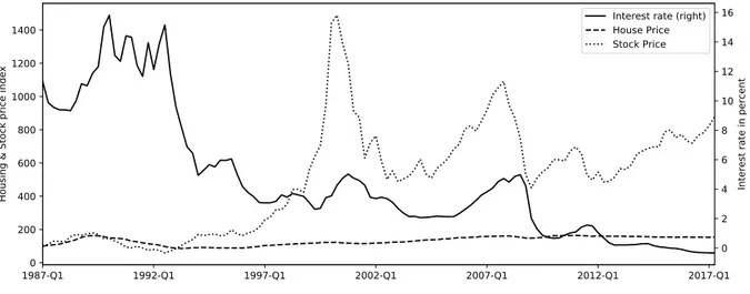
5 Development of Interest rate, Housing- and Stock prices in Finland . . . 24
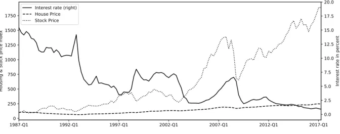
6 Development of Interest rate, Housing- and Stock prices in Norway . . . 25
7 Development of Interest rate, Housing- and Stock prices in Sweden . . . 27
8 Development of cointegrated Rtrend equation from 1995-2017 . . . 57
List of Tables
1 Previous studies on the correlation between stock and housing prices . . . 10
2 Overview of policy implementations for Denmark, Finland, Norway and Sweden . 28 3 Johansen test for cointegration in Denmark, period 1987 to 2017. . . 32
4 Johansen test for cointegration in Finland, period 1987 to 2017. . . 32
5 Johansen test for cointegration in Norway, period 1987 to 2017. . . 33
6 Johansen test for cointegration in Sweden, period 1987 to 2017. . . 33
7 Johansen test for cointegration in Denmark, period 1995 to 2017. . . 33
8 Johansen test for cointegration in Finland, period 1995 to 2017. . . 34
9 Johansen test for cointegration in Norway, period 1995 to 2017. . . 35
10 Johansen test for cointegration in Sweden, period 1995 to 2017. . . 35
11 Correlation of variables in Denmark, time period 1987-2017 . . . 48
12 Correlation of variables in Finland, time period 1987-2017 . . . 48
13 Correlation of variables in Norway, time period 1987-2017 . . . 48
14 Correlation of variables in Sweden, time period 1987-2017 . . . 49
15 Correlation of variables in Denmark, time period 1995-2017 . . . 49
16 Correlation of variables in Finland, time period 1995-2017 . . . 49
17 Correlation of variables in Norway, time period 1995-2017 . . . 50
18 Correlation of variables in Sweden, time period 1995-2017 . . . 50
19 Vector Autoregressive Estimation of Number of Lags, Cointegration Equation for time period 1987-2017, non-differentiated time series . . . 51
20 Vector Autoregressive Estimation of Number of Lags, Cointegration Equation for time period 1995-2017, non-differentiated time series . . . 51
21 Dickey Fuller test for time period 1987-2017, non-differentiated time series . . . . 52
22 Dickey Fuller test for time period 1995-2017, non-differentiated time series . . . . 52
23 Vector Autoregressive Estimation of Number of Lags, Cointegration Equation for time period 1987-2017, differentiated time series . . . 53
24 Vector Autoregressive Estimation of Number of Lags, Cointegration Equation for time period 1995-2017, differentiated time series . . . 53
25 Dickey Fuller test for time period 1987-2017, differentiated time series . . . 54
26 Dickey Fuller test for time period 1995-2017, differentiated time series . . . 54
27 Vector Autoregressive Estimation of Number of Lags, Cointegration Equation for time period 1987-2017 . . . 55
28 Vector Autoregressive Estimation of Number of Lags, Cointegration Equation for
time period 1995-2017 . . . 55
29 Johansen Test For Cointegration, period 1987-2017 . . . 56
30 Johansen Test For Cointegration, period 1995-2017 . . . 56
1
Introduction
During the last decades, there have been an upswing in research regarding the relationship between household wealth and consumer spending, due to the increase of volatility in stock market prices (Ali and Zaman 2017). The basis for the interest lies within the field of consumption theory, describing household spending (Ando and Modigliani 1963). In general, the theory implies that unpredicted changes in household wealth should have lasting effects on consumption behaviour. As unpredicted price increases in assets held by households will increase the consumption budget, an increase in consumption should occur and vice versa. (Paiella 2009) Since early research commonly viewed stocks as the greatest part of household wealth, focus was on the relationship between the stock market and household wealth. However, the results regarding the relationship was not consistent. The main explanation for this was attributed to the potential offsetting effect from the housing1 market. Hence, implying that households viewed housing assets as a part of
their aggregate wealth, therefore effecting current and future consumption. This was the beginning of a new approach, where studies focused on the relationship between housing-and stock prices. (Benjamin et al. 2004; Greenspan 2005; Paiella 2009)
To add to the complexity of the research area, the two assets differ in characteristics; housing can be seen as both an investment and a consumption good, as housing prices are determined by both demand and supply in a larger extend than stock prices. (Algieri 2013; Li et al 2017) Additionally, the characteristics of the two markets are also very different, where the stock market has low transaction costs, more liquidity and higher volatility. The housing market is considered to be more diverse and characterized with low liquidity and high transaction costs. (Ahangari and Moradi 2017) However, both assets are seen as common holdings of household wealth. Additionally, the difference between the two assets creates a potential risk diversification. (Li et al 2017; Lin and Fuerst 2014) Regardless if housing is viewed as an investment or consumption good, it is important to understand how housing- and stock prices influence each other.
Moreover, many factors need to be taken into account when examining this relation-ship. A true relationship between the two assets could be spurious due to effects from a third common variable. Additionally, the characteristics of the variables have to be
ex-1In the rest of this paper, the term ”housing” will refer to dwellings in form of houses and apartments.
amined in order to choose an appropriate statistical method. Furthermore, assuming that the two assets are seen as alternative investments, the relationship between housing- and stock prices should have non-linear characteristics. Since divergence between both assets in the long-run would not cause investors to change portfolio weights due to transaction cost, the two assets’ pace of price adjustment will differ. An additional argument for this would be that the difference in liquidity between the two assets could make investors delay changes in portfolio weights to avoid transitory shifts in prices. Hence, contributing to a non-linearity between the two asset prices. (McMillian, 2011) Thus, the two assets cannot be studied by only studying the correlation. Bozdogan (2018) recommend cointegration as an appropriate approach to investigate such dynamic relationship.
Generally, studies focusing on the relationship between the two assets have shown a positive interaction (Ibrahim 2010). Moreover, the direction of this causality has become more important for policy makers due to the price bubble phenomenon. (McMillian, 2011) However, there still exist different economic theories explaining various causality relations. One being the Wealth effect, where stock prices drive housing prices and the opposite, being the Credit effect, where housing prices drive stock prices. Thirdly, the Substitution effect explain how movements in both assets cancel each other out. (Li et al, 2017)
The geographical location and market structures can also contribute to differences across countries when it comes to the relationship between both assets (See Kapopoulos and Sioski 2005; Lean and Smyth 2013). Thus, it could be difficult to extrapolate result from one geographical area to another. One geographic area that lacks extensive research on the casual relationship is the Nordic countries. Given the current market conditions in the Nordic countries, it is appropriate to understand the relationship between both assets for these markets. The national increase in housing prices has accelerated the last few years in Denmark, Finland, Norway and Sweden and thus the possibility of a housing bubble may exist. The combination of growing disposable income for households and an extremely low interest rate across the countries have been the main explanation for this development. (Nordea Bank 2017) Additionally, both the Swedish- and the Norwe-gian Central banks reports how domestic housing prices has rapidly increased recently. (Riksbanken 2017; Norges Bank 2017) Furthermore, the Swedish Central bank state that equity prices also have increased and is now higher than prior to the financial crisis in
2008 (Riksbanken 2017). At the same time, the number of initial public offerings (IPOs) reached a new all-time high on the Nordic markets during 2017, implying growing equity markets. (EY 2017; Nasdaq OMX Nordic 2018).
In summary, the recent situation with broiling housing and stock markets in Denmark, Finland, Norway and Sweden, the purpose of this study is to investigate if housing- and stock prices are cointegrated in these countries by looking at both the short- and long-run effects. Thus, by answering this question, this paper intends to aid policy makers by contributing to the research field regarding the possibly interrelationship between both assets in the Nordic countries. In addition, there still exists conflicting economic theories on the subject of the causality between both assets. Therefore, with varying earlier empirical results, depending on countries and time period, and few studies focusing on the Nordic countries, this study would be an addition to the existing literature on the subject. By having insight about the relationship between these markets, policymakers in the Nordics will have the opportunity to adapt new policy implementations to the nature of the relationship, in order to achieve a sustainable economic development. Since both markets could affect household consumption and thus the level of economic activity in a country, the relationship is relevant for a long term economic sustainability.
The outline of this paper is as follows: Section two will provide a presentation of earlier studies investigating this relationship. Section three consists of a theoretical framework for the research question. The data and method used in order to answer the research question is presented in section four and the results are given in section five. The results are discussed in section six in relation to previous studies as well as the theoretical framework.
2
Previous Studies
The following section provides a selection of previous studies investigating the relationship between housing- and stock prices, with focus on different geographical locations, time periods, control variables and methods. A table summarizing the discussed studies are presented at the end of this section.
One of the earlier time periods examined was between 1973-1992 by Chen (2001) on the Taiwanese markets. By using a number of control variables and cross-sectional data, the study found a positive long-run relationship between the Taiwanese stock and
housing prices. The short-run analysis indicated that housing prices followed stock prices, implying that a wealth effect was present. The study also suggested that movements in stock and housing prices are better predicted by access to bank loans rather than a change in interest rate.
Ibrahim (2010) investigated the relationship between the assets in Thailand with data from 1995-2006 by applying Granger Causality Test and Impulse Response Function. Ibrahim (2010) also found a strong positive long-run relation between the two asset prices where stock prices drove housing prices in the short run, i.e. a wealth effect. The study concluded that stability in the stock market is necessary for a stability in the housing market.
Ahangari and Moradi (2017) looked at Iran with data from the same time period and used the same method as Ibrahim (2010). In line with Ibrahim (2010), they found a positive long-run relationship, where the impulse occurs in the stock price, every response of housing prices are positive. Hence supporting a wealth effect.
McMillian (2011), also found a long-run positive relationship between the assets when looking at the UK and US markets between 1974-2009. However, the short-run analysis suggested a relationship where housing prices drove stock prices, which support a credit effect. One explanation discussed was that rising housing prices allowed households and firms to increase consumption and investments, hence contributing to a rise in stock prices. (McMillian 2011)
Another study using data from UK was constructed by Ali and Zaman (2017). In-stead of focusing on just one market, the study examined data from 22 European countries between 2007 to 2012. Result was rather unanimous with a positive relationship in 15 countries and a negative relationship in five. Two countries, France and Italy, had insignif-icant results. In accordance with the above discussed papers, this study also established an overall short-run relationship where stock prices led house prices, in favour of a wealth effect.
One of the earliest cross-country studies was conducted by Quan and Titman (1999), including 17 countries from different continents. By using data from 1984 – 1996, the result suggested a positive long-term relationship between the two assets. However, the short-term relationship was insignificant and therefore hard to make a decision whether credit or wealth effect was dominating.
Another cross-country study was conducted around the same time by Sutton (2002), who investigated how house prices were affected by changes in national incomes, interest rates and stock prices. The results showed that all variables affected housing prices in the long-run. The short-run relationship suggested a wealth effect.
Kapopoulos and Sioski (2005) found it difficult to make a short-run analysis. By looking at the two markets in Greece, the result showed a long-run positive relationship. However, the relationship differed between regions, where stock prices drove housing prices in Athens while housing prices drove stock prices in other urban areas. Thus, both effects were present but in different parts of Greece.
Lean and Smyth (2013) also found differences when looking into specific areas. By using data from Malaysia, the authors did not find a long-run relationship between stock and housing prices. However, when narrowing the geographical location down to spe-cific areas and not looking at the country as a whole, the authors found a cointegrated relationship and evidence of stock prices leading housing prices.
By using rolling windows, i.e. dividing the observed period into sections, Li et al (2017) studied Chinese data from 2000 - 2016 and found both a present wealth and credit effect in China during this period but at different points in time.
However, few studies have used data from the Nordic countries. Sweden and Denmark were among the countries showing a positive relationship in Ali and Zaman’s (2017) cross-country study. Finland was solely in focus in a study made by Oikarinen (2010), by looking at data from 1970 to 2006. Oikarinen investigated whether the Finnish abolishment of controls on foreign ownership of stocks in 1993 had an effect on the relationship between the two assets. The results showed a long-run positive relationship between housing and stock prices both before and after 1993. A short-run relationship suggesting that house prices influenced stock prices, hence a credit effect.
In conclusion, most studies discussed above have found a positive long-run relationship between stock and housing prices. The majority of the research is in favour of a wealth effect (see Chen 2001; Sutton 2002; Ibrahim 2010; Lean and Smyth 2013; Ali and Za-man 2017; Ahangari and Moradi 2017). Contradictory, Oikarinen (2010) and McMillian (2011) find implications for the credit effect being dominant. While other studies found evidence of both effects being present, depending on point in time and regional areas (see Kapopoulos and Sioski 2005; Li et al 2017). Hence, as the results are mixed and research
focusing on Nordic countries is sparse, it exist room to contribute to the understanding about this specific geographic area.
Table 1: Previous studies on the correlation between stock and housing prices
Author(s) Geographical Location Time Period Control Variable Method Long-run Effect
Quan and Titman (1999) 17 countries* 1984-1996 CPI, GDP, Interest Rate, Cross-sectional Data Positive Insignificant
Chen (2001) Taiwan 1973-1992 GNP, Inflation, Money Supply Bivariate VAR, Granger Causality Positive Wealth
Sutton (2002) 7 countries** 1995-2001 GNP, Interest Rate VAR Positive Wealth
Kapopoulos and Sioski (2005) Greece 1993-2003 - Granger Causality Positive Credit/Wealth
Ibrahim (2010) Thailand 1995-2006 GDP, Inflation Granger Causality, IRF Positive Wealth
Lean and Smyth (2013) Malaysia 2000-2010 Interest Rate Cointegration, Granger Causality Positive Wealth
Oikarinen (2010) Finland 1970-2006 Foreign Ownership***, Tax Deductibility Cointegration Positive Credit
McMillian (2011) UK and US 1974-2009 - Cointegration Positive Credit
Ali and Zaman (2017) 22 Countries**** 2007-2012 - Cointegration, Granger Causality Positive Wealth
Li et al (2017) China 2000-2016 Inflation Continuous Wavelet Transform Positive Credit/Wealth
Ahangari and Moradi (2017) Iran 1985-2013 Exchange Rate, GDP, Inflation, Interest Rate Granger Causality, IRF Positive Wealth
*Australia, Belgium, France, Germany, China (Hong Kong), Indonesia, Italy, Japan Malaysia, Netherlands, New Zealand, Singapore, Spain, Thailand **Australia, Canada, Ireland, Netherlands, the United Kingdom and the United states ***Share of foreign ownership of the total value of the Helsinki Stock Exchange ****Austria, Belgium, Bulgaria, Croatia, Cyprus, Denmark, Estonia, France, Germany, Greece, Hungary, Italy, Latvia, Lithuania, Luxembourg, Malta, Poland, Slovakia, Slovenia, Spain, Sweden, and UK
3
Theory
This section will present theories relevant for the research area. Firstly, theories regarding consumption will be explained, focusing on the effects by changes in household wealth. Secondly, economic theory on the relationship between housing- and stock prices will be discussed. Lastly, statistical theory and framework used in this study will be presented.
3.1
Consumption Theory
According to Cooper and Dynan (2009), there are a number of reasons why fluctuations in housing- and stock markets might have a different effect on household wealth and therefore consumption. For example, housing could be seen as an investment asset, hence an increase in housing prices increase household wealth but also raise the price on other housing. On another note, the relative level of total mortgages as part of the housing asset will decrease and therefore create room to acquire additional debt. However, since the transaction costs on mortgages can be seen as high, households will increase the mortgage infrequently and therefore reduce the response of consumption as a consequence of housing price gains. (Cooper and Dynan, 2009)
Additionally, the financial structure in an economy can affect the consumption be-haviour. If the bank system is characterized with high down payment requirements, consumption may decrease in the case of a housing price shock, since individuals must in-crease their savings to afford the down payment to a new home. (Cooper and Dynan 2009) On the other hand, Ludwig and Slok (2004) found that consumption is more sensitive in “stock market oriented” economies. In this case, consumption should be less sensitive to changes in asset prices in countries with bank-based systems and less capitalized stock markets compared with countries characterized with high stock market capitalization. The discussion regarding the effect on consumption can be derived from two well dis-cussed theories, namely the Permanent Income Hypothesis by Friedman (1957) and the Life Cycle Hypothesis (Modiligiani and Brumberg 1954; Ando and Modiligiani 1963).
3.1.1 The Permanent Income- and Life Cycle Hypotheses
According to Friedman (1957), current consumption is based on future income, for ex-ample from wages, tax- and price changes and inheritance. Friedman summarized this
reasoning as the Permanent Income Hypothesis (PIH), proposing that consumption is based on estimations of future income. For example, the theory suggests that a student who borrows a lot of money for pursuing a university degree comfortably go into debt thanks to expectations of a high future salary, as a result of a university education. Thus, the expected future income could be seen a facility from which the student will draw down on, therefore only consuming marginally less during college than after, despite the difference in income. (Friedman 1957)
The theory also suggests that an individual’s consumption is ”smoothed” over a ca-reer, based on the expectation that a certain amount of money will be earned during a lifetime. Since wage levels are most likely increasing over time, “near-retirees” are usually at a lifetime income peak. In other words, the wage level will increase in line with the approach of retirement, but in the same time, the incentives for saving will increase due to the upcoming fall in income. This will contribute to a higher fraction of saving over time, in order to keep a constant consumption level after retirement. (Friedman 1957) Worth mentioning is that the “smoothing decisions” regarding consumption are based on information available to the individual at the point in time. If an unexpected positive income shock occurs, for example retaining a higher sales price on a house than expected, the individual is going to change current consumption behaviour, simply due to lack of prior information about this. The same reasoning can be used on negative income shocks, e.g. losses on the stock market, defaulted inheritance or health problems deterring the ability to earn wages. (Friedman 1957)
The Modigliani and Brumberg (1954) model suggests that the individual has the ambition to maximize its utility in relation to the available resources, being the sum of current net worth and future earnings. This later became the Life Cycle Hypothesis (LCH). However, in order for the utility theory to hold, Ando and Modigliani (1963) present five assumptions the theory is based on. The first assumption says that the utility function is consistent in relation to consumption at different points in time, meaning that an increase of resources in one period will be divided over different periods. Assumption two states that there are no expectations to receive inheritance or any attentions or desires to leave any inheritance. The third assumption says that the consumer always plan to consume the total resources evenly over all time. Assumption four suggests that every age group has the same average income at any given year. Hence, the expected average
income is the same in any age group. Additionally, every household has equal expected and actual total life and earning spans. The last and fifth assumption is that the rate of return on assets is expected to be constant and continuously be constant.
In conclusion, PIH and LCH are very similar, where LCH suggests that consumption is planed over a lifetime based on future income. While PIH states that individuals take on debt at a young age with expectations of higher income in the future and save during middle age to maintain the level of consumption after retirement. One main difference between the two hypotheses is that LCH pay more attention to saving and take account for both wealth and income when it comes to consumption. PIH on the other hand bring light on the individual expectations about future income and include inheritance as a variable for consumption behaviour.
3.2
The relationship between markets
The household sector can choose different approaches for saving money. Among the most common practices are saving money at a bank, invest money in financial markets or in housing assets. (Miles, Scott and Breedon 2012)
In line with LCH, Green (2002) suggests that a household consumption is mainly determined by income from labour and income from wealth (i.e. income from dividends or interest). The theory implies that households with high wealth can be expected, everything else alike, to consume more compared to households with lower wealth. Hence, if stock- and housing market returns are expected, wealth expectations are higher and therefore consumption should be higher. (Green 2002) Generally, three major theories can explain the causal relationship between the housing- and stock market; the Wealth effect, the Substitution effect and the Credit effect. (Li et al 2017)
3.2.1 The Wealth Effect
According to the wealth effect, there exists a one-way causality between housing- and stock prices, where the stock market influence the housing market (Li et al 2017). In more detail, a change in asset prices, i.e. stocks or housing, will affect the household’s net wealth and therefore its consumption. (Bernanke, Frank and McDowell 2006) However, this only holds if housing is seen as a consumer good. The price of consumer goods is determined by supply and demand and the supply of housing could be assumed to
be fixed in the short-run due to construction time. According to this reasoning, an increase in housing demand should boost prices on the housing market. (Li et al 2017) Moreover, expectations of future wealth will influence the current level of consumption (Case, Pollakowski and Wachter 1991).
However, since stocks cannot be seen as a consumer good and the stock market is assumed to be a random walk process, the wealth effect suggests that all changes in the stock market should be seen as permanent and unexpected. Therefore, an unexpected change on any of the markets will affect the net wealth of the household and in turn consumption. Thus, this will affect the demand for consumption goods and consequently housing prices. The wealth effect suggests that change in household wealth will not affect stock prices as they are an investment good and not a consumption good. Hence, investment levels are not affected by changes in net wealth. In summary, the effects of price changes run from the stock market to the housing market. (Li et al 2017)
3.2.2 The Credit Effect
According to the credit effect, there exists a one-way causality between housing and stock prices, where the housing market influence the stock market (Ibrahim 2010) A large part of firms’ assets consist of real estates. This means that a change in the value of a company’s real estates should change the value of the company, i.e. its value on the stock market. If the real estate value of a firm increases, the credit worthiness increases and the possibility to borrow money and invest more increase and vice versa. The credit effect also suggests that an increase in investments contributes to an increase in firm performance and thus its value. This in in line with Ibrahim’s (2010) description of the credit effect from a household’s perspective, where housing should be seen as a security or insurance. An increase in housing prices would give the household a better credit rating and therefore better access to favorable loans and a possibility to invest more both in housing and stocks. This can lead to increased consumption by households (McMillan, 2011). In summary, the effects of price changes run from the housing market to the stock market. (Ibrahim, 2010)
3.2.3 The Substitution Effect
According to the substitution effect, an increase in one of the markets should have a negative effect on the other market. Therefore, both assets are considered to be alternative investments to each other and illustrates that housing is a supplement to the stock market, i.e. the assets are substitutes. (Algieri 2013) This relationship can be economically interpreted as the substitution effect. In particular, if investors consider the stock market to be profitable, they will leave the housing market alone to focus on the more profitable market and therefore the demand for housing will decrease accordingly. (Shiller 2014)
A simple example to explain the substitution effect would be to consider a portfolio only containing stocks and housing assets. If the rate of return in the housing market becomes higher than in the stock market, the focus in investment will shift towards housing market (due to higher return). To be able to invest more in the housing market, some of the holdings in the stock market must be sold and will make stock prices decline. Hence, the housing market will go up even more but on the expense of the stock markets decrease. (Yin 2007)
However, since housing as an asset could be seen as less liquid than stocks, the effect from housing market to the stock market should be seen as weak in the short-run. In the long-run the housing market would have enough time to return to its long-run equilibrium and the investor would have enough time to re-balance the portfolio. (Li et al 2017; Yuan, Hamori and Chen 2014) In conclusion, the effect of price changes run between both assets with a negative effect. Hence, if one of the asset increase in price, the other asset will decrease in price.
3.3
Statistical Theory
The following section presents an overview of statistical theory necessary to answer the research question and to fulfill the purpose of this study. As previously mentioned, when studying the relation between variables in this setting, the potential presence of non-stationary variables and spurious relationship have to be considered. Thus, a regression between variables could show a significant result, when in reality there exist no underly-ing relationship. Hence, the result does not have a real economic value. (Granger and Newbold 1974) A method presented by Engel and Granger (1987) avoids this problem
and enabling inference of the relationship between non-stationary time series without loss of data. In order to do so, certain assumptions must be fulfilled. (Engle and Granger, 1987) This is further discussed below.
3.3.1 Stationarity
A stationary variable is not explosive or drifting aimlessly without returning to its mean. In other words, a covariance-stationary time series Yt is portrayed by a constant mean,
E(Yt) = µ, (1)
for all t and a constant covariance,
Cov(Yt, Yt−k) = γt, (2)
which holds for all t. Where the covariance is only dependent on the lag length, represented by k. Consequently, this gives the property of constant variance,
V (Yt) = σ2, (3)
for all t. These characteristics contribute to a series with a mean-reverting feature, resulting in a time series that will fluctuate around it long-term mean value over time. From now on, such process will be referred to as a stationary series. To deeper clarify stationary and non-staionary time series a first order autoregressive (AR) model can be used,
Yt= φYt−1+ ut, (4)
where Ytis explained by its lagged component, Yt−1with the coefficient φ and ut, which
is an independent and identically distributed random variables, (0, σut). By expanding
the Yt−1 to an infinite moving average process, MA(∞),
Yt = ut+ φut−1+ φ2ut−2+ φ3ut−3+ ..., (5)
is obtained. The effect of the error term will disappear over time if |φ|<1. This is a vital assumption for a stationary series with a mean-reverting property. However, if φ = 1 the effect of a ut−k would never vanish, which will imply a non-stationary time
series with no mean-reverting properties. Series with such characteristics is called a unit-root process, i.e. a random walk in economic terms. A random walk is basically the movement of variables with a random pattern over time. Due to the fact that the variable follows an unpredictable course, forecasting future paths cannot be done by looking at previous data.
However, a non-stationary series can become stationary by taking the first difference and repeating the process until it is stationary. A series that becomes stationary after d repetitions are said to be integrated of order d, with notation I(d). (Asteriou and Hall 2011)
3.3.2 Augmented Dickey-Fuller’s Test
This test looks for the existence of a unit-root in the time series i.e. determining existence of a non-stationary series. The model,
∆yt = γyt−1+ p
X
i=1
βi∆yt−i+ ut, (6)
is fitted to the data with the null hypothesis H0 : γ = 0 (non stationary) and Ha :
γ<0 (stationary). If the null hypothesis is not rejected in equation 6 where the coefficient γ = (φ − 1), it suggests that γ = 0 which is only possible if φ = 1. As a result of this, the time series has a unit-root process. The test statistic is obtained by a t-test,
ADFobs = ˆ γ ˆ σγ (7) and the calculated value is compared to the Dickey-Fuller’s distributions critical value. Two additional models can be used, depending on the characteristics of the time series:
∆yt = α0+ γyt−1+ p X i=1 βi∆yt−i+ ut, (8) and ∆yt = α0 + α1t + γyt−1+ p X i=1 βi∆yt−i+ ut, (9)
where the intercept α0 represents a non-zero mean in the time series where α1t allows
3.3.3 VAR Model and Information Criterion
The vector autoregressive (VAR) model is a multivariate model with the characteris-tic of not differentiating between exogenous and endogenous variables. Each variable is modelled with its lagged values, corresponding to the value in prior period (t − 1). It is essential to specify each models number of lags correctly. Too few lags can lead to specification errors and using too many lags can result in multicollinearity. (Asteriou and Hall 2011) The accurate number of lags can be determined by approximating k number of VAR models, where the largest model has k lags. Four information criterion’s is es-timated for each model. In this investigation, Sequential likelihood ratio (LR), Akaike-(AIC), Hannan-Quinn- (HQIC) and Swarts Bayesian- (SBIC) is used. The appropriate lag length is found by selecting the model which minimize the value of the information criterion. (Asteriou and Hall, 2011)
3.3.4 Cointegration
If two or more time series are cointegrated, there exists a long-run relationship and a long-run equilibrium value between the series. It does not necessary have to exist an equilibrium in the short-run between the time series, but they will always converge in the long-run. (Asteriou and Hall 2011) For instance, if three time series are integrated of order Xt ∼ I(b), Yt ∼ I(d) and Qt ∼ I(c) where b = d = c are said to be cointegrate if
there exists a linear combination of the three that is stationary in itself, such as ut in
Qt− θ1Yt− θ2Xt= ut∼ I(0). (10)
If these series are cointegrated the variables θ1 and θ2 are entitled the cointegrated
coefficients and a long-term relationship exists. Hence, there exists a mean returning property and the variables would, over time, convert back to the equilibrium if they divert from their long-term mean. In an equation with n number of variables there can exist up to n − 1 cointegrated relationships. Johansen’s proposed test for cointegration will be used in this investigation.2
2The specifics of the vector autoregressive approach and the relationship between its eigenvalues and
the rank of its matrix or the vector error mechanism will not be discussed in this paper.
4
Method
This section will start by presenting the data, its source and how it has been transformed. Further, a short description of economic events linked to each data variable and market is presented. Lastly, the method used to test for cointegration is defined.
4.1
Data and Transformation
All data is collected from OECD statistics website3 on January 18, 2018. All variables for
Finland, Denmark, Norway and Sweden are observed quarterly from Q1:1987 to Q2:2017 with 118 observations each. Furthermore, all variables are transformed by natural loga-rithm to enable more normally distributed error terms since this is assumed in the applied method. The time period was chosen due to the availability of relatively long time series of housing prices at a quarterly frequency. The variables are described with OECD’s statistics definition.
4.1.1 Housing Prices
For all countries price levels are index at 100 in 1987 Q1.
Figure 1: Development of Housing prices in Denmark, Finland, Norway and Sweden
This study use the hedonic price index RPPI (Residential Property Prices Indices) from OECD statistics, as recommended by Hill (2013). The hedonic index is obtained by the hedonic regression, it accounts for locations, specific characteristics of the individual
objects and housing costs; rent prices, real and nominal house prices, and ratios of price to rent and price to income. The index uses 2010 as the base year. (Hill, 2013; OECD A 2017 ) This study specifically use the Real House Prices which is based on the ratio of nominal price to consumers’ expenditure deflator as it has been commonly used in most previous studies (e.g. see Oikarinen, 2010; Chen, 2001; Ibrahim, 2010; Ahangari and Moradi 2017).
4.1.2 Stock Prices
For all countries price levels are index at 100 in 1987 Q1.
Figure 2: Development of Stock prices in Denmark, Finland, Norway and Sweden
The Stock Price variable is calculated from the common company shares traded on both national or foreign stock markets. The value is determined by the stock exchange and expressed as a simple arithmetic average of the quarterly data to form an index. The Share Price index measures the market capitalization of the basket of shares. (OECD B 2017)
4.1.3 Interest Rates
Figure 3: Development of Interest rate in Denmark, Finland, Norway and Sweden
When studying the relationship between stock and housing prices, one must reflect whether an external variable can affect the price levels. Using a control variable, one could avoid a false relationship between these variables. (Quan and Titman 1999) The interest rate is of favourable character due to its influence of a household’s cost of loans as well as the choice between saving money in a bank account versus investing on the stock market. Therefore, interest rate should have a significant effect on both stock- and housing prices. Thus, the level of the interest rate should to some extend reflect the price level on mar-kets. (Miles, Scott and Breedon 2012). As an example, a low interest rate contributes to a lower cost of borrowing, making it cheaper to invest in housing or on the stock market. Additionally, a low interest rate make it less beneficial to save money in a bank account due to lower return. Therefore, in this case investments and consumption should increase, given an unexpected decline in interest rate. (Sutton 2002) This also accounts for interest rates relationship with stock prices, where a low interest rate makes it less beneficial to save money at a bank, hence making the stock market a good substitute. (Ahagari and Moradi 2017) Hence, interest rate should have a negative relation with both stock- and housing markets.
This study uses the variable Short-term interest rate from OECD statistics, repre-senting the rates of short-term borrowings between financial institutions or the rate at which short-term government bonds are traded in the market. The variable is based on average quarterly rates that are measured as a percentage and based on three-month
money market rates. (OECD C 2018) Additionally before transforming the variable by natural logarithm, every observation is first transformed by adding ”1” in order to enable transformation of the negative values.
4.2
Presentation of markets
In this section, the economic developments of importance for this research are reviewed for each of the examined markets; Denmark, Finland, Norway and Sweden.
4.2.1 Denmark
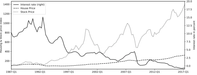
In the mid 1980s the Danish economy was characterized by high unemployment and inflation, combined with high government budget deficits. In early 1980s the decision was made to not devalue the Danish Krone and furthermore to turn to a fixed exchange-rate policy. This led to higher nominal interest rate to protect the exchange-rate. However, Denmark experienced lower real interest rates during the same period, in turn driving up house prices, consumption and the demand for loans. To dampen the issuance of new loans, a policy was introduced in 1987 that significantly reduced the benefits from tax deductions on interest rate. However, this had a larger impact than expected on housing as can be seen in house price decline from 1987 to about 1993 in the graph below. (Abildgren, Andersen and Thomsen 2010)
Housing- and Stock price levels are index at 100 in 1987 Q1, measured on left axis. Interest rate is percentage point, measured on right axis.
Figure 4: Development of Interest rate, Housing- and Stock prices in Denmark
In 1988 the final restrictions on capital movement to and from Denmark was lifted,
resulting in more foreign investments in the country, followed by a three-year increase in stock market prices. At the start of the 1990s the Danish Government experienced the first year with a budget surplus for the last 25 years. However, to combat the banking crisis of the early 1990s the Danish government eased the capital requirements for banks, in order to enable easier loss absorption. In 1993, the Danish Bank pledge to defend the current rate of Danish Krone. However this marks a period in the 1990s with the largest currency unrest to date, as can be seen in the high volatility of the interest rate around 1993. In the end of the 1990s Denmark agreed on locking their currency to the Euro (EMR II).
During the mid and later part of the 1990s, adjustable rate loans was introduced, combined with tax cuts for housing assets and declining mortgage rates, this fueled the housing market up until 2004. The same year Denmark experienced an increase in unem-ployment, resulting in introduction of new fiscal policies in order to stabilize the economy. The fiscal policies contributed to a decrease in unemployment which went below 2 per-cent in 2007. This has been proposed as the main reason for consumer’s higher confidence which lead to higher stock- and house prices as well as higher consumption. (Abildgren, Andersen and Thomsen 2010) In late 2007, Denmark was affected by the global financial crises, where housing- and stock prices fell in last quarter of 2007. This was a result of strong lending growth the years prior to the crisis and the Danish government had to intervene to save banks. (Abildgrenand and Thomsen 2011) However, housing prices have started to slowly recover, closing in on pre-crisis price levels. While share prices have grown well past crisis levels and are on all time high currently. Due to the crisis and European interest rate (i.e EMR II affiliation) the Danish interest has trailed towards zero during the last years. (ECB, 2018)
4.2.2 Finland
The most important economic event related to housing market in Finland occurred be-tween 1987-1989 where prices rose by more than 60 percent in about two years. The rise was attributed to deregulation of financial markets, leading to increased access to capital. When the bubble burst the correction in prices continued for the following four years, as can be seen in the graph below. (Kivist¨o 2012)
Housing- and Stock price levels are index at 100 in 1987 Q1, measured on left axis. Interest rate is percentage point, measured on right axis.
Figure 5: Development of Interest rate, Housing- and Stock prices in Finland
To combat the sudden response to the deregulation, Bank of Finland started with open market operations in 1987 and bought government securities in order to contract the amount of money in the Finnish banking system. The collapse of the Soviet Union in 1991 led to a decline in Finland’s export trade, thus deepening the depression. (Bank of Finland 2015) Later in 1993, Finland abolished the control on foreign ownership of stocks (Vaihekoski 1997). Finland had a high export during the 1990s and it was further boosted by the entrance to European Union in 1995 (Bank of Finland 2015).
However, just after the peak in export around 2000, Finland’s economy was effected by the IT bubble, where the overall demand decreased and brought an end to the booming Finnish export. The sharp increase and decline was highly influenced by the fact that the IT company Nokia, at its peak in 2000, constituted for about 70 percent of the total market cap of Helsinki Stock Exchange (Oikarinen 2010).
In 2007, the Finnish housing prices increased and the stock market reached a peak due to increases in exports (Laitam¨aki and J¨arvinen 2013). Additionally, household consump-tion was historically high. The years before the financial crisis in 2008, consumpconsump-tion was higher than disposable income, meaning households spent more than the household in-come due to easy access of loans. (BOF Bullentin 2017) Consequently, when the financial crises of 2008 occurred, the Finnish stock market experienced a drastic decline and fell between 2007 and 2009. (Laitam¨aki and J¨arvinen 2013) At the same time, not tied to the financial crises, the important domestic mobile phone sector experienced further decline in exports. This event further deepened the negative effect on the Finnish economy. (Bank
of Finland 2015) As can be observed in the graph, the stock market price has slowly re-covered but has not reached pre-crisis levels. After the financial crisis, the unemployment rate increased, which contributed to monetary policies favouring a lower interest rate to boost the economy. As a result of lower interest rates, housing prices increased and soon reached pre-crisis levels again. (Kuuster¨a and Tarkka 2012) Since late 2014, the savings ratio has actually been negative again, thus indicating a repeating fragile consumption behaviour. Underlying contributing factors to consumption growth include the low inter-est rates and strengthened consumer confidence. Both factors encourage households to increase consumption and reduce saving. (BOF Bullentin 2017)
4.2.3 Norway
In the mid 1980s the Norwegian housing market was characterized by high degree of rental apartments with regulated rents. During the same time, the government started deregulation of the credit market and introduced favourable tax rules for interest costs. Furthermore, during the same period Norway saw a high degree of economic activity and low real inflation. Consequently, the country experienced an increase in the credit supply, which resulted in a substantial increase in relative housing prices in 1985. (Stamso 2009) In 1986 the Norwegian government handed over the governance of the short-term interest to the Norwegian Central Bank (Norges Bank 2018). Due to uncertainty in the international stock market coupled with an oil price decline and high inflation, the start of the collapse in housing prices begun in 1988 (Stamso 2009) as seen in Figure 6 below.
Housing- and Stock price levels are index at 100 in 1987 Q1, measured on left axis. Interest rate is percentage point, measured on right axis.
The central bank responded with increasing short-term interest, trying to stabilize the Norwegian Krone (Norges Bank, 2018). In the end of the 1980s, the housing market started to be liberalized and a beginning of a transformation of rental housing to commer-cial real estate commenced. During the same period, Norway experienced a Bank crisis, largely due to bad performing loans issued after the deregulation of the credit market. (Stamso 2009) In 1990, the Norwegian Krone was pegged to the European Currency Unit (ECU). However, as a result of the turbulent currency markets of 1992, it was decided to abandon the link to ECU. The same year the inflation target was set at 2.5 percent for Norway’s Central Bank and the economy experienced a great fall in interest rate, bene-fiting home owners with outstanding loans. This started a steady appreciation in house prices for Norway after previous years decline. (Norges Bank 2018)
For most part of the 90s the government continues with further deregulations of the housing market. (Stamso 2009) Norway is mostly unaffected by the IT-crisis in 2000 compared to its neighbouring nations, with a small drop in stock prices and stagnating house prices. Following the short-run decrease in stock prices the stock market starts on sharp rise due to the sudden increase in oil prices, continuing as far as the financial crisis of 2007. (Bank of Finland, 2015) Household consumption increased significantly between 2005 and 2014. In the years prior to the financial crisis, total consumption expenditure was above total disposable income. However this changed after the crisis but consumption still remained high. (Lindquist, Solheim and Vatne 2016) Following the crisis, the Finance Department decided to regulate Banks after prior deregulations, mainly focusing on increasing capital requirements to stabilize the financial system. (Norges Bank 2018)
Due to the deregulation and new policy targets the real estate market in Norway have changed drastically. In 1987, the market was characterized by low degree of home ownership, but with a transition to a high degree of home ownership, Norway had the highest degree of home ownership in the Nordics by 2009. Thus, in the time period from 1980 to 2009 Norway went from a social democratic characteristic housing market to a more liberalistic one. (Stamso 2009)
4.2.4 Sweden
In 1985, the Swedish central bank started to deregulate the financial market and open it up for foreign investments, following the trend of internationalization of stock markets around the world. Simultaneously, the previous loan cap and interest rate regulation was abolished, contributing to better access to loans, consequently leading to rising housing and equity prices. (Riksbanken A 2018) This continued throughout the 1980s, as can be seen in Figure 7 below.
Figure 7: Development of Interest rate, Housing- and Stock prices in Sweden
As a result of the global crises in 1987, the central bank’s independence from the government increased. By 1991 the Central bank decided to peg the Swedish currency to the European Currency Unit (ECU). As a result of the international economic downswing and currency volatility, the Swedish currency starts to decline in the beginning of the 1990s. In an attempt to defend the exchange rate, the interest rate was set to 500 percent in 1992, in order to deter the Swedish currency from floating out of the country. However, the attempt failed and the Swedish Central Bank soon lowered the interest rate and the exchange rate fell as a result. The following years the inflation target was set to 2 percent (Riksbanken A 2018) and the Swedish Central Bank introduced the Repo rate as the main tool to control money supply. (Riksbanken B 2018) In 1995 Sweden joins EU (Riksbanken A 2018) and the following years the Swedish stock trading increased until the end of 1990s. (Nasdaq OMX B 2018)
The global financial crisis in 2008 contributed to OMXSPI’s largest fall since the beginning of the 1990s (Nasdaq OMX B 2018). Yet, Sweden was considered to have
coped well, thanks to learnings from the early 1990s crises (Riksbanken A 2018). Sweden faced a fall in inflation the following years and in order to bring the inflation level up, the Repo rate was set to zero percent in 2014. This was a historically record low interest rate but the effects were smaller than expected and a negative rate was introduced the following year. The extreme low interest rate contributed to an easier access and more beneficial mortgages for households and thus the housing prices increased. In 2016, a new aggressive amortization requirement was introduced to battle the increasing debt ratio of households. (Regeringen 2016)
4.2.5 Summary of policy implementations
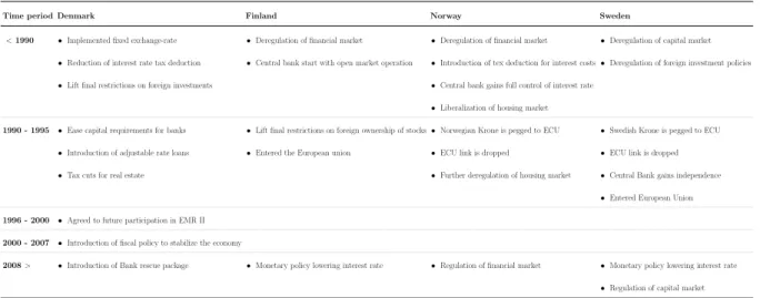
Table 2 below show an overview of policy introductions for the chosen period for each market.
Table 2: Overview of policy implementations for Denmark, Finland, Norway and Sweden
Time period Denmark Finland Norway Sweden
< 1990 • Implemented fixed exchange-rate • Deregulation of financial market • Deregulation of financial market • Deregulation of capital market
• Reduction of interest rate tax deduction • Central bank start with open market operation • Introduction of tex deduction for interest costs • Deregulation of foreign investment policies
• Lift final restrictions on foreign investments • Central bank gains full control of interest rate
• Liberalization of housing market
1990 - 1995 • Ease capital requirements for banks • Lift final restrictions on foreign ownership of stocks • Norwegian Krone is pegged to ECU • Swedish Krone is pegged to ECU
• Introduction of adjustable rate loans • Entered the European union • ECU link is dropped • ECU link is dropped
• Tax cuts for real estate • Further deregulation of housing market • Central Bank gains independence
• Entered European Union
1996 - 2000 • Agreed to future participation in EMR II
2000 - 2007 • Introduction of fiscal policy to stabilize the economy
2008 > • Introduction of Bank rescue package • Monetary policy lowering interest rate • Regulation of financial market • Monetary policy lowering interest rate
• Regulation of capital market
Overall, all four markets experienced housing crises in the late 1980s due to deregu-lations of financial markets. This was followed by different aggressive monetary policies. The 1990s was characterized with policies followed by the establishment of the European Union. Except the IT crisis during the late 1990s, the housing and stock market begun to bloom again in line with low interest rates. The buildup ended with the financial crises of 2007-2008, where new policies was introduced to stabilize the economies.
4.3
Testing for cointegration
This study’s method will follow the approach suggested by Johansen (1995) to accompany the cointegration analysis. In Johansen’s step-by-step approach, I: for each time series, the correct model has to be specified in terms of trends and intercepts. II: the optimal lag length is determined by estimation of VAR-model for each variable. III: the order of integration for each variable is determined. IV: the optimal lag length is estimated for the possible cointegrated equation. V: finally, the number of cointegrated equations is estimated.
4.3.1 Step I - III: Determining order of integration
First, for each time series the correct model has to be specified, determining possible linear trends or intercepts for the ADF-test (see section 3.3.2). In line with Hendry et al. (2001), the model specification is done by graphical analysis combined with theory based reasoning, since the specification could vary between different time series.
Secondly, for each time series the optimal lag length will be estimated by VAR-models. Lag length is determined by using the Sequential likelihood ratio (LR), Akaike- (AIC), Hannan-Quinn- (HQIC) and Swarts Bayesian- (SBIC) information criterion for estimated VAR-model. Moreover, lower number of lags will be favored, as such models are preferred due to issues with over specification (Juselius, 2006).
Thirdly, by using Augmented Dickey-Fuller test the order of integration is determined. This is done by first testing for a unit root in the original time series and then repeating the process for the differentiated one. If the first test fails to reject the null hypothesis of non-stationarity and the second test is rejected, the time series are integrated of the first order. Given that all-time series are integrated of order one for a country, it is possible to proceed to estimate the existence of a cointegrated relationship.
4.3.2 Step IV - V: Determining existence of cointegration
In step IV, the prior steps I and II is repeated for the possible cointegrated equation. Moreover, in model specifications for the cointegrated equation there are four common models. Model 1: where no restriction is used on either intercept or trend, resulting in an equation which is stationary with a quadratic trend. Model 2: where the trend is
restricted to a linear trend and the constant is not restricted, resulting in a stationary process with a linear trend. Model 3: in this model the trend is fully restricted with an unrestricted constant, resulting in a process that is stationary around a constant mean. Model 4: in this model both the trend and constant is restricted, yielding a cointegrated relationship centered around zero.
Further, in the case of time series variables which are trend stationary, as is most com-mon for asset prices, model 2 has comcom-monly been used while the other have been deemed ill suited for common use. (Ahking, 2002; Juselius, 2006; Oikarinen, 2010) However, model 2 implies that the returns between both assets are growing at the same rate, while for the countries examined in this study growth of stock prices have exceed the growth of housing prices. Oikarinen (2010) and McMmillan (2011) argues for using model 1, thus also allowing the trend to be unrestricted. This would enable the cointegrated relation-ship to have a quadratic trend while it is still trend stationary. Even though model 1 has not commonly been used in this research field, the assumption of equal growth rate between the variables is deemed to be a stricter assumption compared to allowing one of the variables to grow at a higher rate.
As a result, this study will include both model 1 and 2 when testing for cointegration. Lastly in step V, the Johansen’s test is performed using the trace statistic. From this the long-run cointegrated equation and the short-run correction parameters are estimated.
4.3.3 Determining stability of cointegration
When a cointegrated equation is determined, the stability of the estimation have to be tested (Juselius, 2006). Firstly, all the short-run adjustment coefficients have to be neg-ative or close to zero. This is important as it enable the system to reach and sustain a long-term equilibrium. If the system would experience a shock to one of the variables, the negative adjustment parameters would allow the system to return to its equilibrium. The equilibrium could be centered around a new level, depending on if the constant in the equation is unrestricted. Furthermore, the cointegrated equation is sensitive to auto-correlation and non-normally distributed errors (Juselius, 2006).
To confirm that the cointegration equation itself is stationary, ADF-test is used. The predicted values are also visualized to understand the movement of the cointegrated equa-tion over time. Jarque-Bera test is used to test the normality assumpequa-tion of the errors
terms in the VECM (Jarque and Bera 1980). If the Jarque-Bera test fails the skewness and kurtosis is estimated to provide a deeper understanding of the distribution of errors. Lagrange Multiplier test is used to determined possible autocorrelation of error terms in the estimated VECM (Johansen, 1995).
5
Result
In this section, the result from the performed tests will be presented. First, the results on tests with data from the period Q1:1987 - Q2:2017 will be displayed. Secondly, due to the high degree of monetary reforms in the countries in the period 1987 to the mid 1990s (see section 4.2) a second analysis is performed between Q1:1995 - Q2:2017, using a subset of the same data set.
5.1
Results for order of integration
The graphs for each variable and country is examined to determine the correct model for the ADF test, that fit the data in combination with economic reasoning (see Figure 1, 2 and 3 in section 4.1). For house and stock variables, the characteristics of the data for Norway, Sweden and Denmark has a trend component. This is in line with the economic assumption of positive returns for both house and stock assets over time (Oikarinen 2010). In Finland, both variables’ data characteristics indicate a non-trend process allowing for non-zero mean i.e. an intercept in the test model. However, this contradicts the general assumptions described earlier as a result of this both models will be applied for housing and stock prices in Finland.
Regarding the interest rate variable for all markets, the data characteristics show a negative trend in the time series. However, from a theoretical view point, allowing for a trend component would not hold over time, as this would result in a continuous decrease in interest rate. Thus, this study assumes interest rate to have a non-zero mean without any trend component. After determining optimal lag length for each time series all the variables are determined to be integrated of order one on a significance level of five percent. Thus, the first assumption for Johansen’s cointegration test is fulfilled.
5.2
Results for cointegration between 1987-2017
For the cointegration test, the lag length estimation gives multiple suggestions for optimal lags (see Appendix table 19 and 20). Thus both suggestions will be used in this analysis. First, the analysis is done for the full time period from Q1:1987 to Q2:2017, using all suggested lag lengths and applying both model specifications for the cointegrated equation, as can be seen in Table 3, 4, 5 and 6 below.
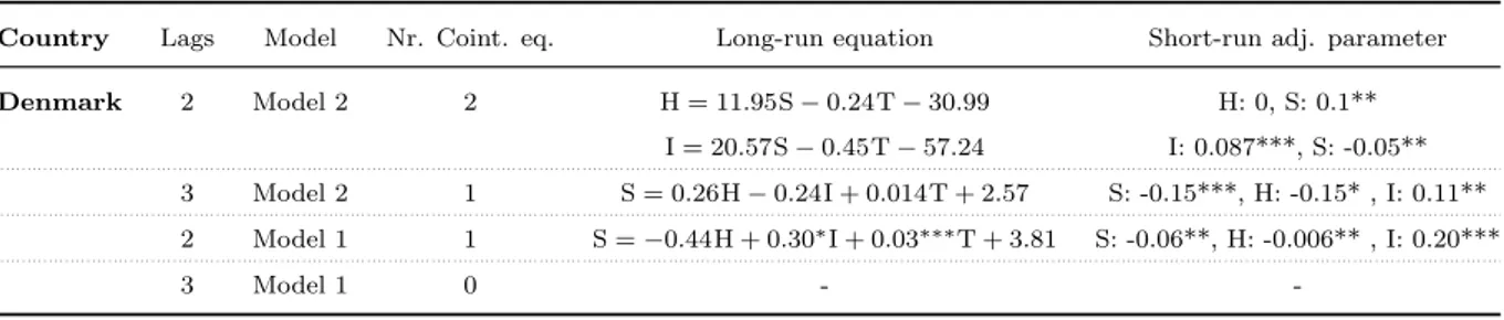
Table 3: Johansen test for cointegration in Denmark, period 1987 to 2017.
In the table housing prices are represented by H, stock prices by S and the interest rate is represented by I.
Country Lags Model Nr. Coint. eq. Long-run equation Short-run adj. parameter Denmark 2 Model 2 2 H = 11.95S − 0.24T − 30.99 H: 0, S: 0.1**
I = 20.57S − 0.45T − 57.24 I: 0.087***, S: -0.05** 3 Model 2 1 S = 0.26H − 0.24I + 0.014T + 2.57 S: -0.15***, H: -0.15* , I: 0.11** 2 Model 1 1 S = −0.44H + 0.30∗I + 0.03∗∗∗T + 3.81 S: -0.06**, H: -0.006** , I: 0.20***
3 Model 1 0 -
-Denmark shows no significant and theoretically viable cointegrated relationship using both lag options (2 and 3) and model specifications. For 2 lags and model 2, Johansen’s test initially shows two cointegrated equations. However, neither stock (S) or housing (H) have a long-run significant estimation. Moreover adjustment parameters are not within the necessary interval (i.e. in (0, −1)), hence the system will not return to equilibrium after a shock. For the two cases using 3 lags with model 2 and 2 lags with model 1, stock and housing is not significant in the long-run estimation. Moreover, due to the fact that interest rate (I) is positive in short-run, the systems will never reach equilibrium in the case of shocks.
Table 4: Johansen test for cointegration in Finland, period 1987 to 2017.
In the table housing prices are represented by H, stock prices by S and the interest rate is represented by I.
Country Lags Model Nr. Coint. eq. Long-run equation Short-run adj. parameter Finland 2 Model 2 0 -
-3 Model 2 0 -
-2 Model 1 0 -
-3 Model 1 0 -
-For Finland, no cointegrated equations is found for either 2 or 3 lags and applying both model specification 2 and 1.
Table 5: Johansen test for cointegration in Norway, period 1987 to 2017.
In the table housing prices are represented by H, stock prices by S and the interest rate is represented by I.
Country Lags Model Nr. Coint. eq. Long-run equation Short-run adj. parameter
Norway 2 Model 2 0 -
-4 Model 2 0 -
-2 Model 1 0 -
-4 Model 1 2 H = +2.09∗∗∗S − 0.03∗∗∗T + 1.75 H:0, S:0.21*** I = +3.11∗∗∗S − 0.09∗∗∗T + 5.21 I:-0.09***, S:-0.08**
For Norway, one significant and theoretically viable cointegrated relationship is found for 2 lags with model 1. Johansen’s test shows two cointegrated relationship, in the first the long-run relationship is significant where S has a positive relationship with H. However, the adjustment parameters do not exist in the desired interval, making the system unstable. For the second relationship, long-run S is found to have a significant negative relationship with I. Furthermore, both adjustment parameters are significant and in the desired interval, thus the system is stable to shocks.
Table 6: Johansen test for cointegration in Sweden, period 1987 to 2017.
In the table housing prices are represented by H, stock prices by S and the interest rate is represented by I.
Country Lags Model Nr. Coint. eq. Long-run equation Short-run adj. parameter Sweden 2 Model 2 0 -
-4 Model 2 0 -
-2 Model 1 0 -
-4 Model 1 0 -
-Looking at Sweden, there is no evidence for a cointegrated relationship regardless of the model or lags chosen.
5.3
Results for cointegration between 1995-2017
The analysis between Q1:1995 and Q2:2017 is displayed in Tables 7, 8, 9 and 10 below.
Table 7: Johansen test for cointegration in Denmark, period 1995 to 2017.
In the table housing prices are represented by H, stock prices by S and the interest rate is represented by I.
Country Lags Model Nr. Coint. eq. Long-run equation Short-run adj. parameter Denmark 2 Model 2 2 H = −3.82∗∗∗S + 0.08∗∗∗T + 18.25 H: 0.03*, S: 0.27***
I = −8.44∗∗∗S + 0.14∗∗∗T + 32.83 I:-014***, S: -0.14***
In Denmark, one significant and theoretically viable cointegrated relationship is found for 2 lags with model 2. Johansen’s test show two cointegrated relationships; in the first the long-run relationship is significant where S has a negative relationship with H. How-ever, the adjustment parameters do not exist in the desired interval, making the system unstable. For the second relationship, in the long-run S is found to have a significant neg-ative relationship with I. Furthermore, both adjustment parameters are significant and in the desired interval thus the system is stable to shocks. Additionally, one cointegrated relationship is found for 2 lags and model 1. The long-run equation show a significant negative relationship between S and the other parameters H and I. However, adjustment estimates do not give a system which can sustain an equilibrium.
Table 8: Johansen test for cointegration in Finland, period 1995 to 2017.
In the table housing prices are represented by H, stock prices by S and the interest rate is represented by I.
Country Lags Model Nr. Coint. eq. Long-run equation Short-run adj. parameter Finland 2 Model 2 1 S = +26.29∗∗∗H − 8.07∗∗∗I − 0.33T − 87.31 S:-0.03*** , H: -0.002***, I: -0.01**
4 Model 2 0 -
-2 Model 1 1 S = +15.62∗∗∗H − 4.73∗∗∗I − 0.21T − 49.99 S: -0.04***, H: -0.004***, I: -0.011
4 Model 1 0 -
-In Finland, two significant and theoretically viable cointegrated relationships are found. Using two lags, both model 2 and 1 yield the same relationships. The long-run equations show significant positive relationship between S and H and a negative relation-ship between S and I. Adjustment parameters are significant and provide stability to the system, with marginal difference where I is negative but not significant for the second equation. All the estimated adjustment parameters are significant except for interest rate using model 1. For both model specifications the adjustment speed for S are around 3 to 4 percent. Meaning if the system experience a shock of a magnitude of 1, in each subsequent quarter the system will move towards equilibrium by 0.04. Looking at H, the adjustment parameters are between 0.4 and 0.2 percent, hence adjusting fairly slow in comparison to S. Thus, if the system experience a shock the adjustment speed is faster for S. This in turn means that the effect of a shock to S will only marginally effect H. However, a shock in H will effect S, due to the difference in adjustment speed. This implies the presence of a credit effect for the Finnish market.