Experimental and numerical fluid-structure interaction analysis of a suspended rod subjected to forced vibrations

(1)

Kungliga Tekniska Högskolan

Master thesis

Experimental and numerical fluid-structure

interaction analysis of a suspended rod

subjected to forced vibrations

David Ahlsén

Course: Master thesis in Naval Architecture

and Lightweight Structures Course code: SD271X Credits: 30

Program: Mechanical Engineering

Supervisor: Linus Fagerberg Examiner: Ivan Stenius

Outsourcer: Swedish Defence Materiel Administration

Date: 2018-08-24 E-mail: dahlsen@kth.se

(2)

(3)

Abstract

This study is evaluating Solid-Acoustic Finite Element modelling as a method for calculating structural vibration response in water. When designing for example vehicles, it is important to avoid vibrational resonance in any part of the structure, as this causes additional noise and reduced lifespan. It is known that vibration response can be affected by the surrounding medium, i.e. water for marine applications. Previous studies show that this effect is both material and geometry dependant why it is hard to apply standardised design rules. An alternative approach is direct calculation using full Fluid Structure Interaction (FSI) by Computational Fluid Dynamics (CFD) and Finite Element Methods (FEM) which is a powerful but slow and computationally costly method.

Therefore, there exists a need for a faster and more efficient calculation method to predict how structures subjected to dynamic loads will respond when submerged in water. By modelling water as an acoustic medium, viscous effects are neglected and calculation time can be drastically reduced. Such an approximation is a linearization of the problem and can be suitable when all deformations are assumed to be small and there are no other nonlinear effects present.

This study consists of experimental tests where vibrational response was measured for rod shaped test specimens which were suspended in a water filled test rig and excited using an electrodynamic shaker. A Solid-Acoustic Finite Element model of the same experiment was created, and the test and simulation results were compared. The numerical results were shown to agree well with experiments up to 450 Hz. Above 450 Hz differences occur which is probably due to a simplified rig geometry in the numerical model.

(4)

Acknowledgement

I wish to express my gratitude to The Swedish Defence Material Administration, FMV for funding and making this study possible. Luck Peerlings Ph.D at the MVL lab KTH, who helped me and shared his knowledge in the preparation and performance of the vibration tests. My supervisor Linus Fagerberg CEO of Lightness by Design, for his engagement, guidance and support throughout the research. Examiner and Associate Professor Ivan Stenius at KTH, for the feedback and help he has provided.

(5)

1. Introduction

When designing structures and applications subjected to dynamic loads, for example vehicles which are excited by vibrations from their engine, resonance in any part of the structure should be avoided. Vibrational resonance results in additional and often undesirable noise and can reduce the lifespan of the structure. In the case of a vehicle, structural resonance frequencies should not coincide with the range of rpm of its engine. In design it is therefore important to be able to predict resonance frequencies of a structure. To do so in air, there are analytical expressions for simpler geometries as well as more general numerical methods e.g. finite element methods (FEM).

It is known that resonance frequencies of a structure can be affected by its surrounding medium and in the case of air there is almost no influence compared to vacuum for reasonably stiff structures, while water which has a much higher density has a significant effect. Submerged vibrating structures are subject to “added mass” effects from the surrounding water as parts of the surrounding water is also excited and typically results in reduced resonance frequencies for the structure. This effect depends on both material properties and the geometrical shape of a structure [1] [2]. Even if added mass can be taken into account in analytical expressions, there is no correct analytical way to calculate added mass from the surrounding water with respect to an arbitrary geometry and material of the structure. As analytical expressions only are applicable for simple geometries numerical simulation methods are more useful in design. The most accurate way of modelling is to use fully coupled fluid structure interaction (FSI) where the fluid is modelled with computational fluid dynamics (CFD) and the structure with FEM. That is a powerful but computationally expencive and time-consuming method, especially if evaluating structural frequency response for a certain frequency range. In that case the analysis must be performed in the time domain to obtain a converged solution for every frequency to be evaluated. For design purposes this is often too time consuming and is more likely to be used for validating a finalised design. In the industry today, it is more common to apply large safety factors to ensure that the design is stiff enough to fulfil resonance requirements. To obtain more optimised structures there is need for faster numerical simulation methods with good enough accuracy to be implemented in early stages of the design process.

A method that has shown good results is coupled solid-acoustic finite element modelling in the frequency domain. This modelling technique has been used for predicting structurally emitted sound in both air and water [3] [4] where there usually is a one-way coupling and the air pressure is affected by the motion of the structure. For the application of this study, fluid and structure are coupled both ways as the water affects the dynamic properties of the structure. Modelling the fluid as an acoustic medium is a linearization of the problem where all viscous effects are neglected, and the only degree of freedom in the acoustic domain is pressure. This is a reasonable approximation when all deformations are assumed to be small and consequently the viscous effects as well. With this method the simulation can be performed in the frequency domain instead of in the time domain which drastically reduces calculation time [5] [6] [2].

In an experimental study [1], cantilever plates were excited by forced vibration in a large water tank for a test series of different aspect ratios and different materials. That experimental data was compared to simulation data acquired utilising solid-acoustic finite element modelling. Results were compared for the first eigenfrequency of the plates and showed good agreement with a maximum error of less than ± 3 % [5].

(7)

2

To further validate solid-acoustic finite element modelling for prediction of structural frequency response in water, this study aims at investigating the accuracy at higher frequencies than what has been done before. This is done by performing experimental tests and comparing test data with numerical results from a simulation model made to represent the test setup. The focus in this study is to perform vibration tests on rod specimens of copper, aluminium and glass fibre which are suspended with springs inside a custom-made test rig which can be filled with water. The whole rig with water and suspended rod inside is subjected to forced vibrations by mounting the rig on an electrodynamic shaker, which results in a quite intricate fluid structure interaction problem. Figure 1 shows a schematic view of the test setup.

Figure 1. Schematic figure of test setup.

Real world applications for this test setup could be cables and tubes attached to the surface of an underwater structure subjected to harmonic excitation such as a submarine for example. Simulation accuracy is evaluated with respect to prediction of eigenfrequencies of the rods and of their frequency response functions for an interval between 20 to 1400 Hz. A frequency response function describes the vibrational behaviour at different frequencies. in this case it is the ratio between rod and shaker accelerations, where peaks correspond to eigenfrequencies of the rod.

Numerical simulations are performed in the commercial FEM software Comsol Multiphysics 5.3a. The model setup is the same as the experimental one in Figure 1. It consists of a solid mechanics domain including rod and test rig where each node has three translational degrees of freedom. It is discretized using second order Serendipity elements which is the default setting for solid mechanics in Comsol and can be more efficient than Lagrange elements of the same order [7]. The water inside the rig surrounding the rod is modelled as an acoustic domain with pressure as its only degree of freedom. The elements are discretized using second order Lagrange shape functions to match the order of the solid mechanics elements. On the boundary between solid and acoustic domain, consequently there are four degrees of freedom with a two-way coupling to translate accelerations between the two domains. Springs between rig and rod are modelled as linear truss elements also with three translational degrees of freedom. The frequency response function is calculated for the same frequency regions as in the experiments and it is done in the frequency domain.

The hypothesis is that within the scope of this study, where deformations and viscous effects are assumed to be small and added mass effects are dominant, solid acoustic finite element modelling can be used to accurately predict frequency response in water. That with respect to prediction of eigenfrequencies for a frequency range up to 1400 Hz and that the general behaviour of the frequency response function can be captured.

(8)

3

2. Preparation for vibration tests

This part will cover how and what was done to prepare for the experimental vibration tests and acquiring the data that was needed for the simulations.

2.1 Test rig

The vibration tests were performed by mounting a test rig, with a suspended rod specimen inside, on an electrodynamic shaker and measure the response of the rod compared to the input from the shaker. Three rods were tested which all were 450 mm long with 12 mm diameter made of aluminium, copper and glass fibre. The test rig was designed and ordered before this project started by Fredrik Löfblom; research engineer at KTH. It consists of four parts as shown in Figure 2, all made of aluminium.

Figure 2. Custom-made test rig showing its four different parts.

Aluminium was chosen because it is an easy material to process and to make the rig relatively lightweight, as it was not known how much mass the electrodynamic shaker could manage. One of the parts is a bottom plate with one hole pattern that corresponds to that of the shaker and one hole pattern that fits the rig as shown in Figure 3.

Figure 3. Bottom plate used to attach custom-made test rig to electrodynamic shaker.

Note that the bolt holes for the test rig in Figure 3 are threaded copper fittings but for the tests a new geometrically identical bottom plate was ordered with boltholes fitted with Helicoil threads.

(9)

4

With this design the rig can be bolted to the bottom plate which in turn is bolted to the shaker. The bottom plate had to be custom-made because the hole pattern of existing bottom plates for the shaker did not fit the intended dimensions of the test rig.

To be able to attach springs between rig and rod and to change other parts within the rig it had to be constructed in three parts. The bottom part which is mounted on the bottom plate with 8 M8 stainless steel bolts has an outlet for draining away water and rail tracks on both sides of the cavity where sliders for attaching springs to the rig can be mounted. Sliders are screwed onto T-nuts which are made to fit in the rail tracks in a way that the position of the sliders can easily be changed. There are three different kinds of sliders each with holes on different heights from the bottom to allow for springs of different lengths. A problem with the sliders is that they are thin and made of aluminium, therefore they might not be as rigid as desired, but they had to be that thin to fit springs of the planned dimensions. Springs are attached to the rods with the use of hubs which can be seen in Figure 4.

Figure 4. Sliders and T-nuts to connect springs to the rig and a hub for connecting the other end of a spring to the rod.

The middle part of the rig is fastened to the bottom part with four M6 screws and it also has two rail tracks on the inside so that when all springs are fastened the rod is suspended symmetrically with four springs to each hub and two hubs positioned along the rod. The middle part of the rig must be open in the top so that the springs attached to the inside can be connected to the rod. With this design there is not a lot of room to work with, but it is enough. Also the lid is fastened to the bottom part with 20 M6 screws going through and clamping the middle part. Between each layer there is an O-ring packing to keep the construction watertight when performing tests with water inside.

(10)

5

2.2 Choice of springs

During the vibration test the rod specimens were suspended with springs to keep them in position and to transfer the vibrational motion. Springs of the right dimension and spring constant had to be chosen. Depending on what slider attachments are used in the test setup the distance between the hubs holding the test specimen and the holes of the slider attachments ranges between 18.6 mm and 30.1 mm. When the springs are attached and the specimen suspended the springs should preferably be extended half way to their max loaded length so that it can extend and retract the same distance during the vibration test. This means that the minimum unloaded length of a spring may be slightly lower than 18.6 mm and the max loaded length may be slightly higher than 30.1 mm depending on the allowable extension of any particular spring.

Regarding the spring constant, without any analysis one can say that a higher stiffness is desirable to reduce the risk of too high displacements and the specimens or springs hitting the walls during vibration tests. However, eigenfrequencies corresponding to rigid body modes depend on the stiffness of the springs while eigenfrequencies for bending modes do not. This implies a risk of rigid body modes and first bending mode being so close to each other in frequency that they can overlap or at least influence each other. This should be avoided and therefore a small simulation study, presented in 7.1 Appendix 1, was conducted to evaluate how stiff springs could be used without overlap and influence between rigid body modes and the first bending mode.

Based on the study about applicable spring constants and also on dimensional constraints two sets of springs were chosen. One set with properties close to the highest stiffness available for the dimensions of interest and one set with lesser stiffness as shown in Table 1.

Table 1. Data for the two chosen sets of springs.

Stock no. Unloaded length [mm] Max loaded length [mm] Spring constant [N/mm]

E03000551000S 25.4 30.7 13.6

42050 25.3 30.2 21.2

As a higher spring constant reduces the displacements of the rod specimens during vibration tests the stiffer set of springs are preferable, but in case of overlap between rigid and bending modes the weaker set of springs can be used. The two sets of springs were chosen for their stiffness properties but also because they have close to the same unloaded and max loaded length. There is then no need to change the test setup and position of slider attachments when changing between the two sets.

2.3 Testing of spring constants

To validate the data given by the manufacturer, the unloaded lengths of the springs were measured with a digital calliper which showed that no spring was shorter than what they were supposed to be and a maximum difference of 0.5 mm. The spring constants were first measured by performing a tensile test where the test setup consisted of three springs of the same kind which were connected in series and clamped in top and bottom as shown in Figure 5.

(11)

6

Figure 5. Setup for Instron tension test of springs.

Three springs were used to be able to fit and attach an Instron 2620-601 extensometer to the middle spring and measure its extension. The Instron tensile test machine was pulling with a speed of 2 mm/min and using a 500 N load cell. The force acting on the series of springs could then be measured. Plotting force against extension the result shown in Figure 6 was acquired for the stiffer set of springs 42050.

Figure 6. Load-extension curve for tensile test of stiffer set of springs (42050).

Figure 6 shows a nonlinear part in the beginning, which may partly be due to the springs aligning themselves and also due to pre tension in the springs, and after that a fine linear behaviour. Calculating

(12)

7

the spring constant for values between 1.0007 mm and 2.0003 mm of extension resulted in a k = 21.46 N/mm compared to k = 21.16 N/mm given by the manufacturer.

With the same setup, two tests were performed for the weaker set of springs E03000551000S and a similar behaviour was observed but the results showed unrealistically high stiffness. Something must have been wrong in the setup but what the problem was could not be identified which made the test results for the stiffer set of springs less reliable as well. Therefore, a second validation with another series of tests were performed to measure the spring constants.

The spring to be measured was hung up in a set of clamped bars and extended with the use of weights. It is a method with lower accuracy than the Instron tension test but if both test results were in the same region they could be considered reliable. First a weight with a mass of 1 kg i.e. a force of 9.82 N, was attached to the spring and a micrometre was positioned underneath which was calibrated to zero for that load as shown in Figure 7.

Figure 7. Test setup for measurement of spring constant.

Additional weights of 2.5 kg were added on top of the first one and the extension recorded for each weight addition as shown in Figure 8. The weights were weighed and differed from 2.5 kg with a maximum of 0.3 g which was not considered when calculating corresponding force.

(13)

8

The procedure of adding weights was performed three times for each spring and three springs were tested for both sets of stiffnesses. To account for the deflection of the bar setup the same procedure was performed three times without any spring in place and the deflection was measured for the different load conditions as shown in Table 2.

Table 2. Measured deflection of bar setup for different load conditions without springs.

Extension without springs [mm]

Load [N] Test 1.1 Test 1.2 Test 1.3 Average 9.82 0 0 0 0 34.7 0.38 0.34 0.35 0.36 58.4 0.71 0.72 0.70 0.71 83.5 0.96 0.94 0.88 0.93

The average of these extensions for each load condition was subtracted from the ones measured with springs. By doing so data was acquired which consists of only the spring extensions. The data for the weaker set of spring extensions is presented in Table 3.

Table 3. Measured spring extensions of the weaker set of springs (E03000551000S) for different load conditions.

Extension of weak spring 1 [mm] Extension of weak spring 2 [mm] Extension of weak spring 3 [mm] Load [N] Test 1.1 Test 1.2 Test 1.3 Test 2.1 Test 2.2 Test 2.3 Test 3.1 Test 3.2 Test 3.3 9.82 0 0 0 0 0 0 0 0 0 34.7 1.77 1.62 1.56 1.70 1.60 1.65 1.65 1.67 1.57 58.4 3.39 3.32 3.33 3.35 3.37 3.37 3.35 3.28 3.29

For the weaker set of springs, the load could not be increased another 2.5 kg i.e. 24.6 N without exceeding the maximum load. Plotting the data and doing linear regression between 34.7 N and 58.4 N should make sure the springs are in the linear region well past their pre tension. Table 3 and Figure 9 shows data with low spread and no outliers. The slope of the curve is the spring constant and was computed to be k = 14.5 N/mm to compare with k = 13.61 given by the manufacturer.

Figure 9. Spring constant for the weaker set of springs (E03000551000S) based on linear regression of test data.

y = 14,5x + 10,383 R² = 0,998 0 10 20 30 40 50 60 70 0 0,5 1 1,5 2 2,5 3 3,5 4 Lo ad [N] Extension [mm]

(14)

9

The same test procedure was performed for the stiffer set of springs and the spring extensions are presented in Table 4.

Table 4. Measured spring extensions of the stiffer set of springs (42050) for different load conditions.

Extension of stiff spring 1 [mm] Extension of stiff spring 2 [mm] Extension of stiff spring 3 [mm] Load [N] Test 1.1 Test 1.2 Test 1.3 Test 2.1 Test 2.2 Test 2.3 Test 3.1 Test 3.2 Test 3.3 9.82 0 0 0 0 0 0 0 0 0 34.4 0.61 0.59 0.59 0.64 0.61 0.63 0.54 0.47 0.46 58.9 2.04 2.02 2.01 2.00 2.00 2.01 1.80 1.71 1.72 82.5 3.52 3.47 3.45 3.44 3.45 3.42 3.18 3.21 3.19

In this case the load could be increased to 8.5 kg i.e. 82.5 N without exceeding the maximum load of the springs and the same as before, with a load of 34.4 N and above should make sure that the springs were in the linear region and past their pre tension. However as can be seen in Table 4 and Figure 10 the two first springs have low spread but the third spring showed lower overall extensions indicating slightly higher pre tension. This shows that there is some small variety in the spring properties. Plotting the data and doing linear regression for the data between 34.4 N and 82.5 N gave a spring constant of k = 21.2 N/mm very close to k = 21.16 N/mm given by the manufacturer. It also validated that the Instron tension test for the stiffer set of springs should be correct as it was of the same magnitude; k = 21.46 N/mm. The Instron tension test was only performed for one spring and that the result differed slightly from what was given by the manufacturer can be explained by variety in spring properties for different springs.

Figure 10. Spring constant for the stiffer set of springs (42050) based on linear regression of test data.

Figure 10 clearly shows the nonlinear region between the zero deformation point and the first set of measurement points. That this region is more apparent for the stiffer set of springs compared to the weaker is because the stiffer ones have a larger pre tension. The mass of 1 kg i.e. 9.82 N force used as the zero extension measurement counteracted most of the pre tension of the weaker springs but not for the stiffer ones.

y = 21,2x + 31,2 R² = 0,980 0 10 20 30 40 50 60 70 80 90 100 0 0,5 1 1,5 2 2,5 3 Lo ad [N] Extension [mm]

(15)

10

2.4 Impulse Hammer Test

Test rod specimens of copper, aluminium and glass fibre were ordered and their Young's modulus had to be measured. This was done by conducting Impulse Hammer Tests (IHT). The goal was to measure the first eigenfrequencies

𝜔

of the rod specimens and then use the following analytical expression [8]

𝜔 = (

𝑘𝑏 𝐿

)

2

√

𝐸 𝑟2 4 𝜌

,

(

1 )

to derive their respective Young's modulus E. Where 𝑘𝑏 is a factor depending on the boundary

conditions and number of eigenfrequencies which can be found tabulated in books on mechanical vibrations [8]. To perform the calculation, length L, radius r and density

ρ

had to be measured and the results are presented in Table 5.

Table 5. Dimensions and density for the three rod specimens.

Copper Aluminium Glass fibre

Length [mm] 450.1 450.0 449.8

Radius [mm] 6.0 6.0 6.0

Density [kg/m3_] _8885.2 _2674.2 _2097.5

To acquire eigenfrequencies from a rod specimen it is hit by an impulse hammer that can measure the force during impact and an accelerometer recording the resulting vibrations. The test setup was as follows; a specimen was hung up in long lightweight strings to obtain free-free boundary conditions. The strings were positioned close to the zero nodes of the first bending mode 100 mm from the ends of the bars to reduce their influence on the results. At one end of the specimen a Bruel and Kjaer 4507 accelerometer was attached using a small quantity of wax with measuring direction perpendicular to the specimen’s longitudinal direction. To reduce the influence of the cable connected to the accelerometer it was loosely hung up away from the strings and the specimen. Using an impulse hammer the specimen was hit perpendicular to the longitudinal direction close to the other end from the accelerometer and the impulse and the vibration response were recorded in the time domain. Figure 11 shows a principle sketch of the test setup.

(16)

11

With fast Fourier transform FFT the two time domain signals are converted to the frequency domain, and by dividing the two frequency domain signals a frequency response spectrum is acquired. Clear peaks in the frequency response spectrum indicates the specimens eigenfrequencies as shown in Figure 13. Because the frequency response spectrum is a ratio between impulse and vibration response, which is a linear system, a weaker or harder impact will give the same result. Therefore it is possible to sum up and take an average of multiple measurements and in this case an average of 10 different measurements was taken to ensure better accuracy. Too strong impacts resulting in a voltage overload were automatically rejected, a box window function was used on impulse data and an exponential window function on the response data.

The results showed Young’s moduli lower than expected for aluminium and glass fibre and was assumed to be due to the added mass of the accelerometer and cable. Therefore, tests were performed without accelerometer and the vibration response was measured using a microphone instead. By doing so higher Young’s moduli were acquired closer to the values expected for these materials as presented in Table 6.

Table 6. First eigenfrequencies measured with accelerometer and microphone using IHT and resulting Young's modulus.

ω1 Test with accelerometer [Hz] 194 247 238

ω1 Test with microphone [Hz] 269

ω 2 Test with microphone [Hz] 600

ω 4 Test with microphone [Hz] 1425

E Test with accelerometer [GPa] 120.3 58.6 42.6

E Test with microphone [GPa] 124.0 69.5 54.4

A phenomenon that could be observed for measurements both by the accelerometer and the microphone was that the calculated Young’s moduli decreased for higher modes. This would not need to be a problem as one can derive the modulus from the first mode, but the acoustic measurements were not able to capture the first eigenfrequencies for copper or aluminium. Therefore, a third test was performed where the vibration response was measured with a Polytec PDV-100 laser as shown in Figure 12.

(17)

12

With the laser there is no influence of added mass compared to using an accelerometer and it was possible to catch the first eigenfrequencies for all three materials. The same as before the final frequency response spectrum was taken as an average of the frequency response spectra from 10 different impulse measurements. What one of the frequency response spectrum looks like and how the first eigenfrequency was extracted is shown in Figure 13.

Figure 13. Frequency response spectrum as an average of 10 impulse measurements for the glass fibre specimen.

To further ensure accuracy, two to four such series of tests were performed for the different materials and in each case showed cohesive results as shown in Table 7. The resolution was 0.313 Hz and the first eigenfrequency of each specimen was used to calculate respective Young’s modulus.

Table 7. First eigenfrequency measured with IHT and resulting Young's modulus.

ω1 Test series 1 [Hz] 199.1 267.8 265.3 ω1 Test series 2 [Hz] 199.1 267.8 265.6 ω1 Test series 3 [Hz] 199.1 267.8 ω1 Test series 4 [Hz] 199.1 ω1 Average [Hz] 199.1 267.8 265.45 E [GPa] 126.68 68.92 53.02

(18)

13

3. Vibration tests

This section describes how the vibration tests were set up and performed for the three test specimens of copper, aluminium and glass fibre. Figure 14 shows the test rig mounted on the electrodynamic shaker and ready for testing.

Figure 14. Overview of vibration test setup.

3.1 Sliders and hubs

First for each specimen two custom made hubs for attaching springs were fastened centred at 100 mm from each end of the specimen. That position is close to the zero nodes of the first bending mode which means the hubs will influence the results as little as possible.

To the bottom and middle piece of the rig custom made sliders were mounted for attaching springs to the rig. For symmetry the four sliders with springs connected to the same hub were mounted symmetrically with the same distance to respective short side of the rig, as shown from a longitudinal view in Figure 15.

(19)

14

The distance between sliders attached to the two different hubs were separated 6 mm more apart than the hubs on the specimen, this in order to get a component of pre tension in the longitudinal direction of the rod. Initially the rod was planned to be suspended in the middle with the same distance to each short side of the rig but for the accelerometer and especially for the accelerometer cable to fit and not touch any walls the rod had to be suspended a bit off centre. A principle sketch of the setup inside the rig is shown in Figure 16.

Figure 16. Schematic sketch of the test setup inside the rig seen from a side view.

3.2 Attaching springs

The stiffer set of springs with an average length of 28.8 mm and spring constant of 21.2 N/mm were attached between hubs on the rod and sliders on the rig so the rod was tightly suspended with pre tension on each spring to make sure they were in their linear region and still possible to connect. To do so, first the springs were attached between the rod and the lower part of the rig. Then the middle part of the rig was fastened to the bottom part with 4 M6 stainless steel bolts and a torque of 10 Nm. To attach springs between the middle part and the rod, the already attached springs had to be extended as well as the one that was being attached.

3.3 Rod accelerometer and lid

When the rod was suspended an accelerometer with vertical measuring direction was mounted at one end of the rod where an accelerometer attachment had been glued. To ensure good connection between accelerometer and attachment a bit of grease was applied in between. To make the connection between accelerometer and cable water tight heat shrink tubing and silicone was used. The accelerometer cable was hung up so that it hung loosely and did not touch any surface which possibly could influence the results through friction and was coming out of the rig through a hole with couplings in the centre of the lid. The lid was fastened to the bottom part of the rig and clamping the middle part with 20 M6 bolts also with a torque of 10 Nm. The whole rig was fastened to a bottom plate with 8 M8 bolts at a torque of 20 Nm and the bottom plate in turn was fastened to the shaker with 14 M10 bolts with a torque of 60 Nm.

3.4 Accelerometers

The equipment available had connections to receive data from 8 accelerometers. Two accelerometers were attached to the armature of the electrodynamic shaker, one with lower sensitivity to allow measurement of higher accelerations and one with higher sensitivity but which could only measure up to 7 g, both with vertical measuring direction. The low sensitivity accelerometer was permanently glued to the armature while all other accelerometers on the rig were attached with wax. Except for the low sensitivity accelerometer all the others were of the same model Bruel and Kjaer 4507. One accelerometer with vertical measuring direction was attached to each part of the rig i.e. the bottom

(20)

15

plate, bottom part, middle part and the lid. One was attached to the rod and the last one was attached to the bottom part but with measuring direction in the horizontal plane to see if there was any acceleration in that direction. Figure 17 shows where all accelerometers were attached.

Figure 17. Position of accelerometers during vibration tests.

3.5 Calibrating accelerometers

Before starting the vibration tests, all accelerometers had to be calibrated. That was done using a calibrator; Bruel and Kjaer 4291 with a calibrated reference accelerometer; Bruel and Kjaer 8305 attached to it. For the reference accelerometer the relation between output voltage and acceleration was already known. By attaching a new accelerometer which was to be calibrated on top of the reference accelerometer they were subjected to the same acceleration. When running the calibrator, acceleration was measured by the reference accelerometer which in turn could be related to output voltage of the new accelerometer.

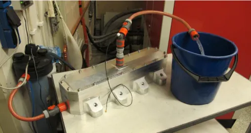
3.6 Filling the rig with water

To fill the rig with water and keep it water tight when filled up, Gardena hose couplings were used. Water was filled through a ball valve coupling attached to the bottom piece which was closed when the rig got completely full. When filling the rig with water, air could escape through couplings in the lid which were divided by a y-coupling. Through one of the outlets a cable connected to the accelerometer on the rod inside comes out, this outlet was plugged with silicon to keep it water tight. The other outlet was fitted with a ball valve coupling with a piece of hose extended above. When the rig was full and there was a water pillar in the hose above the ball valve coupling, it was closed to ensure that the water cavity within the rig was enclosed with a minimum of air inside. To further reduce the risk of a short circuit at the connection between accelerometer and accelerometer cable inside the rig, deionized water was used. Figure 18 shows the procedure of filling the rig with water.

(21)

16

Figure 18. Filling the rig with deionised water before wet vibration tests.

3.7 Vibration test sweeps

All three test specimens were tested in air and in water for sweeps starting at 20 Hz or 100 Hz and going up to 1400 Hz with stepped sine as input. For all materials no notable response was measured before the first rigid body mode which occurred at different frequencies for the different materials and was the reason for starting the sweeps at 20 Hz or 100 Hz. The sweeps were stopped at 1400 Hz because then the first three bending modes were captured in both air and water for all three materials. The sweeps were done at a speed of 0.5 octaves/min which means that each frequency was excited the same number of times but that the sweep progressed faster for higher frequencies.To get good data the electrodynamic shaker was set to regulate and keep the rod at a constant acceleration of 14 m/s2_{RMS which corresponds to about 1 g filtered. To do so the armature had to give low accelerations}

at the eigenfrequencies of the rod and high accelerations at anti resonance or parts of the frequency ranges where the frequency response is low. If instead the armature was set to be kept at a constant acceleration, the acceleration of the rod would be too high at its resonance frequencies and so low at anti resonance that electronic noise in the measurement equipment disturb the data signals. It was shown that for accelerations of about 5 g and above overtones were introduced in the shaker why the armature was limited to a maximum acceleration of 30 m/s2_{. This resulted in frequency ranges where}

the acceleration of the rod could not be kept at 14 m/s2_{but still it was high enough to keep above}

(22)

17

4. Simulation

This part will cover how the solid-acoustic finite element model was set up, what assumptions were made and what simplifications were implemented in the model. All simulations were done in the commercial FEM software Comsol Multiphysics 5.3a.

4.1 Geometry

The geometry that was modelled was only the custom-made rig designed for these tests which was imported to Comsol as a slightly simplified version of the original CAD-model. Simplifications were such as that small and sharp edges were removed to simplify meshing and increase the mesh quality. It was also simplified by not including bolts and boltholes between the three parts of the rig. Most simulations were done for the rig as one solid component but also where the stiffness of the bolts were modelled as thin elastic layers which will be further described later on.

Neither bottom plate nor any part of the electrodynamic shaker was modelled, and the vibrations were applied to the rig through pre-set displacement in the boltholes attaching bottom part to bottom plate. Figure 19 shows the model geometry used in the simulations.

Figure 19. Simplified outer model geometry.

Sliders and hubs to connect springs between rig and rod were not modelled and instead springs were modelled directly between rig and rod which had to be considered when applying spring constant. How this was done and the position of the springs are highlighted in Figure 20.

(23)

18

As was shown in the Impulse hammer tests the relatively small mass and volume of an accelerometer attached at the end of a rod had significant impact on the results, it had to be modelled and included when doing simulations. The mass was measured by putting an accelerometer on a scale and holding the attached accelerometer cable in as close as possible to the same way as it was hanging in the rig. The mass of an accelerometer was 4.6 g and the total mass including cable was 7.5 g. This was a measurement with quite low precision, but running the simulation for a mass of 6.5 g instead of 7.5 g showed that the first bending mode for the aluminium rod in air changed only 2 Hz equal to 0.7 % and in water 1 Hz corresponding to 0.5 %. The added mass from the accelerometer has less influence on the copper rod as it is heavier. First the accelerometer was modelled according to its real geometry as a 10x10x10 mm cube but in the connection between rod and accelerometer the mesh quality did not match up well. Therefore it was instead modelled as a 10 mm cylindrical extension of the rod but with different material properties. This was considered an adequate simplification as the volume was close to the same as well as the projected area in the motion direction and because the added mass had larger influence than the geometry.

4.2 Material

Material properties for aluminium, copper and glass fibre were taken according to what was derived from the Impulse hammer tests. Accelerometer density was applied such as to give a mass of 7.5 g and its Young’s modulus was estimated to 2 GPa which had low impact on the results. Water was modelled with a speed of sound of 1480 m/s and a density of 1002 kg/m3_{corresponding to standard values for}

sweet water. These properties were not measured but running the simulations with 10% lower water density corresponding to 900 kg/m3_{resulted in a change of the first bending mode for the aluminium}

rod of only 1.5 Hz. 10% is an exaggerated error as sea water density typically ranges between 1020 and 1030 kg/ m3_{and still the influence is small. Properties of air were set to a speed of sound of 343 m/s}

and a density of 1.2 kg/m3_.

4.3 Boundary conditions

Simulations were done both with and without modelling the stiffness of the bolt joints connecting the three parts of the rig. Thin elastic layers between contiguous surfaces were used to model the bolts where total stiffness

k

_joint was calculated as a summation of the stiffness of all bolts in each joint.

𝑘

_{𝑗𝑜𝑖𝑛𝑡}

= ∑

𝐸𝐴

𝐿 ( 2 )

E is the Young’s modulus of the bolts, A the load carrying cross section area and L the length of the bolt. The upper bolt joint consisted of 20 stainless M6 bolts with a length of 80 mm while the middle joint consisted of the same 20 bolts and additional 4 M6 bolts with a length of 55 mm. Young’s modulus for stainless steel was taken as 200 GPa and load carrying cross section area as 20.1 mm. For the upper layer the total stiffness became 1.0e9 N/m and for the middle layer 1.3e9 N/m which was divided by and evenly distributed over the connecting surface area between each part of the rig. Where the layers are positioned, and their surface area is shown in Figure 21.

(24)

19

Figure 21. Thin elastic layers to model the two bolt joints.

As mentioned the bottom plate was not modelled and was consequently assumed rigid. The bolt joint between bottom part and bottom plate was modelled with rigid connectors in the boltholes where the surfaces of the boltholes are rigid. Position of the bolt holes are highlighted in Figure 22.

Figure 22. Position of boltholes for connecting the rid to the bottom plate.

It was also in these rigid connectors that vibrational motion from the shaker was introduced and modelled through prescribed vertical displacement amplitude

𝑢

𝑧 as a function of frequency

𝜔.

𝑢

𝑧

= −

1

𝜔2 ( 3 )

For harmonic vibrations with an amplitude expressed as in Equation 3 the displacement as a function of time t is

𝑑𝑖𝑠𝑝𝑙𝑎𝑐𝑒𝑚𝑒𝑛𝑡 = − 1

𝜔2𝑠𝑖𝑛(𝜔𝑡). ( 4 )

By deriving the displacement in Equation 4 twice an expression for time dependant acceleration is acquired described as

𝑎𝑐𝑐𝑒𝑙𝑒𝑟𝑎𝑡𝑖𝑜𝑛 = 𝜔2 1 _𝜔₂𝑠𝑖𝑛(𝜔𝑡) = 𝑠𝑖𝑛(𝜔𝑡).

(

5 ) Equation 4 and 5 shows that with a displacement amplitude of

−

1

𝜔2introduced in the bolt holes, as

shown in Figure 22

,

a constant acceleration amplitude is acquired for the shaker at all frequencies. In the experiments the acceleration of the shaker was regulated to keep a constant acceleration for the rod instead. That was done, as described in 3.7 Vibration test sweeps, to avoid noise at anti resonance and too high accelerations to measure at resonance. As the frequency response function is the ratio between rod and shaker acceleration, that relation will be the same for a constant acceleration on the

(25)

20

rod or on the shaker as long as the sampled data is accurate. Therefore this difference between experiments and simulation does not affect the results.

4.4 Solid-acoustic interaction

The acoustic domain has one degree of freedom which is pressure. On the boundary between acoustic- and solid domains, acoustic pressure causes a fluid load on the solid, and structural accelerations are translated to normal accelerations on the acoustic domain [9].

4.5 Springs

In the test setup of the vibration tests the springs were slightly dispositioned towards the short sides of the rig to give a stiffness component and reduced displacement in the longitudinal direction. In the model this was not considered and simplified by creating springs perpendicular to the surface of the rod. This is not geometrically correct but assuming small deformations it is considered a reasonable simplification. A schematic exaggerated illustration is shown in Figure 23.

Figure 23. Schematic exaggerated view of spring angles in experimental and simulation setup.

Spring constants were measured for the springs used during vibration testing but since sliders and hubs were not geometrically part of the simulation the modelled springs were longer than in reality which is illustrated in Figure 24.

Figure 24. Schematic view of spring connections in experiments and simulations.

Because of the different spring lengths in reality compared to simulations, a new equivalent spring constant had to be calculated for the simulation length. This was done by saying that the same displacement should be acquired for the same force giving the following equation.

𝐹 =

𝑘𝑟𝑒𝑎𝑙 𝜀𝐿𝑟𝑒𝑎𝑙

=

𝑘𝑚𝑜𝑑𝑒𝑙 𝜀𝐿𝑚𝑜𝑑𝑒𝑙

→ 𝑘

𝑚𝑜𝑑𝑒𝑙

= 𝑘

𝑟𝑒𝑎𝑙 𝐿𝑚𝑜𝑑𝑒𝑙 𝐿𝑟𝑒𝑎𝑙 ( 6 )

(26)

21

Where 𝜀 is strain, F is force, k is spring constant and L the spring length

.

It was shown that this spring constant was too stiff as the rigid body modes were too high in the simulations. That was probably because the thin aluminium parts of sliders and hubs where not considered which should lower the stiffness of the complete connection between rig and rod. Which in reality consist of slider, spring and hub but that are modelled with one single spring in the simulation. As this stiffness could not be physically measured and due to quite complicated geometry and bolt connection to the rig it was hard to calculate, a parametric sweep was done in Comsol to find what stiffness gave rigid body modes for the rod that corresponded with the measured ones. There was no spring constant that gave a perfect match for all three materials. Copper required a slightly higher stiffness to match well with measured rigid body modes while glass fibre required a slightly weaker. To get as good an estimate as possible the spring constant giving a good match for aluminium was chosen and used for all materials. This was k = 28000 N/m which was as expected higher than the real measured spring constant k = 21200 N/m, and lower than the one calculated based on increased length but not considering the stiffness of sliders and hubs k = 34600 N/m. Sliders and hubs are stiffer than the springs but weaker than completely rigid.

4.6 Mesh

The rod was meshed with free triangular elements at the end with a maximum element size of 3 mm that was swept along the length with maximum element length of 10 mm as shown in Figure 25.

Figure 25. Detailed view of how the rod was meshed.

The acoustic domain was meshed with free tetrahedral elements and a maximum element size of 35 mm and the test rig was meshed with a maximum element size of 56.7 mm corresponding to the Comsol setting normal mesh size which is related to the overall dimensions of the model. Figure 26 presents a meshed view of the test rig.

(27)

22

4.7 Mesh evaluation and convergence study

To evaluate and show that the mesh used in this study was appropriate, a mesh convergence study was done for the rod and the test rig. When evaluating the mesh of the rod it was isolated and an eigenfrequency study was done for varying mesh sizes using free-free boundary conditions and the material was set to aluminium. Even though the vibration tests were performed up to 1400 Hz and only included the first three bending modes of the test specimens, the ten first eigenfrequencies were calculated and included in the mesh convergence study. The mesh was evaluated for different element lengths along the swept part of the rod varying from 5mm to 150 mm where the one used for all simulations in this report was 10 mm. Figure 27 displays the mesh convergence results acquired for the aluminium rod.

Figure 27. Mesh convergence plot for the aluminium rod including the first ten eigenfrequencies for varying mesh sizes.

Instead of showing the maximum element size on the x-axis in Figure 27 the corresponding number of degrees of freedom is included as that is what actually decides the calculation time. Each curve in the graph corresponds to the n:th eigenfrequency where each dot along a curve is the frequency acquired for each mesh size. The difference between two consecutive points along a curve is how much the eigenfrequency changes for a change in mesh size. Because of the scale of the y-axis the changes are not obvious but what can be seen is that for the coarsest meshes the highest eigenfrequencies differs a lot. That is because when there are only a few elements along the length of the rod it is not possible to describe higher orders bending modes and instead other modes are found. For each bending mode there is one vertical and one horizontal mode that occur at almost the same frequency and therefore only some of them are visible in the graph.

From Figure 27 it can be seen that the results have converged and to confirm that so is the case, a value of convergence C was calculated. It was calculated as the relative difference in eigenfrequency between the mesh size used for all simulations in this report, 10 mm, and a mesh of 20 mm with half the number of degrees of freedom.

0 2000 4000 6000 8000 10000 12000 0 5000 10000 15000 20000 25000 30000 35000 40000 Fre q u en cy [Hz ]

Number of degrees of freedom

Mesh convergence plot for the aluminium rod

Efreq 1 Efre2 Efreq 3 Efreq 4 Efreq 5

(28)

23

𝐶 = (𝜔 10𝑚𝑚−𝜔20𝑚𝑚)

𝜔20𝑚𝑚 ( 7 )

With a maximum mesh size of 10 mm or 20 mm the ten first eigenfrequencies calculated are vertical and horizontal versions of the first five bending modes. Equation 7 was applied for these five bending modes and the different convergence factors are presented in Table 8.

Table 8. Convergence factors C calculated for the first five bending modes of an aluminium test specimen.

Mode C [%] Bending mode 1 0.02 Bending mode 2 0.07 Bending mode 3 0.15 Bending mode 4 0.28 Bending mode 5 0.43

Table 8 shows that all convergence factors up to the fifth bending mode are less than 1 percent which confirms that the mesh used was appropriately fine. For the first three bending modes which are part of the vibration tests the values are much lower than 1 %, indicating that the mesh within the frequency region of interest gives a good representation of the rod stiffness.

The same kind of convergence test was performed for the test rig where the six first

eigenfrequencies were calculated for each mesh size. In this case the different mesh sizes evaluated were the Comsol settings Extremely coarse, Extra coarse, Coarser, Coarse, Normal and Fine which are related to the overall dimensions of the model. For all simulations in this report Normal mesh size was the setting that was used. Figure 28 displays the mesh convergence results acquired for the test rig.

Figure 28. Mesh convergence plot for the test rig including the first six eigenfrequencies for varying mesh sizes.

Figure 28 shows that the results have converged. A relative convergence value C was calculated for the results from a Coarse mesh and a Normal mesh for the first six eigenfrequencies.

𝐶 = (𝜔 𝐶𝑜𝑎𝑟𝑠𝑒−𝜔𝑁𝑜𝑟𝑚𝑎𝑙) 𝜔𝐶𝑜𝑎𝑟𝑠𝑒 ( 8 ) 0 500 1000 1500 2000 2500 3000 3500 4000 4500 0 50000 100000 150000 200000 250000 300000 350000 400000 Fre q u en cy [Hz ]

Number of degrees of freedom

Mesh convergence plot for the test rig

(29)

24

Table 9. Convergence factors C calculated for the first six bending modes of the test rig.

Eigenfrequency C [%] Eigenfrequency 1 0.88 Eigenfrequency 2 0.83 Eigenfrequency 3 1.39 Eigenfrequency 4 0.82 Eigenfrequency 5 0.91 Eigenfrequency 6 0.74

Table 9 shows that the difference between the mesh setting used for the test rig in this report and the next step coarser mesh setting is around one percent which is considered sufficient.

Regarding the mesh of the acoustic domain a common rule of thumb is to choose an element size that gives a resolution corresponding to at least six data points per wave length. In this case the shortest wave length simulated was for 1400 Hz in air and to fulfil the rule in question a maximum element size of 40.8 mm was required and to have some margin 35 mm was chosen. After the meshing was done the maximum element size became 18.6 mm, due to geometric constraints, which gives good resolution for frequencies in air up to 3000 Hz. These calculations show that the mesh is more than satisfactory and therefore no mesh convergence study was performed for the acoustic domain.

4.8 Sweeps

Finally the model was run and evaluated for frequencies ranging from 20 Hz to 1400 Hz with shorter frequency step length close to eigenfrequencies for better resolution and longer in regions where nothing of interest occurred. Solid displacement at a point by the end of the rod where the accelerometer was positioned was evaluated and divided by the input displacement to get the same kind of frequency response function as measured in the vibration tests. In the tests, acceleration was measured but the only difference between displacement and acceleration is the amplitude which cancels out when calculating the ratio of the frequency response. Simulations were run for all three materials in both vacuum, air and water where the rig was modelled as one solid structure. As some behaviours from the test results were not captured in the simulations elastic layers representing the stiffness of the bolt joints were introduced and run for copper in both air and water.

(30)

25

5. Results

From the vibration tests, accelerations were measured for the armature of the shaker, the different parts of the test rig and for one end of the test rod specimens in the frequency domain. With that data it is possible to compare the behaviour between any parts of the rig. The ratio of most interest is between rod and shaker acceleration

𝑎

_𝑟𝑜𝑑and

𝑎

_{𝑠ℎ𝑎𝑘𝑒𝑟}

,

which gives the frequency response function R for each rod described as

𝑅 =

𝑎𝑟𝑜𝑑

𝑎𝑠ℎ𝑎𝑘𝑒𝑟

.

( 9 )

First the results are evaluated with respect to general behaviour and y-axis amplitude R. After that the results are compared to see how well the eigenfrequencies are predicted compared to the experiments where errors are expressed in Hz on the x-axis.

5.1 Problems with test data

When examining the experimental test results, somewhere after the first bending mode they do not look as expected with clear peaks and smooth transitions with lower amplitude in between. Instead there are many large peaks and jagged intervals in between making it hard to determine what peaks correspond to second and third bending mode. Figure 29 shows experimental- and simulation data for all three materials in air plotted in two separate graphs. The simulation data looks like what was expected as well as the first part of the experimental data.

Figure 29. Experimental- and simulation data for all three materials in air.

What can be noted in the experimental data is that after the first bending modes, at about 200 Hz for copper and 250 Hz for aluminium and glass fibre, there are some smaller irregularities and after about 600 Hz and up until the end at 1400 Hz there are regions with large close laying peaks. Some of those behaviours are similar for all three materials which may indicate that they are results of resonance in the rig, which in turn affects the vibrations and accelerations of the rod. In the simulations where the rig is modelled as one solid piece there is no resonance in the rig for the evaluated frequency range. To further evaluate the hypothesis of resonance in the rig, thin elastic layers were implemented in the simulation model between each part of the rig so that they can move in relation to each other. Each layer was given the same total stiffness as the bolts of the bolt joints connecting them. That way some of the unexpected and irregular behaviours shown in Figure 29 above appeared also in the simulation data, see 7.2 Appendix 2, which indicates that the hypothesis is correct. Most likely there is resonance in the bottom plate within the evaluated frequency interval. Possibly also between rig and bottom

(31)

26

plate and between bottom plate and shaker but since those parts were not modelled such behaviours could not be reproduced. Up to about 450 Hz there is no obvious influence from the rig on the results and it is only in this region that it is possible to draw definite conclusions from this study.

5.2 Frequency response function

The results in Figure 30 were acquired for the copper rod in air and are first evaluated with respect to general behaviour and how well the amplitude of frequency response functions correspond.

Figure 30. Frequency response functions for copper rod in air based on experiment and simulation data.

The first region of peaks should consist of one rotational rigid body mode and one translational which are situated close to each other. This is what is given by simulations while the test data in this region is messy with a couple of close laying peaks. This might be due to that there is almost no damping in the system and that vibrations from one eigenfrequency does not have time to die out before excited by a new one and therefore interact with each other. The control system of the shaker was set to keep the rod acceleration constant and in this region it could not do so properly for the reasons just explained. It should also be mentioned that there are two sets of every mode, one in the vertical direction which was measured, and also one in the horizontal direction. In reality it is not possible to acquire perfect symmetry for springs and attachments and as shown when measuring spring length and spring constants there is some small variation. This may lead to acceleration components in both horizontal and vertical direction for respective mode. With almost no damping in air this might also have disturbed the data in this region.

The second peak corresponds to the first bending mode and in both cases amplitude and position are matching well with a small difference in frequency. Exact amplitudes at eigenfrequencies may vary depending on experimental and simulation sample resolution. In the simulations for example the sample resolution was 1 Hz close to the eigenfrequencies but the actual eigenfrequencies are most likely somewhere in between the evaluated frequencies. It should also be noted that in the simulations there is no damping present and all deformations are assumed small which might not be true at eigenfrequencies. Therefore the amplitude at eigenfrequencies differs more between experimental and simulation data than for other regions and that the results are matching as well as they are is promising. Up until the first bending mode, the curves are almost overlapping and after that the general behaviour is the same but with some difference in amplitude.

(32)

27

Figure 31. Frequency response functions for copper rod in water based on experiment and simulation data.

Figure 31 shows the results acquired for the copper rod in water. In water there is more damping which results in two clear peaks for rotational and translational rigid body modes. Again up to about the first bending mode the curves almost overlap and afterwards the general trend is captured with some difference in amplitude. On both sides of the first bending mode and at about 400 Hz there are behaviours in the test data that were not present in the simulation data. What those behaviour corresponds to is hard to say.

Figure 32. Frequency response functions for aluminium rod in air based on experiment and simulation data.

For the aluminium rod results were acquired in air according to Figure 32. The translational and rotational rigid body modes are more separated than for the copper rod which results in a wider region of unstable results. This is probably due to the same reason as explained for the copper rod. Up until the first rigid body mode the two curves correspond well and after that there are some smaller uneven behaviours not captured but the general behaviour is the same.

(33)

28

Figure 33. Frequency response functions for aluminium rod in water based on experiment and simulation data.

Figure 33 shows the results acquired for the aluminium rod in water. The same as for the copper rod in water there are behaviours on both sides of the first bending mode for aluminium in water that were not captured in the simulations. Other than that, the general trend and amplitude correspond well, especially in-between peaks.

Figure 34. Frequency response functions for glass fibre rod in air based on experiment and simulation data.

For the glass fibre rod results were acquired in air according to Figure 34. There is a clear peak for the translational rigid body mode while the data around the rotational rigid body mode became unstable. Otherwise the general trend corresponds well with good correlation in amplitude up to the first bending mode and a slightly increasing difference afterwards. The most notable difference is the difference in amplitude at anti resonance.

(34)

29

Figure 35. Frequency response functions for glass fibre rod in water based on experiment and simulation data.

In water the result shown in Figure 35 was acquired for the glass fibre rod. Overall, the general behaviour is the same between experiments and simulation, but it is for the glass fibre rod in water that the largest differences in amplitude occur. This might be due to a quite rough approximation of modelling glass fibre as an isotropic material where the bending stiffness measured in impulse hammer tests was applied for tension stiffness, compression stiffness and shear stiffness. For composite materials in general this is not the case and still the results correspond quite well. It was also for glass fibre in water that the most surprising test results occurred, namely that there was no peak for the first bending mode. One possible explanation could be that glass fibre has a high internal damping which was not implemented in the model. Unfortunately the transient results from the impulse hammer tests were not saved, otherwise damping coefficients could have been measured and implemented.

5.3 Prediction of eigenfrequencies

Next part of the evaluation is to see how well eigenfrequencies could be predicted using solid-acoustic simulation. That is done by first calculating absolute errors as

𝛿𝑎𝑏𝑠𝑜𝑙𝑢𝑡𝑒= 𝜔0,𝑒𝑥𝑝𝑒𝑟𝑖𝑚𝑒𝑛𝑡𝑎𝑙− 𝜔0,𝑠𝑖𝑚𝑢𝑙𝑎𝑡𝑖𝑜𝑛 [𝐻𝑧]

.

( 10 )

Where

𝛿

is the error and

𝜔

₀

is

eigenfrequency, and then calculating the relative error as

𝛿

_{𝑟𝑒𝑙𝑎𝑡𝑖𝑣𝑒}

=

𝛿𝑎𝑏𝑠𝑜𝑙𝑢𝑡𝑒

𝜔0,𝑒𝑥𝑝𝑒𝑟𝑖𝑚𝑒𝑛𝑡𝑎𝑙

.

( 11 )

As shown and mentioned, experimental data in air around translational and rotational rigid body modes do not present two clear peaks and it is therefore hard to determine which peaks corresponds to the actual eigenfrequencies. To get a comparable value an average of the most outlying peaks of the experimental data is calculated and compared with the average of the simulation peaks for translational and rotational rigid body modes in air. Figure 36 shows how these values are chosen illustrated by magnified views of rigid body modes for the aluminium rod in air. Both graphs are the same but shown twice as the value markers hide some of the data.

(35)

30

Figure 36. Example of data extraction for rigid body modes in air.

Due to increased damping there are two distinct peaks for translational and rotational rigid body modes for all three materials in water. In those cases, it is obvious what values to extract which is demonstrated in Figure 37 with magnified views of rigid body modes for the aluminium rod in water.

Figure 37. Example of data extraction for rigid body modes in water.

What values to extract for the first bending mode in both air and in water is also obvious as there are clear peaks in all cases except for glass fibre in water where there is no peak at all.

Following described procedure, experimental and simulation data can be extracted for rigid body modes and first bending mode for all three materials and absolute and relative errors calculated. By doing so the results in Table 10, Table 11 and Table 12 are acquired.

(36)

31

Table 10. Eigenfrequency data for copper rod in air and in water.

Copper Experiment [Hz] Simulation [Hz] Absolute error [Hz] Relative error [%]

Rigid body modes in air 81.1 77 4.1 5.1

Translational rigid body mode in water 70.1 70 -0.1 -0.1

Rotational rigid body mode in water 74.6 75 0.4 0.5

First bending mode in air 193.9 189 4.9 2.5

First bending mode in water 182.2 179 -3.2 -1.8

Table 11. Eigenfrequency data for aluminium rod in air and in water.

Aluminium Experiment [Hz] Simulation [Hz] Absolute error [Hz] Relative error [%]

Avg. of rigid body modes in air 130.1 133.5 3.4 2.7

Translational rigid body mode in water 105.3 108 2.7 2.6

Rotational rigid body mode in water 117.3 123 5.7 4.9

First bending mode in air 245.7 241 -4.7 -1.9

First bending mode in water 209.8 211 1.2 0.6

Table 12. Eigenfrequency data for glass fibre rod in air and in water.

Glass fibre Experiment [Hz] Simulation [Hz] Absolute error [Hz] Relative error [%]

Avg. of rigid body modes in air 145.3 147.5 2.2 1.5

Translational rigid body mode in water 109.8 114.0 4.2 3.8

Rotational rigid body mode in water 126.4 133.0 6.6 5.2

First bending mode in air 238.7 236.0 -2.7 -1.1

First bending mode in water - 198.0 - -

The largest relative errors in prediction of eigenfrequencies for each respective material occurred for the rigid body modes while the first bending mode was predicted with very good accuracy in all cases. That is not surprising as the rigid body modes depend on the stiffness of the spring connections between rod and rig which could not be measured and were approximated as previously described. The largest relative error for the rigid body modes was 5.2 % and only 2.5 % for the first bending modes.

(37)

32

6. Discussion and Conclusions

This study consists of an experimental and simulation based comparison for water submerged rods suspended within a cavity with close laying boundaries excited by forced vibration. The comparison was made to investigate how accurately this intricate fluid structure interaction problem can be modelled with water as an acoustic medium, and that with respect to prediction of eigenfrequencies and frequency response function up to 1400 Hz. Rods with the same dimensions made of copper, aluminium and glass fibre are evaluated.

The results of this study show good accuracy in prediction of rigid body modes and first bending mode. For all three materials the maximum error for the rigid body modes was 5.2 % and 2.5 % for the first bending modes. Frequency response functions are predicted capturing the general behaviour with reasonable accuracy in amplitude up to 450 Hz. At higher frequencies the data could not be properly evaluated because of noise probably due to resonance in the test rig interfering with the behaviour of the rod specimens.

Though no conclusions can be drawn for higher frequencies it is believed that this simulation method should be applicable there as well. The copper rod which has the lowest specific stiffness of the three test specimens and therefore the most easily excited rod, shows good correlation for second and third bending mode with peaks in the test data. It is not possible to prove if the corresponding peaks in the test data are due to resonance of the rod or not, but it is likely.

Resonance in the rig was the largest problem that was encountered as it restricted the conclusions that could be drawn from this study and therefore only part of the aim could be fulfilled. There are two main ways that this problem could be dealt with in continued studies. Either the simulation model could be improved to better represent reality and see how well resonance in the rod as well as the rig could be captured. For one thing the whole system has shown to be rather complex and hard to model properly and still if there are differences it would be hard to interoperate the frequency response function and determine what peaks correspond to what resonance. Another approach would be to make a stiffer test rig with increased wall thicknesses and especially more and thicker bolts in each bolt joint. That way eigenfrequencies of the rig could hopefully be increased above 1400 Hz and if not, at least the amplitudes would be reduced with less disturbance of the rod measurements.

With respect to prediction of the rigid body frequencies no strong conclusions can be drawn. That is because they depend on the stiffness of the spring connections between rig and rod which cannot be physically measured and therefore approximated as previously described. But, since the general behaviour of the frequency response function was captured for the rigid body modes and the bending modes were predicted with good accuracy, it is reasonable to believe that the model is equally accurate in predicting rigid body modes.

Related to the aim and hypothesis of this study the conclusions that can be drawn are that at least up to 450 Hz eigenfrequencies can be predicted with good accuracy and that general behaviour of frequency response functions could be captured in air and water. For real world applications of submerged structures where deformations are small and added mass effects of water are dominant, the accuracy shown in prediction of frequency response is high enough for design purposes. It is also a fast method possible to be implemented in early stages of design, allowing for optimisation and evaluation of different underwater design concepts. This is something that with other available methods has not been possible before.

Experimental and numerical fluid-structure interaction analysis of a suspended rod subjected to forced vibrations

Kungliga Tekniska Högskolan

Master thesis