The Ganges drainage basin: Hydrological transitions due to anthropogenic water use.

TRITA-LWR Degree Project ISSN 1651-064X

LWR-EX-2014:20

T

HE

G

ANGES DRAINAGE BASIN

:

H

YDROLOGICAL TRANSITIONS DUE TO

ANTHROPOGENIC WATER USE

Tushar Agarwal

Tushar Agarwal TRITA-LWR Degree Project 14:20

ii © Tushar Agarwal 2014

Degree Project Environmental Engineering and Sustainable Infrastructure Done in association with the Water Resources Engineering Research group Division of Land and Water Resources Engineering

Royal Institute of Technology (KTH) SE-100 44 STOCKHOLM, Sweden

References should be written as: Agarwal, T. (2014) "The Ganges drainage basin: Hydrological transitions due to anthropogenic water use" TRITA-LWR Degree Project 14:20.

iii

D

To Satyajit Ghosh,

Thank you for inspiring me into research. Quoting Gandhi, “Be the change you wish to see”, I hope this work would bring a new dimension of thought towards the Ganges basin.

Tushar Agarwal TRITA-LWR Degree Project 14:20

v

S

S

Gangesflodens avrinningsområde är ett av världens största färskvattenförråd. Området är ca 1 million kvadratkilometer stort och befolkas av mer än en halv miljard människor. Hydrologiska undersökningar av området är dock få och innefattar inte förändringar av mänsklig vattenanvändning och dess effekter över tid på vattnets kretslopp i regionen. Dock har många studier undersökt hur förändringar i land- och vattenanvändning i avrinningsområden i andra delar av världen kan påverka den lokala hydrologin. Gangesområdet har upplevt en snabb utbyggnad av konstbevattningssystem sedan 1960-talet för att mätta matefterfrågan hos en växande befolkning. Konstbevattnat jordbruk har ökat från 18 till 48 % mellan 1962 och 2003. Den här studien är framförallt fokuserad på att förstå konstbevattningens roll i avrinningsområdets vattenbalans. Hydrologisk modellering av Gangesflodens avrinningsområde gjordes i PCRaster med en vattenflödesmodul av POLFLOW. För analysen användes följande data: DEM, vattendrag, nederbörd, temperatur, ytvattenanvändning, grundvattenanvändning, area med konstbevattning (både från grund- och ytvatten) och uppmätt vattenflöde vid Gangesflodens mynning. Konstbevattning användes i modellen genom addering till nederbörden. Tre olika scenarior användes för analysen: ett för perioden före utbredd konstbevattning (1951-1959), ett med konstbevattning (1991-2000) och ett med ett hypotetiskt klimat för 1991-2000. Modellen kalibrerades med hjälp av det observerade utflödet i scenarierna utan konstbevattning (1951-1959) och med konstbevattning (1991-2000). Mellan dessa två perioder minskade nederbörden med 129 kubikkilometer per år och evapotranspirationen minskade ännu mer. Å andra sidan minskade även utflödet med 18.41% på samma tid. Dessutom visar modellens resultat en ökning av kvoten mellan evapotranspiration och nederbörd från 0.483 till 0.525. Den stora skillnaden mellan minskningen i nederbörd och evapotranspiration kan antagligen tillskrivas vattenanvändningen för konstbevattning. Dessutom kan konstbevattning vara en viktig orsak till minskad vattentillgång nedströms i avrinningsområdet på grund av den ökade kvoten mellan evapotranspiration och nederbörd under konstbevattningsscenariet. Yt- och grundvatten för konstbevattning bidrar till ökad evapotranspiration och minskar därmed utflödet från Gangesfloden. Minskad vattentillgång nedströms begränsar och förhindrar vattenanvändning, framförallt under torrperioder. Den geografiska förändringen av evapotranspirationen över tid kan vara ett allvarligt bekymmer ur ett klimatperspektiv. Med mer än en halv miljard av jordens befolkning direkt eller indirekt beroende av Gangesflodens avrinningsområde för sin försörjning är det en ren nödvändighet att implementera mer effektiva bevattningstekniker och planera för en integrerad vattenhushållning för att klara en växande befolkning. Den här studien kan erbjuda en grund för att undersöka sambandet mellan klimat och konstbevattning i regionen.

Tushar Agarwal TRITA-LWR Degree Project 14:20

vii

A

This work would be incomplete without thanking my Supervisor/ Examiner Vladimir Cvetkovik for his continuous moral and financial support, my parents for letting me follow my heart, my brother for always standing as a pillar in times of need and Sat Ghosh for preparing me for a Master’s in Sweden. In addition, I appreciate and thank my friends at KTH- Xenofon LBR for encouraging me to learn ArcGIS and helping me to edit my thesis; Guillaume Vigouroux for bailing me out of troubled waters every time; Xavier Mir for assisting me in learning PCRaster and Otto Rimfors for helping me with the Swedish translation. Working in the same cabin for almost 6 months would not have been so fun without the effervescent presence of Mengni Dong who would have us in splits so many times. I would also like to acknowledge Sofie Soltani for integrating me in the assigned cabin and Aira Saralainen for providing a smooth sail in the concerned matters. Last but not the least; I appreciate the constructive comments received from Lea Levi and Robert Earon to improve my thesis.

Tushar Agarwal TRITA-LWR Degree Project 14:20

ix

T

C

Results and discussions ... 4

Conclusions ... 9

Limitations ... 9

References ... 10

Tushar Agarwal TRITA-LWR Degree Project 14:20

xi

A

GDB: Ganges drainage basin P: Precipitation

ET: Evapotranspiration R: Runoff

T: Temperature

Tushar Agarwal TRITA-LWR Degree Project 14:20

1

A

Hydrological changes in catchments world over have affected regional climate and pose serious challenge to future water resource management. The Ganges drainage basin (GDB) is one such region which has undergone rapid transformation in land and water use, more specifically in the latter half of 20th _century.

GDB has a population of more than half a billion people and is spread across India, China (Tibet), Nepal and Bangladesh. Further, hydrological investigations accounting land and water use changes in GDB are rare. This study is an attempt to resolve hydrological changes in the Ganges basin using the fundamental water balance, focusing particularly on water use changes through irrigation. Between the period 1951-1959 and 1991- 2000, precipitation (P) in the Ganges basin has reduced by 11.25 % while evapotranspiration (ET) has only reduced by 3.61 %. In addition, the ET/P has increased from 0.483 to 0.525 during the same period suggesting a larger partitioning of P towards ET. This suggests greater utilization of P to release water vapor in the atmosphere and thus causing a reduced water flow downstream. With water availability at the fulcrum of future concern for regional and national water security, these findings should encourage policy makers to account for hydrological changes in the GDB in planning sustainable water use.

Key words: Irrigation; Precipitation; Evapotranspiration.

I

Recent studies have shown the impact of irrigation on water cycle and local- regional climate (Boucher et al, 2004; Lobell et al, 2009; Jarsjö et al, 2012; Huber et al, 2014). There have been instances of reduced runoff (R), increased

evapotranspiration (ET) and changes in

atmospheric and surface conditions (temperature,

humidity, cloud formation, radiation and

precipitation) due to imposed changes on land and water use (Asokan et al, 2010; Destouni et al, 2010; Jarsjö et al, 2012; Dadson et al, 2013; Harding et al, 2013). In the global context, irrigation has increased ET by approximately 2600 km3_{/year which constitutes a large portion of}

freshwater use (Gordon et al, 2005). Other drivers known to have significantly impacted ET are deforestation, hydropower development and non- irrigated agriculture (Gordon et al, 2005; Destouni et al, 2013). Indications are rife that increasing ET in one region due to growing food production could impact the capability of other regions to satisfy their food requirements (Gordon et al, 2005). One region which has been at the forefront of rapid irrigation expansion is the Ganges drainage basin (GDB), majority of which lies in India.

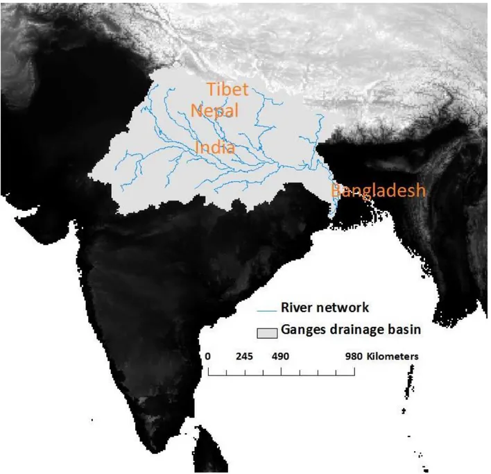
The Ganges river system originates in the Central Himalayas, extends into the alluvial plains of Ganges and drains into the Indian Ocean at the Bay of Bengal. Figure 1 shows the extent of GDB. Its basin area (1.08 million km2_{) spreads across}

four countries namely India (79 %), Nepal (13 %),

Bangladesh (4 %) and Tibet (China) (4 %) (Bharati et al, 2011). With a total population of approximately 600 million people (Rajmohan and Prathapar, 2013) and a population density of 550 persons/ km2 _{(Jain et al, 2009), it is one of the}

most populous river basins in the world.

Along GDB, R is influenced not only by snow and ice-melt but also by fluctuating monsoonal precipitation (P). However, the contribution of snow and ice melt to the total R of the GDB is minimal and is estimated to be between 1-5 % of annual basin R (Moors and Siderius, 2012). Hence, a major portion of R from GDB comprises of the monsoonal P. These monsoons occur in two periods- south- west monsoon and north- east monsoon. South- west monsoon starts from June and end in September. It contributes majority of P in GDB. North- east monsoon, also known as retreating monsoon occurs during the period September- December and provides low P in the Ganges belt.

There are mainly two sources of irrigation in the GDB- (i) surface water diverted through channels into agricultural land and (ii) groundwater extraction. Over the years, the role of groundwater irrigation has considerably increased in the basin. Regarded as the `bread basket' of South Asia (Moors et al, 2011), the region is intensely irrigated and is under severe stress to address food requirements of a rapidly growing population (Aggarwal et al, 2004; Gordon et al, 2005; Siebert et al, 2005; Harding et al, 2013). The aim of this study is to investigate the temporal change in water balance in the GDB in

TusharAgarwal TRITA-LWR Degree Project 14:20

2

Figure 1. Extent of GDB along with Ganges river network.

the latter half of 20th _{century by comparing two}

different water use scenarios- preirrigation (1951-1959) and irrigation (1991-2000). In addition a hypothetical climate scenario is invoked to evaluate changes in water balance due to a climate transition. Furthermore, a spatial analysis is also performed for selected components affecting the water availability in the basin.

M

The following datasets were used for the hydrological analysis of the GDB- DEM, water

lines data, P data, temperature (T) data, surface water use data, groundwater use data, area under irrigation data (surface as well as groundwater) and observed R at the outlet. DEM and water lines data were obtained at a spatial resolution of 0.008 decimal degrees (DIVA- GIS, 2014). Monthly T and P data for the GDB was obtained from the Climate Research Unit database CGIAR-CSI CRU-TS v3.10.01 for the years 1991-2009 at 0.5 degree spatial resolution (Jones and Harris, 2013). Global maps of areas irrigated with groundwater and surface water were acquired at a spatial resolution of 0.08 decimal degrees (Siebert et al,

3 2013). Observed R was collected for the period

1951- 2000 (Eastham et al, 2010). Irrigation water use from surface and groundwater reserves was also acquired (World Bank, 2011). Groundwater use during the period 1991- 2002 was determined from temporal estimates of groundwater irrigation in Indian parts of GDB (Bhaduri et al, 2006). Irrigation is known to exist for centuries in GDB; however, significant growth has occurred after 1960’s. Particularly in the Indian parts of the basin, irrigated agriculture has increased from 18 % in 1962 to 48 % in 2003 (Bhalla and Singh, 2010). In addition, cultivated area and rainfed cultivation have also increased during the same time. While groundwater use for irrigation has been a more recent development which coincides with the advent of green revolution of late 1960’s in India, surface water has its roots back to around 14th _{century. There is, however, a surge in the use}

of surface water for irrigation since the 1960's. An estimated 112 km3_{/ year of water is used from}

surface sources in India. Approximately, 88 km3_/

year has been diverted since the 1960's (World Bank, 2011). Some of the routing was completed around the year 2000. However, their construction had started long before and water extraction was quite likely happening. In case of groundwater, approximately 94 km3_{/ year of water is extracted}

for irrigation in India (Bhaduri et al, 2006; World Bank, 2011). In total, 206 km3 _{of water is used}

annually for irrigation. These extractions could still be an underestimation of water actually withdrawn from surface and subsurface. An approximate 375 km3_{/ year of water is estimated}

to be used for irrigation in the Ganges basin, of which more than 50 % is groundwater (Moors and Siderius, 2012). However, these estimates are as recent as 2008 and do not demarcate spatial use of surface and groundwater extraction in GDB. The ‘preirrigation scenario’ is defined as the period (1951- 1959) during which irrigation water use was fairly constant at around 18 % of the total water used for cultivation. In addition, the availability of R data from 1951 onwards allows model calibration for this period. The period 1991- 2000 is chosen as the ‘irrigation scenario’ due to large expansion of irrigation and a declining R (Figure 2). An additional ‘climate scenario’ was hypothesized to analyze the hydrological change only due to P and T transition from 1951-1959 to 1991- 2000. In this particular scenario, irrigation activity over the Ganges basin was not considered.

In the first step, all raster data were resampled to a spatial resolution of 0.08 decimal degrees. GDB was delineated using tools present in Arc Hydro extension of Arc Map 10. This required the use of DEM and water line data. After developing the catchment area of Ganges along with the river network, climate data (T and P) was processed for GDB in ArcGIS. Spatial maps of mean annual T and P were generated for both the periods- 1951- 1959 and 1991- 2000. This was followed by the spatial distribution of surface and groundwater in the catchment for the irrigation scenario. To develop these maps, total water used for irrigation

from surface (112 km3_{) and groundwater reserves}

(94 km3_{) was spread uniformly over the areas}

equipped with surface and groundwater irrigation based on their fraction of grid cell under irrigation. In the irrigation scenario, water used as irrigation was added as extra P.

The hydrological modeling of GDB was performed on PCRaster using water flow module of the code POLFLOW (De-Wit, 2001). It had been adopted for hydrological modeling of catchments such as Mahanadi River Basin in India (Asokan et al, 2010) and Aral Sea Drainage Basin in Central Asia (Jarsjö et al, 2012). PCRaster is a set of spatio- temporal functions which can be embedded in a programming language such as Python to modify, model or create raster maps. The raster maps can be displayed using PCRaster function ‘aguila’ or can be exported to ArcGIS. The number of functions which can be used in PCRaster are limited in comparison to ArcGIS and may require the use of another software for pre-processing or post-processing of data. However, the strength of PCRaster lies in the easy programming of environmental processes which is quick and flexible when compared to step by step operations in ArcGIS. The following paragraph provides the description of POLFLOW module used in PCRaster.

The hydrological analysis of the GDB was performed using the basic water balance quantification shown in equation (1). In this analysis, the change in water storage in GDB is assumed, ΔS≈0 for simplifying the calculations. Also the lack of data restricts the use of storage term and limits the scope of work as there are certain parts which have witnessed a drop in water level. The ET consists of evaporation from surface and subsurface water and transpiration

TusharAgarwal TRITA-LWR Degree Project 14:20

4 from plants. It is suggested that the ET errors

which arise from the principal basin scale water balance closure are below 20% (Asokan et al, 2010). On the other hand, error in the ET estimates from Penman- Monteith model equations can vary between 30-55 % when they are not calibrated from runoff observations (Kite and Droogers, 2000).

� − � − − ∆ = (1) P: precipitation (mm/year)

ET: evapotranspiration (mm/year) R: river runoff (mm/year)

ΔS: water storage change (mm/year)

Spatial distribution of actual ET was calculated in two steps- first potential ET for each grid cell in GDB was computed using empirical method (Langbein, 1949) as shown in equation (2):

� = 5 + ∗ + .9 ∗ 2 ₍₂₎

Ep: potential ET (mm/year)

T: mean annual temperature (o_C)

Secondly, using Ep and mean annual P, modeled

ET was estimated for each grid cell in the GDB from the following equation (Turc, 1954):

� � � = �

√0.9+ �2_/� 2(3)

ETmod: modeled ET (mm/year)

In addition, total modeled ET for the GDB was calculated by adding ETmod for each cell. Using

equation (1), modeled R (Rmod) was calculated for

the basin in the unit of km3_{/year. The ET in}

equation (3) is empirical and thus requires calibration. As there are no recorded historical measurements of ET, its calibration was performed by balancing the modeled R with observed R (Robs) over a given period. Firstly, an

assumption was made that the actual ET is a product of ETmod and a calibration factor (Jarsjö

et al, 2008) as can be seen in equation (4):

�� = � ∗ � � �(4)

AET: actual ET (mm/year) X: calibration factor

X will be equal to 1 if AET= ETmod. X was

calculated using Robs, Rmod, P and ETmod (Jarsjö et

al, 2012) and can be seen in equation (5):

� = � �� �� �+ − � �� �� � ∗ ∑ � ∑ ��_{� �}(5) ΣP= total P (km3_/year)

ΣETmod= total modeled ET (km3/year)

All terms in equation (5) are in the unit km3_/year.

R

Figure 2 shows 10 year running mean of P, T and R. As can be observed, P increases in the first half of 20th _{century, reaches a maximum of 1178 mm}

in the year 1946 and then starts declining to record its lowest value of around 950 mm in 1997. In case of T, there have been more fluctuations leading to an increase in first half of 20th _century,

then a decline till mid 1970’s and later an increase towards the end of 20th _{century. In addition, the}

10 year running mean shows a rise in recorded T from 19.8 to 20.4 o_{C between 1905 and 1997. R,}

on the other hand has fluctuated- initially it increased and then decreased for a short span, followed by some stability towards a higher value and eventually falling down to its lowest record in latter half of 20th _century.

The spatial variation of mean annual P during the 1991- 2000 can be seen in Figure 3. P is lower in the western and northern parts while higher in the central, southern and eastern parts of the basin. Furthermore, the spatial change in mean annual P between the periods 1991- 2000 and 1951- 1959 is displayed in Figure 4 which is the difference between more recently recorded P (1991-2000) and earlier records of P (1951-1959). P has reduced in most parts of the basin. While areas of P increase are few and are generally in proximity of the basin boundary.

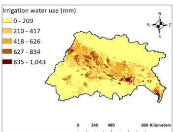
Spatial distribution of mean annual T for the period 1991- 2000 is shown in Figure 5. Generally, northern region of GDB records lower T when compared to other parts of the basin- south, south- east and south- west. Figure 6 illustrates the change in T between 1991- 2000 and 1951- 1959 time periods. Except for T decrease in some upstream regions, rest of the GDB has warmed. Irrigation water use from ground and surface extractions is demonstrated in Figure 7. A noticeable trend is that areas of intense irrigation occur near the main stem of Ganges river system, as these would be the most fertile regions.

5

Figure 2. 10 year running mean of P, R and T in the GDB.

It can also be seen that irrigation is widespread in the GDB with some areas using as high as 1000 mm of water per year. These extractions are comparable to the mean annual P in this region. The availability of runoff observations for the period 1951- 2000 allowed the calibration of hydrological model for the preirrigation and irrigation scenarios. In the preirrigation scenario, Robs= 592 km3/year, Rmod= 329.25 km3/year,

∑P= 1146 km3/year and ∑ET_{mod= 816.7}

km3_{/year. Using equation (5), the calibration}

factor was determined to be X= 0.68. For the irrigation scenario, the calibration factor was calculated X= 0.62 when Robs= 483 km3/year,

Rmod= 153.4 km3/year, ∑P= 1017 km3/year and

∑ETmod= 863.5 km3/year. While in case of the

hypothetical climate scenario, calibration cannot be performed since observed runoff is not available. However, to achieve a more realistic representation of climate scenario, calibration factor of preirrigation scenario is assumed. This assumption can be disputed but the basis is to scale the ET and R to the prevailing conditions

which as per the calculations above indicate calibration factor in the range 0.6-0.7.

Table 1 summarizes the average temperature and water flows in the GDB for all three scenarios. In addition it also shows the percentage change in different parameters from preirrigation to irrigation scenario.

Figure 3. Spatial variation of mean annual P for the time period 1991- 2000 (in mm/ year).

TusharAgarwal TRITA-LWR Degree Project 14:20

6

Figure 4. Spatial variation of change in mean annual P between 1991- 2000 and 1951- 1959 time periods.

Figure 5. Spatial variation of mean annual T for the time period 1991- 2000.

Figure 6. Spatial variation of change in mean annual T between 1991- 2000 and 1951- 1959.

Water flows comprise of total P, total modeled ET, modeled R at outlet along with water used for irrigation (groundwater and surface water) in km3_/

year.

Figure 7. Spatial distribution of irrigation water use in GDB (in mm/ year).

Between the periods 1951- 1959 (preirrigation) and 1991- 2000 (irrigation), mean T has increased by 0.023o_{C with a 0.114 % increase. During the}

same period, P has decreased by 129 km3_{/ year}

(11.25 %) while ET has reduced by 20 km3_{/ year}

(3.61%). In comparison to P decrease, ET drop is much lower. On the other hand R has reduced by 18.41 %. Another important criterion to analyze the effect of irrigation on ET is ET/P fraction which quantifies evapotranspiration per unit precipitation during each scenario. For the preirrigation and climate scenario, ET/P is calculated as 0.483 and 0.51 respectively. On the other hand ET/P for irrigation scenario is 0.525. It is difficult to rely on ET/P for climate scenario due to its hypothetical nature and lack of observed runoff records. ET/P for irrigation scenario is higher than the ET/P in preirrigation scenario (8.69 %). This means that ET has increased per unit P in the basin.

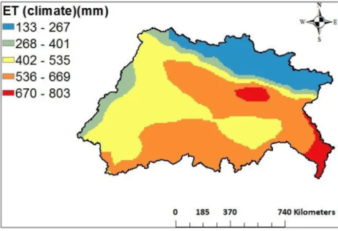
The spatial distribution of ET for different scenarios can be seen in Figure 8, Figure 9 and Figure 10. In case of preirrigation scenario (Figure 8), large ET flows are found in most parts of the basin, except the northern and western regions. The highest ET is concentrated in the eastern and central parts. On the other hand, ET has become higher in some of the western parts and decreased in south and south- western regions in case of irrigation scenario (Figure 9).

7

Table 1. Summary of T and water flows in GDB.

Also highest ET has spread across the center of the basin. It can also be noticed that except the northern regions, ET has redistributed in most of the GDB. In climate scenario (Figure 10), there are more areas showing lower ET when compared to preirrigation and irrigation scenario.

This can be attributed to lower P in case of climate scenario (1991- 2000) when compared to preirrigation scenario (higher P) and irrigation scenario (extra P added as water for irrigation). Figure 11 displays the percent change in ET

Figure 8. Spatial distribution of annual ET in preirrigation scenario (1951- 1959).

during the transition from preirrigation to irrigation scenario represented as the difference between irrigation and preirrigation scenario. It can be observed that ET has decreased in more parts when compared to regions with ET increase. The highest drop in ET which is around 24 % extends along a diagonal from north- west to south- east and in some southern parts as well. On the other hand, ET has increased by more than 50 % in some western parts. Also, higher ET

Figure 9. Spatial distribution of annual ET in irrigation scenario (1991- 2000). Variables Preirrigation scenario (1951-1959) Climate scenario (1991-2000) Irrigation scenario (1991-2000) % Change from preirrrigation to irrigation scenario Temperature (oC) 20.225 20.248 20.248 0.114 Precipitation (km3/year) 1146 1017 1017 -11.25 Groundwater use (km3/year) 0 0 94

Surface water use

(km3/year) 0 0 112 ET (km3/year) 554 520 534 -3.61 Modeled Runoff(km3/year) 592 497 483 -18.41 Observed Runoff (km3/year) 592 483 ET/P 0.483 0.511 0.525 8.69

TusharAgarwal TRITA-LWR Degree Project 14:20

8

Figure 10.Spatial distribution of ET in climate scenario.

loss can be noticed near the basin outlet which is situated in south-east.

The percent change in ET between preirrigation and climate scenario represented as the difference between climate and preirrigation scenario, is illustrated in Figure 12. ET drop is evident in most parts of the basin due to lower P during 1991- 2000. In particular, downstream parts of the basin show maximum decrease in ET. There are also some areas which show increased ET and are geographically located at the edge of basin. The maximum increase in ET in these areas is not more than 17 %, which is mainly attributed to a higher local P in comparison to 1951- 1959. The difference between Potential ET (PET) and ET for all the scenarios is elucidated in Figure 13, Figure 14 and Figure 15.

Figure 11. Spatial distribution of ET change between irrigation and preirrigation scenario (in %).

Figure 12.Spatial distribution of ET change between climate and preirrigation scenario (in %).

The difference is highest in climate, followed by preirrigation and then lowest in irrigation scenario, particularly in irrigated regions (north- west, central and south- east).

While ET represents the supply side of water vapor to atmosphere, PET is the measure of atmospheric moisture demand. Their difference signifies how much more water can the atmosphere hold in a given scenario. Mostly related to water resource management, it is a measure of crop water need to achieve maximum productivity (Pidwirny, 2006). The crop water need seems to be lowest in preirrigation scenario even though the irrigation scenario looks very much similar.

Figure 13. Spatial distribution of annual difference between PET and ET in preirrigation scenario.

9

Figure 14. Spatial distribution of annual difference between PET and ET in irrigation scenario.

Figure 15.Spatial distribution of annual difference between PET and ET in climate scenario.

C

In this study, I have presented the hydrological transitions in the GDB between 1951- 2000 using a simple PCRaster/ POLFLOW modeling approach. Several studies in past have already established the applicability of Langbein- Turc approach by comparing it with method proposed by Thornthwaite (1948) (Shibuo et al, 2007; Asokan et al, 2010; Jarsjö et al, 2012). The stark

difference between total P and ET drop in the basin in irrigation scenario can be most likely attributed to irrigation water use. Also, irrigation could be a major cause of lower water availability in the GDB through increased ET/P during the irrigation scenario. Surface and groundwater routing for irrigation provides more water to evapotranspire and therefore reduces R through the basin outlet. Further, lower availability of water downstream may also limit and restrict its use, especially during the dry seasons. In addition, redistribution of ET could be a major cause of concern from a climate perspective. With more than half a billion of world's population directly or indirectly dependent on the GDB for their livelihood, it is imperative to adopt a sustainable and an integrated water management approach. Further, this analysis should serve as a base to understand the feedback loop between climate and irrigation in the GDB.

L

This research would be incomplete without a mention of its limitations. The change in storage or groundwater level which is assumed to be zero may not be a correct assumption. Based on recent observations, groundwater table has declined in many parts of Ganges basin, particularly in the western Ganges plains which have reported an average decline of 0.15 m/ year during the years 1994- 2005 (Samadder et al, 2011). In some regions there is a steep groundwater decline of 0.35- 0.4 m/ year. Another limitation is the lack of irrigation water use data outside India which comprises 21% of GDB landmass. Furthermore, it is important to note that there could be other factors such as change in land use and hydropower development in the GDB which need to be investigated to evaluate the actual extent of hydrological changes in the basin.

TusharAgarwal TRITA-LWR Degree Project 14:20

10

R

Aggarwal, P., Joshi, P., Ingram, J. and Gupta, R. (2004). Adapting food systems of the indo- gangetic plains to global environmental change: key information needs to improve policy formulation. Environmental Science and Policy, 7(6): 487 – 498.

Asokan, S. M., Jarsjö, J. and Destouni, G. (2010). Vapor flux by evapotranspiration: Effects of changes in climate, land use and water use. J. Geophys. Res. 115, D24102. Doi: 10.1029/2010JD014417.

Bhaduri, A., Amarasinghe, U. and Shah, T. (2006). Groundwater irrigation expansion in India: An analysis and prognosis. International Water Management Institute, 28 p.

Bhalla, G. S. and Singh, G. (2010). Growth of Indian agriculture: A district level study. Final report on Planning Commission Project, Jawaharlal Nehru University, New Delhi, India, 111 p.

Bharati, L., Lacombe, G., Gurung, P., Jayakody, P., Hoanh, C. and Smakhtin, V. (2011). The impacts of water infrastructure and climate change on the hydrology of the upper Ganges river basin. Research Report 142, International Water Management Institute P O Box 2075, Colombo, Sri Lanka.

Boucher, O., Myhre, G. and Myhre, A. (2004). Direct human influence of irrigation on atmospheric water vapor and climate. Climate Dynamics, 22 (6-7): 597– 603.

Dadson, S., Acreman, M. and Harding, R. (2013). Water security, global change and land- atmosphere feedbacks. Philosophical Transactions of the Royal Society A: Mathematical, Physical and Engineering Sciences, 371 (2002).

De- Wit, M. J. M. (2001). Nutrient fluxes at the river basin scale. I: the POLFLOW model. Hydrological Processes, 15(5):743– 759.

Destouni, G., Asokan, S. M. and Jarsjö, J. (2010). Inland hydro- climatic interaction: Effects of human water use on regional climate. Geophysical Res. Lett. 37, L18402. Doi: 10.1029/2010GL044153.

Destouni, G., Jaramillo, F. and Prieto, C. (2013). Hydro- climatic shifts driven by human water use for food and energy production. Nature Climate Change 3, 213- 217.

Eastham, J., Kirby, M., Mainuddin, M. and Thomas, M. (2010). Water- use account in cpwf basins: Simple water use accounting of the Ganges basin. CPWF: Working Paper: Basin Focal Project Series, BFP05. Colombo, Sri Lanka: The CGIAR Challenge Program on Water and Food. 30pp.

Gordon, L. J., Steffen, W., Jönsson, B. F., Folke, C., Falkenmark, M. and Johannessen, Å. (2005). Human modification of global water vapor flows from the land surface. P. Natl. Acad. Sci. USA. 102, 7612– 7617. Doi:10.1073/pnas.0500208102.

Harding, R., Blyth, E., Tuinenburg, O. and Wiltshire, A. (2013). Land- atmosphere feedbacks and their role in the water resources of the Ganges basin. Science of the Total Environment, 468- 469, Supplement (0): S85 – S92. Changing water resources availability in Northern India with respect to Himalayan glacier retreat and changing monsoon patterns: consequences and adaptation.

Huber, D. B., Mechem, D. B. and Brunsell, N. A. (2014). The effects of great plains irrigation on the surface energy balance, regional circulation, and precipitation. Climate, 2 (2):103– 128.

Jarsjö, J., Shibuo, Y. and Destouni, G. (2008). Spatial distribution of unmonitored inland water discharges to the sea. Journal of Hydrology, 348, Issues 1– 2, 59- 72 pp, ISSN 0022- 1694.

Jarsjö, J., Asokan, S. M., Prieto, C., Bring, A. and Destouni, G. (2012). Hydrological responses to climate change conditioned by historic alterations of land- use and water- use. Hydrol. Earth Syst. Sci. 16, doi: 10.5194/hess-16-1335-2012 1335-1347.

Jain, S., Sharma, B., Zahid, A., Jin, M., Shreshtha, J., Kumar, V., Rai, S., Hu, J., Luo, Y. and Sharma, D. (2009). A comparative analysis of the hydrogeology of the indus- gangetic and yellow river basins. In Groundwater governance in the Indo- Gangetic and Yellow river basins. Taylor and Francis Group. Kite, G. and Droogers, P. (2000). Comparing evapotranspiration estimates from satellites, hydrological

models and field data. Journal of Hydrology, 229 (1- 2): 3– 18.

Langbein, W. B. et al. (1949). Annual Runoff in the United States. US Geological Survey, Circular 52, Washington DC, USA, 14 p.

Lobell, D., Bala, G., Mirin, A., Phillips, T., Maxwell, R. and Rotman, D. (2009). Regional differences in the influence of irrigation on climate. J. Climate 22, 2248– 2255. Doi: 10.1175/2008JCLI2703.1.

11

Moors, E. J., Groot, A., Biemans, H., Van Scheltinga, C. T., Siderius, C., Stoffel, M., Huggel, C., Wiltshire, A., Mathison, C., Ridley, J., Jacob, D., Kumar, P., Bhadwal, S., Gosain, A. and Collins, D. N. (2011). Adaptation to changing water resources in the Ganges basin, northern India. Environmental Science and Policy, 14 (7):758 – 769. Adapting to Climate Change: Reducing Water-related Risks in Europe. Moors, E. and Siderius, C. (2012). Adaptation to climate change in the Ganges basin, northern India: A

science and policy brief. Technical report, Alterra, Wageningen UR, Wageningen, the Netherlands, p48.

Rajmohan, N. and Prathapar, S. A. (2013). Hydrogeology of the eastern Ganges basin: An overview. Colombo, Sri Lanka: International Water Management Institute (IWMI). 42p. (IWMI Working Paper 157).

Samadder, R. K., Kumar, S. and Gupta, R. P. (2011). Paleochannels and their potential for artificial groundwater recharge in the western Ganges plains. Journal of Hydrology, 400 (1): 154– 164.

Shibuo, Y., Jarsjö, J. and Destouni, G. (2007). Hydrological responses to climate change and irrigation in the Aral Sea drainage basin. Geophys. Res. Lett. 34, L21406, doi: 10.1029/2007GL031465.

Siebert, S., Döll, P., Hoogeveen, J., Faures, J.-M., Frenken, K. and Feick, S. (2005). Development and validation of the global map of irrigation areas. Hydrology and Earth System Sciences, 9 (5): 535– 547. Siebert, S., Henrich, V., Frenken, K. and Burke, J. (2013). Global map of irrigated areas version 5.0.

Rheinische Friedrich- Wilhelms- University, Bonn, Germany/ Food and Agriculture Organization of the United Nations, Rome, Italy.

Thornthwaite, C. W. (1948). An approach toward a rational classification of climate. Geographical Review, 38 (1): 55– 94.

Turc, L. (1954). The water balance of soils- Relation between precipitation, evaporation and flow, Annales Agronomiques, pp. 491– 569.

O

R

Diva- GIS. (2014). [Online]. Date viewed: 23/11/2014. Available at: www.diva-gis.org/Data

Jones, P. and Harris, I. (2013). University of East Anglia Climate Research Unit CRU TS3.10: Climate Research Unit (CRU) Time Series (TS) Version 3.10 of High Resolution Gridded data of month by month variation in climate (Jan 1901- Dec 2009), (Internet). NCAS British Atmospheric Data Centre,

2013. Available online at:

http://badc.nerc.ac.uk/view/badc.nerc.ac.uk__ATOM__ACTIVITY_fe67d66a-5b02-11e0-88c9-00e081470265

Pidwirny, M. (2006). [Online]. Actual and Potential Evapotranspiration. Fundamentals of Physical

Geography, 2nd Edition. Date Viewed: 23/11/2014. Available at:

http://www.physicalgeography.net/fundamentals/8j.html

World Bank. (2011). Environmental and social analysis. Vol. 1 of India- National Ganges River Basin Project:

environmental assessment, 189p. Available online at: http://documents.World

Bank.org/curated/en/2011/03/13956216/india-national-Ganges-river-basin-project-environmental-assessment-vol-1-3-environmental-social-analysis