Analysis of sediment transport equations for rainfall erosion

(1)

FOR RAINFALL EROSION

by

Pierre Y. Julien and Daryl B. Simons

Civil Engineering Department

Engin~ering Research Center

Colorado State University Fort Collins, Colorado

June, 1984

(2)

ANALYSIS OF SEDIMENT TRANSPORT EQUATION! FOR RAINFALL EROSION

by

Pierre Y. Julien and Daryl B. Simons

Civil Engineering Department Engineering Research Center Colorado State University Fort Collins, Colorado

June, 1984

(3)

FOR RAINFALL EROSION

Civil Engineering Department Engineering Research Center Colorado State University Fort Collins, Colorado

Prepared by

P. Y. Julien D. B. Simons

June, 1984 CER83-84PYJ-DBS52

(4)

ACKNOWLEDGMENTS

This study has been completed at the Engineering Research Center at Colorado State University during the post-doctoral studies of the first author. The support of a NATO post-doctoral fellowship provided by the Natural Sciences and Engineering Research Council of Canada is grate-fully acknowledged. The writers wish to extend their appreciation to all those who reviewed this report, and express special thanks to D. M. Hartley, G. 0. Brown, and J. S. O'Brien. Their suggestions and comments were very helpful in the final preparation of this document.

(5)

Section ACKNOWLEDGMENTS . LIST OF TABLES LIST OF FIGURES . LIST OF SYMBOLS I. INTRODUCTION

II. OVERLAND FLOW CHARACTERISTICS

.

2.1 Variables

.

2.2 Fundamental Equations

.

. .

2.3 Laminar Flow

.

2.4 Turbulent Smooth Flow

.

. .

2.5 Turbulent Rough Flow

. .

.

2.6 Discussion

.

III. SEDIMENT TRANSPORT EQUATIONS

3.1 Variables and Dimensional Analysis . 3.2 Empirical Equations . . . .

3.3 Sediment Transport Equations for Streams . . 3.4 Application of Energy, Work and Power Concepts

to Sheet Flows . . . . 3.4.1 Rate of Energy Dissipation 3.4.2 Stream Power Approach . . . 3.4.3 Unit Stream Power . . . . 3.4.4 Other Theoretical Equations . 3.5 Summary of Results and Discussion IV. CONCLUSION BIBLIOGRAPHY iii

.

ii iv v vi 1 3 3 4 8 12 14 15 16 16 19 22 28 30 31 32 34 34 38 41

(6)

LIST OF TABLES Table

I. Resistance parameters for overland flow . . .

II.

Resistance coefficients A and b for rainfall

III.

Summary of flow characteristics (velocity,

depth, and shear stress) . . . .

IV.

Transformation of several erosion equations

V.

Transformed equations for laminar sheet flow

VI.

Transformed equations for turbulent flow over a smooth boundary . . . .

VII.

Transformed equations for turbulent flow over a rough

boundary (Manning equation) . . . .

VIII.

Transformed equations for turbulent flow over a rough

boundary (Chezy equation)

.

IX.

Summary of sediment transport capacity equations in laminar sheet flow

.

. .

.

iv 9 9 13 20 24 25 26

.

27

.

35

(7)

Figure 1 2a 2b 3 4 5 6

Overland flow variables . . . .

Turbulent flow characteristics: smooth boundary Turbulent flow characteristics: rough boundary . Influence of rainfall intensity on the friction coefficient (after Shen and Li, 1973) . . . Influence of vegetation on the friction coefficient (after Chen, 1976) . . . . .

Shear stress, velocity and energy dissipation profiles in laminar sheet flow . . . . Sediment transport parameters

sheet flows . . . .

v

~ and

y

for laminar

5 7 7 9 10 11 37

(8)

a, A,b

c

d s f g h i

I,J

K k 0 L m, n q qc qs r, Re R2

s

sf

u u u c c, d N rl r2

LIST OF SYMBOLS

coefficients

parameters for rainfall Chezy coefficient

size of sediment

Darcy-Weisbach friction factor gravitational acceleration flow depth

rainfall intensity coefficients

friction parameter with rainfall friction parameter without rainfall length of overland flow

exponents of stream power sediment transport equations Manning coefficient

unit water discharge

critical unit water discharge unit sediment discharge

constants

Reynolds number

coefficient of determination bed slope

slope of the energy line

velocity at a distance y from the free surface mean velocity

critical mean velocity

(9)

w x y a,~,y,o,e

o'

µ 'V fall velocity longitudinal distance

vertical distance from the free surf ace

coefficients of the sediment transport equation thickness of the laminar sublayer

dynamic viscosity kinematic viscosity specific mass of water specific mass of sediments bed shear stress

critical bed shear stress rate of energy dissipation

(10)

I. INTRODUCTION

Soil erosion by rainfall is one of the major sources of sediments transported into streams. The physical processes governing rainfall erosion are very complex and no generally accepted sediment transport equation has been developed so far. On upland areas, the flow usually begins in a very thin film of water called laminar sheet flow. Further downstream, flow concentrates and initiates the formation of rills. When the Reynolds number exceeds the critical value (Re ~ 2000) , the flow becomes turbulent.

Various approaches have been used in the past decades to analyze sediment transport by overland flow. These can be generally classified into three main categories based on: (1) application of mechanics principles to describe equilibrium conditions; (2) regression analysis of experimental and field data; and (3) applications of probabilistic and stochastic principles. Studies in the third category are limited while the first two categories have been used extensively. In the first category, the fundamentals of fluid mechanics based on force equilibrium have been applied more extensively than the concepts of energy and power.

In streams, however, the first investigations to determine the rate of sediment transport as bed-load date from the end of the nineteenth century. Since then, several formulas were derived from both theoreti-cal analysis and experimental investigations. These equations are essentially valid for turbulent flow with various bed form profiles. Some are limited to bed load in flumes and streams, while others are also applicable to total load.

(11)

Some of these equations valid for turbulent streams have been used to predict soil erosion from overland flow. For example, Komura (1976) used the Kalinske-Brown relationship and obtained fair agreement with observed data though his data set was relatively limited. The Meyer-Peter and Muller equation has also been used by Li (1979) in computer models for routing sediments on small watersheds. Several sediment transport equations have been examined by Alonso, Neibling and Foster (1980, 1981) to determine how well they fit observed erosion data col-lected on concave slopes. They recommended the Yalin equation to com-pute the sediment transport capacities for overland flow.

There is no doubt that the fundamental relationships for sediment transport in turbulent stream flows can provide guidance to the analysis of the sediment transport capacity by overland flow. However, since sheet flows are generally classified as laminar, a theoretical analysis is required to determine which sediment transport formulas derived for turbulent streamflows are applicable to laminar sheet flows.

The objective of this investigation on various sediment transport equations applicable to overland flow conditions are: 1) to analyze and transform several empirical equations into a rational relationship based on dimensional analysis; 2) to examine the applicability of bed-load equations under various hydraulic conditions including laminar sheet flows; and 3) to apply the concepts of energy dissipation and stream power to derive sediment transport equations for sheet flows.

In the first part of this report, the hydraulic characteristics relevant to sediment transport will be reinstated to clearly point out the differences between turbulent and laminar flows. Several sediment transport formulas valid for turbulent streamflows are then transformed

(12)

3

for the laminar sheet flow conditions. Finally, the sediment transport equations for the transport capacity of laminar sheet flows are derived from energy dissipation and stream power concepts. These relationships are compared with regression equations obtained from experimental studies of soil erosion and overland flow.

II. OVERLAND FLOW CHARACTERISTICS

This chapter points at the detailed description of the overland flow characteristics. The principal variables and the fundamental equations describing the flow processes are investigated for three types of flow conditions: laminar sheet flows, turbulent smooth and turbulent rough flows respectively.

2.1 Variables

Overland flow refers to the thin sheet layer of surface runoff toward the stream channel system. Sheet runoff over a smooth surface is usually classified as an unsteady, nonuniform flow affected by raindrop impact.

Overland flows are open channel flows in which rills are small-scale channels and sheet flow occur in a very wide and shallow cross section. One of the major differences between stream flow and overland flow result from the relative magnitude of inertia and viscous forces. Stream flows are largely turbulent because inertia forces overcome friction forces due to the fluid viscosity. In sheet flows, raindrop impact and surface roughness disturb the flow pattern but due to the reduced flow depth the Reynolds numbers remain small. The velocity fluctuations are damped by the viscous forces and the flows behave as laminar. The classification of overland flows depends upon the Reynolds number and the relative roughness. Overland flow can be either laminar

(13)

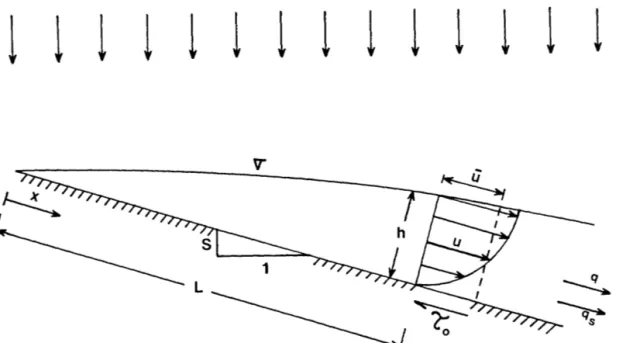
or turbulent and the surface can be either rough or smooth. The hydraulic characteristics of flow in a wide channel are shown in Figure 1. The main geometric variables are the plot length L and the slope S. The hydraulic variables are the rainfall intensity i, the flow depth h, the mean velocity u, the unit water discharge q, and the thickness of the laminar sublayer 6'. The parameter generally associ-ated with the sediment discharge q

8 is the bed shear stress t0 • While

the other properties are the gravitational acceleration g, the kine-matic viscosity v and the specific mass of water p and of sediments p .

s

2.2 Fundamental Equations

The two nonlinear partial differential equations derived by de Saint-Venant are basically used to solve the problem of gradually varied unsteady flows. The continuity equation is

oh - oh au

at + u ax + h ax

=

qo (1)

and the momentum equation including a lateral inflow component q

0 is: in which: au - au oh ot + u ax

=

g(S - Sf) - g ax = inflow rate

=

friction slope qo

h

(u -

v)

v

=

the velocity component along x of the lateral inflow.

(2)

Considering the principal terms of the momentum equation, the kinematic wave approximation has been most widely recommended (Wooding, 1965; Woolhiser, 1975). This approximation states that the friction slope is equal to the soil surface slope, or

(14)

5

il

l l l l l l l l

l

l l l

l

(15)

For the case of steady uniform flow conditions over an impervious surface, the continuity equation can be written:

q

=

uh

=

iL

The Reynolds number is defined as follows:

uh Re

=

_v

(4)

(5)

The energy loss equation given by Darcy-Weisbach is written as a function of the Darcy-Weisbach friction factor f:

The value of the friction factor f is a function of the Reynolds number and the relative roughness.

Three other important variables regarding resistance to flow and soil erosion are the bed shear stress r

0, the shear velocity U* and

the thickness of the laminar sublayer o' in turbulent flows. These variables are defined as:

! = pghS

0 (7)

u,.,

=

If

(8)

o'

= 11.6 v

U .... l~ (9)

This last variable has a physical significance since the ratio of o'/d delineates the type of turbulent flow as whether the boundary is

s

smooth or rough (see Figure 2). With varying Reynolds number and rela-tive roughness, the friction coefficient f will follow different laws. Four types of flow ranging from laminar flow to turbulent flow will be

(16)

(17)

examined: 1) laminar sheet flow; 2) turbulent flow over a smooth surface as given by the Blasius equation; 3) turbulent flow over a rough surface given by the Manning equation; and 4) turbulent flow over a rough surface with very small relative roughness as given by the Chezy equation. This last flow type is not very likely to occur in overland flow. It has been considered as a limiting case for which the Darcy-Weisbach friction factor (or Chezy C) remains constant. For each of these flow conditions, the principal variables related to soil erosion

(u,

h and t ) are defined as a function of slope and water discharge for

0

steady flow conditions.

2.3 Laminar Flow

Laminar flows with raindrop impact can be described by the Darcy-Weisbach equation (Eq. 6) in which the friction factor f is related to:

(1) the Reynolds number Re, (2) the surface friction coefficient k

0

without raindrop impact, and (3) two empirical coefficients A and b for raindrop impact. The following relationship is generally used:

K

f

=

_Re =

k + Aib

0

Re

As shown in Table I, the values of

(10)

k have been tabulated by

0

Woolhiser for various surface types and the value k

=

24

0 is

represen-tative of the smooth surface condition. Several sets of coefficients A and b have been obtained from experimental investigations and these values are indicated in Table II. The experimental data reported by Shen and Li are shown in Figure 3. These indicate that for a bare smooth surface, the flow is laminar for Re < 900 and the Blasius law is valid for turbulent flows over a smooth surf ace when Re > 2000. Chen's data in Figure 4 shows that laminar flows are observed for

5

(18)

9

Table I. Resistance parameters for overland flow (after Woolhiser, 1975).

Turbulent Flow

Laminar Flow Chezy

c

Surface k Manning n 1

0 (ft~/sec)

Concrete or Asphalt 24 108 .01 .013 73 - 38

Bare Sand 30 120 .01 .016 65 - 33

Graveled Surf ace 90 400 .012 - .03 38 - 18

Bare Clay-Loam Soil 100 500 .012 - .033 36 - 16

(eroded)

Sparse Vegetation 1000 4000 .053 - .13 11 5

Short Grass Prairie 3000 - 10,000 .10 .20 6.5 - 3.6

Bluegrass Sod 7000 - 40,000 .17 .48 4.2 - 1.8

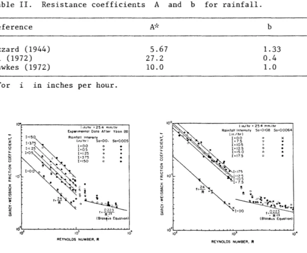
Table II. Resistance coefficients A and b for rainfall.

Reference

Izzard (1944) Li (1972) Fawkes (1972)

*For i in inches per hour.

-·

101cf...___.____..__._...._._..._10₁_ _...____. ... !04 REYNOLDS NUMBER, R A~·~ " 5.67 27.2 10.0

-

, ... : a u ;;::: u. w 8 z 0 ;:: u 10·' ~ :i:

~

w 3:. ~ cs 1cl 102 b 1.33 0.4 1.0 I in/hr • 25 4 mm/hr

Roinfol! Intensity So,0108 So=00064

(in./ hr) I=O.O + x I= 7.5 " ., I= 105 I• 12.5 I=15 0 I• 17.5 REYNOLDS NUMBER, R

Figure 3. Influence of rainfall intensity on the friction coefficient (after Shen and Li, 1973).

(19)

c ~ u " 0 i:: 104

.

"'

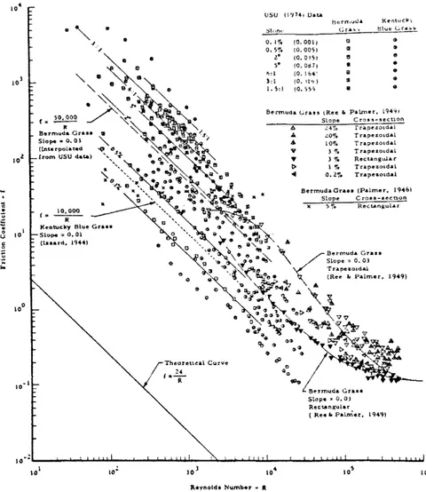
.J ~ • 101 r~ 102 10,000 C = -R 101 10° usu (1'1741 Uat.& tterniu<la. Kentuck',

Sl11nt· Gr&'.'11<» ~.lue Gr•::io!» 0. l'!e (0. 001) G Q O. S'!. (0. 005) ll

..

z• (0. 0 IS) !! e 5• (0. 0~7) • • li:I (0. 1&4: II ):l 10. ,l,,)

..

I. 5:! (O. ss; _"

Bermuda <.;rus (Ree I< Palm•<, l9491 Slope C ro,. !I-section

A 2:.4~0 !r~pez.01d•l

& lO'!o Trap•zo1dal

4' lO'lo Tnpezmda.l V 3 'lo Trapezoidal • 3 'lo Recta.nguh.r t> l 'lo Trapezoida.l ... a.

z,.

Tu.pe&o1dal Bermuda.Cira . . (Palmer, 1940) Slope Croas-•e-cnon S '• Rectil.ngul~r 1949) <>JO eQ \ . \ \ \ 0: ~o~, "eC>~ "

e

"o~:~,,,~~~.t.~Y

.. •• • ..

:"~~~

~C>~~~~

QQ ~ .,,.., Bermuda Gra.1• Slope = 0. OJ Rectangular ( Ree a. Pauner, 1949! 1o·Z._ __ ...__...,...._..., ... __ _...__.._...,...,....,..._ __ ... ..._...._...._ ... ...._ __ ...._--1....;._._~..._.--_...__.._ ... ...._..., 101 Reynold• Number • R

Figure 4. Influence of vegetation on the friction coefficient (after Chen, 1976).

For very low Reynolds numbers, the flow is laminar and the Darcy-Weisbach equation for that type of flow is given from Eqs. 6 and 10

(~~)

(11)

where K is the friction parameter for sheet flows.

Along a vertical profile, the shear stress and velocity

(20)

and t

=

t y 0 h - ~ (h2 2) u - Kv - y 11 (12) (13)

in which, t is the shear stress and u is the velocity at the distance y from the free surface. The main flow velocity determined from the integration of Eq. 13 gives:

ii

=(~)

s

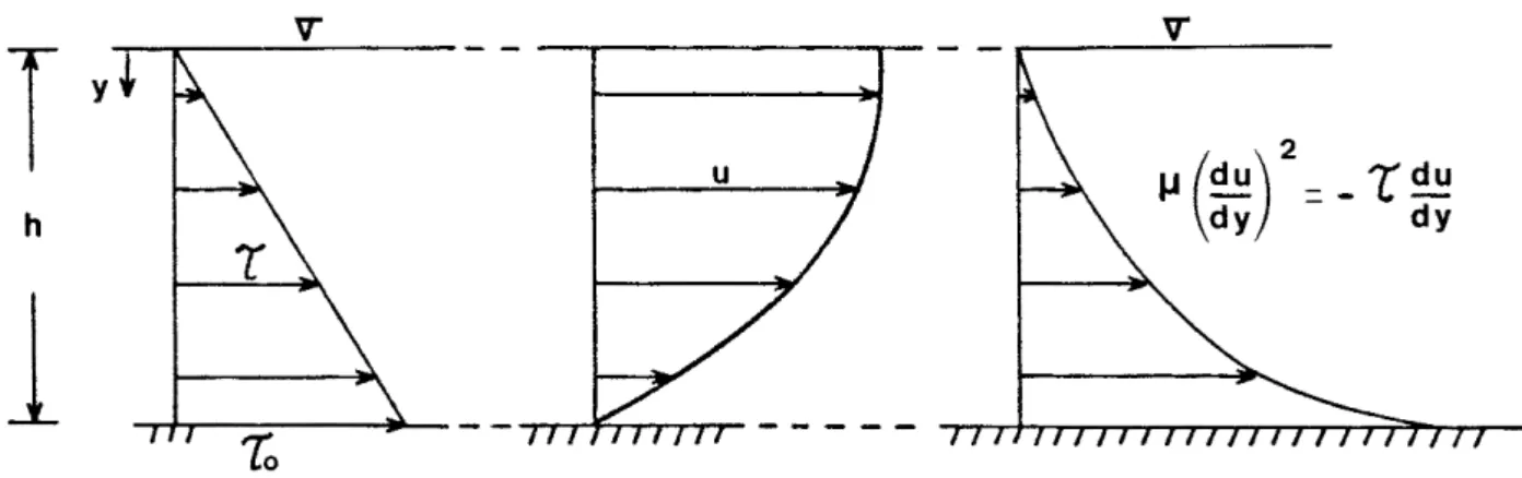
h2 (14)

The general equation for energy dissipation in three dimensions with no limitations on the boundary conditions has been reported by Lamb (1932). In the simplified case under consideration, the rate of energy dissipation $ reduces to:

$

=

µ

(:~)2

=

-t du _dy (15)

The profiles of shear stress (Eq. 12), velocity (Eq. 13), and rate of energy dissipation (Eq. 15) in laminar sheet flows are plotted in Figure 5.

The variables u, h and t for laminar sheet flows derived from

0

Eqs. 4, 7 and 11 are summarized in Table III for comparison with similar relationships valid under turbulent conditions.

2.4 Turbulent Smooth Flow

Turbulent flows (Re > 2000) for bare soil surfaces behave as hydraulically smooth when the thickness of the laminar sublayer given by

o'

=

11. 6 v /U..,., is much in excess of the size of soil particles d

s

(o'

> 3 d ). In this case, Keulegan (1938) derived an equation similar

s

(21)

T

h

1

v

µ

(du)

2

= -

r

du

dy dy

Figure 5. Shear stress, velocity, and energy dissipation profiles

(22)

13

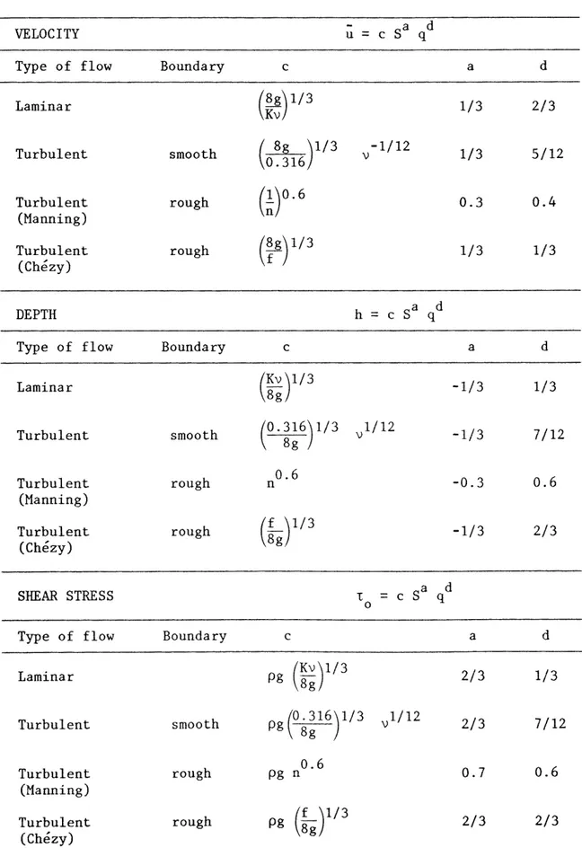
Table III. Summary of flow characteristics (velocity, depth, and shear stress).

VELOCITY u

=

c Sa q d

Type of flow Boundary c a d

Laminar

(~~)1/3

1/3 2/3

Turbulent smooth

(~)1/3

-1/12 1/3 5/12

0.316 \)

Turbulent rough

mo.6

0.3 0.4

(Manning)

Turbulent rough

(~g)

1/3 1/3 1/3

(Chezy)

DEPTH h

=

c S8 q d

Laminar

(~~)1/3

-1/3 1/3 Turbulent smooth

(0·~~6)1/3

\)1/12 -1/3 7/12 Turbulent rough n 0.6 -0.3 0.6 (Manning) Turbulent rough

(~g)l/3

-1/3 2/3 (Chezy) SHEAR STRESS 1: = c Sa q d 0

Laminar _{pg 8g}

(Kv

)113

2/3 1/3 Turbulent smooth pg

(o s!16) 113

\)1/12 _2/3 _7/12 Turbulent rough pg n 0.6 0.7 0.6 (Manning) Turbulent rough _{pg 8g}

(f

)1/3 2/3 2/3 (Chezy)

(23)

number is not too large, this equation can be approximated by the Blasius equation:

sf

=

o.316

(;h)~

-2 u 8gh

For turbulent smooth flows, the variables u,

(16)

h and t given in

0

Table III are derived from Eqs. 4, 7 and 16. The exponents of S for these variables are identical to those obtained for laminar sheet flows. 2.5 Turbulent Rough Flow

In turbulent rough channels (Re > 2000 for bare soil surface,

So' < d ) without bed forms, an increase of the Reynolds number (or

s

water discharge) raises the water level, and decreases the relative roughness and the friction factor. The logarithmic equation given by Keulegan (1938) is:

c

=

!¥

=

(17)

This equation is a theoretically sound resistance relationship for turbulent rough flows. Approximate power relationships such as the Manning equation, however, remain more useful to hydraulic engineers. Since both equations are in good agreement for open channel flows, the Manning equation (SI units) is used in this report:

u

=

!

h2/3

s

1/2

n f (18)

in which n is the Manning roughness coefficient. Strickler proposed the following formula to relate Manning n value to the median size, in feet, of the boundary roughness:

n

=

0.0342 d 116

(24)

15

The combination of Eqs. 4,

7,

and 18 gives the relationships for u, h, and t shown in Table III for turbulent rough conditions. One notices

0

that the relationship t a -2 u does not hold true for the Manning

0

relationship and the values of the exponents are slightly different than those derived from the Chezy relationship. The Manning n coefficient should be constant for uniform sediment roughness without bed forms.

When the relative roughness is small, the Darcy-Weisbach equation with constant friction factor is equivalent to the Chezy equation

(f

=

8g/C2 ) and after combining Eqs. 4, 6, and 7, the variables u, h, and t are written as a function of S and q. The resulting

expres-o

sions are listed in Table III. It is shown that t

0

-2

au while for the velocity u the exponents of q and S are identical and equal to 1/3.

2.6

Discussion

This analysis of the hydraulic characteristics is very instructive and the results summarized in Table III indicate clearly that when the velocity, the flow depth, and the bed shear stress are written in terms of discharge and slope, the exponent of the slope remains nearly the same for each variable under different flow conditions ranging from laminar to turbulent. The exponents of the slope for velocity, flow depth, and bed shear stress are respectively 1/3, -1/3, and 2/3. On the other hand, the exponent of the water discharge varies gradually under different conditions and for extreme conditions the exponent values differ by a factor 2. Moreover, the variation of the exponents of discharge for velocity and shear stress are in opposite directions for varying flow conditions. Indeed, for flow conditions changing from laminar to turbulent flows, the exponent of velocity varies from 2/3 to

(25)

1/3 while the exponent of shear stress varies from 1/3 to 2/3. This effect is extremely important if we consider the rate of sediment transport.

From this analysis it can be concluded that the transformation of bed-load equations from turbulent flow to laminar sheet flow will lead to completely different results whether the relationships are based on velocity or on bed shear stress.

III. SEDIMENT TRANSPORT EQUATIONS

This chapter deals with the sediment transport equations for rainfall erosion. Several approaches are investigated to obtain a theoretically sound relationship supported by experimental data. The method of dimensional analysis is first applied to the principal vari-ables related to soil erosion. Then, several empirical relationships are transformed into the general equation obtained by dimensional analy-sis. In the following section several sediment transport formulas are applied to turbulent smooth and laminar sheet flow conditions. Energy dissipation and stream power concepts are applied to sheet flows to derive theoretical sediment transport equations. The last section of this chapter summarizes the results obtained in this chapter. The range of the exponents of a sound relationship is defined and the results of various approaches are discussed.

3.1 Variables and Dimensional Analysis

Sheet erosion is the result of soil particles detachment and trans-port from raindrop impact and overland flow. Most of the eroded soil particles are transported downstream by runoff and the unit sediment discharge is a function of several variables. A relationship for

(26)

17

sediment transport by overland flow will be obtained from the analysis of the following variables:

(20)

in which t is the critical shear stress and d is the size of soil

c s

particles, and the other variables were defined previously. Among these variables, the first two (L, S) describe the geometry and the next five (i,

u,

h, q, T ) are flow characteristics including rainfall intensity.

0

The last six (tc, ds' p

8, p,

v,

g) are associated with soil and water

properties and the gravitational acceleration. The shear stress is difficult to measure in the field and is usually computed from other variables. In a river, the variables S, u, h and g are used to describe stream flows because the velocity and depth are generally more easily measured than the rainfall intensity and the length L. For this reason, Laursen (1956) suggested to reduce some sediment transport equations to a function of the variables u and h. On the other hand, in soil erosion problems, the variables i and L have a great physi-cal significance. The slope and unit water discharge can be more easily measured than the velocity and depth. Therefore, the variables S and q are more relevant than u and h to define a sediment transport relationship for overland flow. Elimination of the variables u and h is possible from the Darcy-Weisbach equation (Eq. 6) and the continuity equation q = uh.

The critical shear stress value t corresponds to the beginning

c

of motion of the sediment particles. Its evaluation remains a complex problem requiring further investigation, but the basic relationship gives the critical shear stress as a function of the particle size and the specific masses of water and sediment. The sediment size d can

(27)

be eliminated from a relationship between t

c and d s similar to

critical Shields number for laminar flow. In other words, the sediment size can be replaced by the critical shear stress in a sediment trans-port equation. In practice, the specific masses of water and sediment are nearly constant for particle sizes ranging from clays to gravels. In the case of aggregates, equivalent conditions of shear stress can be defined while keeping the same specific mass of sediment in the analy-sis. Therefore, to avoid redundancy of the variables, the constant value of and the relationship between t

c and d s enable us to

delete the variables p

s and d s from Eq. (20) , while keeping the

variable t .

c

Assuming ys constant, Eq. 20 thus reduces to

t c f ( q 8 , q, i , L , p , v ,

t ,

S) = 0 0 (21)

The following dimensionless groups are obtained from dimensional analysis after

L, p,

and v are selected as repeated variables

f (qs g, iL pv ' v ' v t c t 0

s)

=

o

(22)

The expected general solution gives the sediment transport term as a function of the product of the other variables in the form

tc)e . for

t '

0

(23)

In this equation, a,

B,

y,

o,

and e are experimental coeffi-cients and the sediment equations based on tractive force and stream power concepts are best represented by the term 1 - (t /t ).

(28)

19

Under dimensional form, this equation is transformed to

qs a

sf3

q

y

1.

.o

(1 - ::

t

(24) in which, - 6 a p L (1 ₌

vy+o-1

(25)

Equation 24 was obtained by Julien (1982) to describe the general relationship between sediment discharge and the principal flow vari-ables. The first three factors (S, q, i) represent the potential erosion or transport capacity by overland flow, which is reduced by the last factor essentially representative of the soil resistance to erosion. It is also seen that when !

c remains small compared to ! 0 '

the equation for sediment transport capacity is

(26)

For stream flows, the sediment transport equation is not a function of the rainfall intensity, and therefore,

o

=

0 in this case.

3.2 Empirical Equations

Quantitative evaluation of the coefficients a, ~'

y,

6 and e

can be obtained from several types of equations based on different vari-ables. The equations analyzed are those proposed by Musgrave (1947); Li, Shen and Simons (1973); and several regression equations obtained by Kilinc (1972) and others, including tractive force, stream power,

veloc-ity, and discharge equations. When these equations are a function of variables different than those of Eq. 24, the relationships in Table III for laminar flow are used for the variables u, h, and t , and the

0

Reynolds number is replaced by Re

=

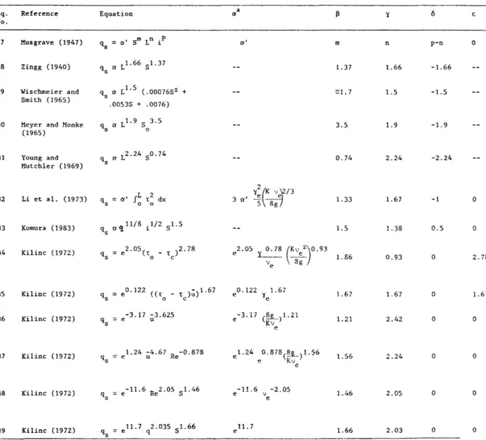
uh/v _{The results are shown in} Table IV, and it is found that none of the actual equations is complete

(29)

Table

IV.

Transformation of several erosion equations.

Eq. Reference Equation er a ~ y 6 i:;

No. 27 Musgrave (1947) _qs

=

a' Sm Ln ip a' m n p-n 0 28 Zingg (1940) _qser L 1. 66 S 1. 37 _1.37 _1.66 _-1.66 29 Wischmeier and q a Ll.S (.0007652 + ~n. 7 1.5 -1.5 Smith (1965) s .00538 + .0076)

30 Meyer and Monke _qsa Ll.9 S 3.5 3.5 1. 9 -1. 9

(1965) 0 31 Young and _qsa L2.24 80.74 o. 74 2.24 -2.24 Mutchler (1969) 2 q

=

a' IL t2 dx y (~/3 32 Li et al. (1973) 3 ' e e 1. 33 1.67 -1 0 s 0 0 a 5 8g 33 Komura (1983) _qser q 11/8 i 1/2 8i.5 LS 1.38 0.5 0 34 Kilinc (1972) q _s

=

e2.05(t _ t )2.78 e 2.05 1-_______ 0.78 (Kv ____!:.__ 2)0.93 _1.86 _0.93 ₀ _2.78 0 c ve 8g 35 Kilinc (1972)

=

eo.122 ((t - t );;)1.67 122 1.67 _1.67 _1.67 ₀ _1.67 qs 0 c ye 36 Kilinc (1972) _qs

=

e -3.17 -3.625 u e -3.17 (~)1.21 _Kv 1.21 2.42 0 0 e

37 Kilinc (1972) _qs

=

el.24 ~4.67 Re-0.878 e 1.24 o. 878(~-L)1. 56 l.56 2.24 0 0 e Kv

e

38 Kilinc (1972) _qs

=

e-11.6 Re2.05 81.46 e -11.6 v -2.05 1.46 2.05 0 0 e

39 Kilinc (1972) ₌e 11. 7 2.035 q 81.66 e 11. 7 1.66 2.03 0 0 3

(30)

21

since some coefficients are still zero. Consequently, for each particular equation, the number of variables is reduced owing to these zero values. From this analysis the main parameters are the slope S and the discharge q. The numerical values of the coefficient ~ vary from 1.2 to 1.9, and y varies from 1.4 to 2.4. These range of values will be referred to as the range of the empirical coefficients ~ and y for erosion equation by overland flow.

The well-known Universal Soil Loss Equation cannot be transformed directly into the general equation since the slope factor is written in a quadratic form. The equivalent exponent, however, is expected to vary between 1 and 2. Julien (1982) suggested an equivalent exponent value near 1.7. The Kilinc and Richardson equations cannot define the param-eters

6

and e since the overland flow rate is almost the same as the rainfall rate and also the bed tractive force is generally much in excess of the critical shear stress value. This analysis also shows that the number of independent parameters after transformation is the same as before transformation. For example, equations based on slope and length (Eqs. 28, 30 and 31) have two independent parameters, both before and after transformation, which imposes the condition 6 = -y. Considering equations having one independent parameter, for Eq. 34, e

=

3y and ~

=

2y; for Eq. 35, ~

=

y

=

e; and for Eq. 36, ~ = y. Further fundamental research is therefore needed to obtain a more complete description of the soil erosion rate. The coefficients of the general equation obtained by dimensional analysis are kept variable for the purpose of this study. Accordingly, the prediction from each equation will be possible, provided the proper set of coefficients is selected from Table IV. Fair estimates can be obtained from a

(31)

regression equation such as given by Kilinc (1972). Excellent results were obtained by Julien (1982) with the use of the discharge and slope formula (Eq. 39).

Soil erosion by overland flow does not remain absolutely uniform as assumed theoretically. The formation of rills locally increases the unit water discharge q such that on the whole area, the resulting erosion rate may be larger than for uniform flow conditions. The rill erosion data collected by Kilinc were analyzed by the writers and once the volume of rill erosion was subtracted from the total erosion, the following regression equation was obtained

Sl. 31 1. 93

qs a q (R2 = 0.96) (40)

This equation will be used for comparison with sediment transport equations for laminar sheet flow.

3.3 Sediment Transport Equations for Streams

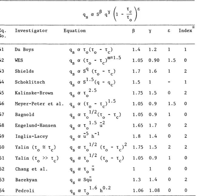
In this section, we propose to transform several of the well-known sediment transport equations originally derived for turbulent stream flows in order to determine whether they are applicable or not to laminar and turbulent conditions in overland flows. So many sediment transport equations in turbulent streams have been suggested by various investigators that it is almost impossible to consider all of them. This analysis includes the transformation of the equation suggested by Du Boys (1879), O'Brien-Rindlaub (1934), or WES (1935), Shields (1936), Schoklitsch (1934), Kalinske-Brown (1949), Meyer-Peter and Muller (1948), Bagnold (1956), Engelund-Hansen (1967), Inglis-Lacey (1968), Yalin (1977), Chang et al. (1967), Barekyan (1962), and Pedroli (1963). The Einstein bedload equation has not been treated separately

(32)

23

since it agrees very well with the Yalin and the Meyer-Peter and Muller equations.

A constant sediment grain size is assumed and the analysis is focused on the sediment transport capacity. Other constants such as the fluid properties or the gravitational acceleration are also deleted from the investigation. Particular attention is pointed at the values of ~

and y which are the exponents of the slope and water discharge in Eq. 24. For each of the types of flow described in Chapter 2, the results have been summarized in four corresponding tables: (a) laminar sheet flow (Table V); (b) turbulent flow over smooth surface as given by Blasius equation (Table VI); (c) turbulent rough flow described by Manning equation (Table VII); and (d) constant Darcy-Weisbach or Chezy

coefficient (Table VIII).

The last column of these four tables represents an index of fitness of these basic equations with the observed value of exponents. This index is equal to the number of parameters (~, y) enclosed within the ranges of empirical coefficients as determined in the previous section (1.2

<

~

<

1.9 and 1.4 < y < 2.4). The higher the index is, the best this equation should compare with observed data. Conversely, when the index is equal to zero, the given equation is expected to be a poor predictor for overland flow.

The sediment transport equations transformed give reasonable values of the parameter

B·

The value of

y,

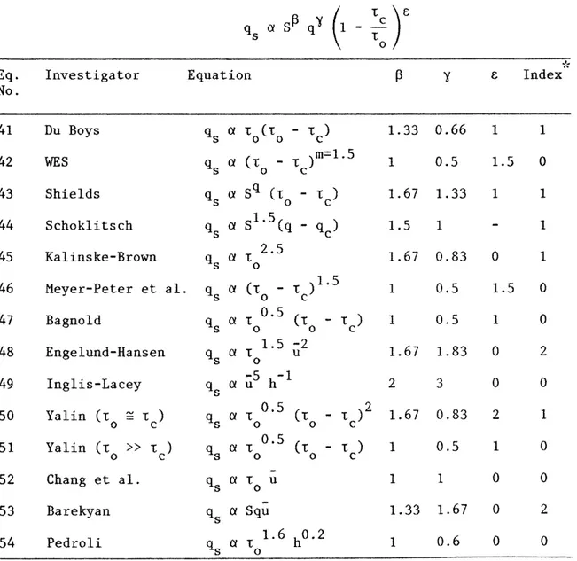
however, are generally is usually too small to fall within the range of empirical coefficients. The parameter £ is highly variable for these equations and further inves-tigation of incipient conditions are required to better define the critical shear stress and the parameter ~.

(33)

Table V. Transformed equations for laminar sheet flow. Eq.

No.

41 42 43

44

45 46 47

48

49

so

51 52 53 54 Investigator Du Boys

WES

Shields Schoklitsch Kalinske-Brown Meyer-Peter et al. Bagnold Engelund-Hansen Inglis-Lacey Yalin (t

=

t ) 0 c Yalin (t

»

t ) 0 c Chang et al. Barekyan Pedroli Equation q a t (t - t ) s 0 0 c ( t )m=l .5 qs a to - c qs a sq (t - t ) 0 c a

sl.

5(q - ) qs qc a t 2.5 qs o q a (t - t )1·5 s 0 c q a t 0•5 (t - t ) s 0 0 c -2 u t 0.5 (t - t )2 qs a o o c a t 0·5 (t - t ) qs o o c q 5 a t0 u qs

a

Squ a t 1.6 h0.2 qs o 1.33 0.66 1 0.5 1. 67 1. 33 1.5 1 1.67 0.83 1 0.5 1 0.5 1.67 1.83 2 3 1.67 0.83 1 0.5 1 1 1.33 1.67 1 0.6 1 1.5 1 0 1.5 1 0 0 2 1 0 0 0

*The index represents the number of exponents within the ranges: 1.2 < ~ < 1.9; and 1.4 < y <

2.4.

~·· Index" 1 0 1 1 1 0 0 2 0 1 0 0 2 0

(34)

25

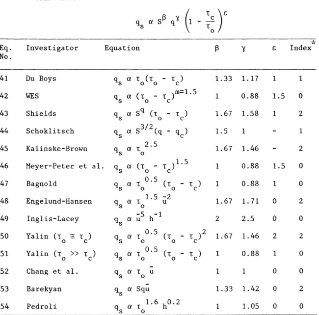
Table VI. Transformed equations for turbulent flow over a smooth boundary. Eq.

No.

41 42 43 44 45 46 47 48 49

so

51 52 53 54 Investigator Du Boys

WES

Shields Schoklitsch Kalinske-Brown Meyer-Peter et al. Bagnold Engelund-Hansen Inglis-Lacey Yalin (t

=

t ) 0 c Yalin (t

»

t ) 0 c Chang et al. Barekyan Pedroli Equation q Ci t (t - t ) s 0 0 c ( ,.. )m=l .S qs a to - Le q a sq

Ct -

i: ) s 0 c a s3/2Cq - ) qs qc q Ci t 2.5 s 0 q Ci (t - t )1·5 s 0 c q Ci t 0•5 (t - t ) s 0 0 c 1.5 -2 q 8 a t0 u qs a

ii

5 h - l Ci t 0·5 (t - t )2 qs o o c Ci t 0·5 (t - t ) qs o o c y

e

1. 33 1. 17 1 1 0.88 1.5 1.67 1.58 1 1.5 1 1. 67 1.46 1 0.88 1.5 1 0.88 1 1.67 1.71 0 2 2.5 0 1. 67 1. 46 2 1 0.88 1 1 1 0 1.33 1.42 0 1 1.05 0

*The index represents the number of exponents within the ranges:

1.2

<

~ < 1.9; and 1.4 <

y

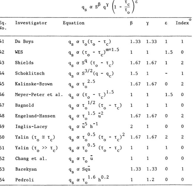
< 2.4. Index 1 0 2 1 2 0 0 2 0 2 0 0 2 0

(35)

Table VII. Transformed equations for turbulent flow over a rough boundary (Manning equation).

Eq.

No.

41 42 43 44 45 46 47 48 49 50 51 52 53 54 Investigator Du Boys

WES

Shields Schoklitsch Kalinske-Brown Meyer-Peter et al. Bagnold Engelund-Hansen Inglis-Lacey Yalin (t ~ t ) 0 c Yalin (t

»

t ) 0 c Chang et al. Barekyan Pedroli Equation q a t (t - t ) s 0 0 c ( )m=l .5 q a t - t s 0 c q

a

sq (t - t ) s 0 c SI. 5 ( ) qs a q - qc q a t 2.5 s 0 q a (t - t )1·5 s 0 c q a t 112

Ct -

t ) s 0 0 c 1.5 -2 q 8 a t0 u a

u

5 h-l qs t 1/2 (t - t )2 qs a o o c q a t l/ 2 (t - t ) s 0 0 c qs a t 0 u qs a Squ 1.6 h0.2 e 1.4 1.2 1 1.05 0.90 1.5 1. 7 1.6 1 1.5 1 1. 75 1.5 0 1.05 0.9 1.5 1.05 0.9 1 1.65 1. 7 0 1.8 1.4 0 1. 75 1.5 2 1.05 0.9 1 1 1 0 1.3 1.4 0 1.06 1.08 0

*The index represents the number of exponents within the ranges:

1.2 < ~ < 1.9; and 1.4 < y < 2.4. ~·-Index"' 1 0 2 1 2 0 0 2 2 2 0 0 2 0

(36)

27

Table VIII. Transformed equations for turbulent flow over a rough boundary (Chezy equation).

Eq.

No.

41 42 43 44 45 46 47 48 49 50 51

52

53 54 Investigator Du Boys WES Shields Schoklitsch Kalinske-Brown Meyer-Peter et al. Bagnold Engelund-Hansen Inglis-Lacey Yalin (t ::: t ) 0 c Yalin (t

»

t ) 0 c Chang et al. Barekyan Pedroli ( ttoc

)e

qs a

sf3

qY 1 -Equation q (l t (t - t ) s 0 0 c (t _ t )m=l.S qs

a

o c q 8 a sq (t -0 t ) c a s3/2(q - ) qs qc a t 2.5 qs o q a (t - t )1·5 s 0 c q

a

t 112 (t - t ) s 0 0 c 1.5 -2 qs a to u

a

u

5 h- 1 qs q 8

a

t0 u q 8 a Squ 1.6 h0.2 1.33 1 1.67 1.5 1.67 1 1 1.67 2 1.67 1 1 1.33 1 y 1.33 1 1 1.5 1.67 1 1 1.67 0 1 1.5 1 1 1.67 0 1 0 1.67 2 1 1 1 0 1.33 0 1.2 0

*The index represents the number of exponents within the ranges: 1.2 <

f3

<

1.9; and 1.4

<

y

<

2.4. Index 1 0 2 1 2 0 0 2 0 2 0 0 1 0

(37)

It can be concluded that most of these equations are not applicable to sediment transport by laminar sheet flow. Among the equations examined, the formulas proposed by Engelund-Hansen and Barekyan (Eqs. 48, 53) seem relevant for predicting soil erosion by overland flow. The formulas suggested by Shields, Kalinske-Brown and Yalin (Eq. 43, 45, 50) might also be considered but the parameter y is too small in the case of laminar sheet flow. The Inglis-Lacey equation (Eq. 49) seems fairly good for turbulent flow over rough boundaries, but clearly overestimates both parameters ~ and y under different flow conditions. The other equations generally underestimate the parameters

~ and y and are regarded as irrelevant for soil erosion.

3.4 Application of Energy, Work and Power Concepts to Sheet Flows

In the mid-eighteenth century the concepts of energy and work done were successfully applied to the motion of fluids with the significant contributions of Euler and Bernoulli. At that time, it was considered that no work was done by shear stress, no mechanical work was added to the fluid system and there was no heat transfer. One century later, Lord Kelvin (1845) discovered the concept of minimum kinetic energy for irrotational flow. The rate of dissipation of energy due to viscosity was then derived by Stokes (1851) and further developments were also reported by Lamb (1932) and Rouse (1959). As a result, when the shear stress components are included in the analysis, two sets of terms are added to the energy equation: (1) the total work done by shear stress; and (2) the dissipative work. The same analysis can also be extended to the work done per unit time called rate of work done, which correspond to the concept of power. At the beginning of the 20th century Gilbert (1914) formulated the major principles of work done by a stream, which

(38)

29

were later applied by Rubey (1933) to debris-laden streams under equilibrium conditions. In his paper, Rubey essentially derived and supported with experiments the following relationship:

= constant (55)

in which C is the sediment concentration; w is the fall velocity of particles, u is the mean velocity and Sf is the energy gradient. Another detailed analysis of sediment transport from the energy balance of solid and fluid particles emerged from Velikanov' s investigations between 1944 and 1956. His so-called gravitational theory, which has been summarized by Bogardi (1974) and Kondrat'ev (1959), is derived from the equilibrium of work done by gravity, settling of particles and friction of both fluid and solid phases. Bagnold (1960, 1966) studied the transport of sediment based on stream power per unit area t u

0

given by the product of the bed shear stress t and the mean velocity

0

u. His bed load equation is quite similar to Velikanov's (in Simons and Senturk, 1977) since they are both derived from similar principles. More recently Yang's papers (1967, 1972, 1973) emphasize on the rela-tionship existing between sediment transport and stream power per unit weight, given by the product of velocity and slope uS also called unit stream power. In his effort to obtain a dimensionless equation, he suggests the following relationship:

log C = I + J log (

~s

-

u~S)

(56)

in which u is the critical velocity; I and J are coefficients. c

(39)

u /u

is small and J

=

1. In the case of overland flow, Rooseboom and

c

Miilke (1982) show interesting results for turbulent flow with rough and smooth boundaries.

The scope of our investigation is to determine the values of the exponents

f3

and y, describing the sediment transport capacity in laminar sheet flows using energy and stream power concepts. The rela-tionships will be derived from three different ways: (1) rate of energy dissipation; (2) Bagnold stream power; and (3) unit stream power. The Bagnold stream power per unit area t u is obtained from Eqs.

4

and

7.

0

For laminar flow, the unit stream power uS is obtained from Table III. These expressions are:

t u = pgqS

0

us

=

(~)2/3

84/3 q2/3

(57)

(58)

Two different approaches referred to as global and local are used in this section. The former determines the sediment discharge from the mean characteristics of the flow. The latter describes the process at every point along the vertical profile and the sediment discharge equa-tion is thereafter obtained by integraequa-tion along the flow depth.

3.4.1 Rate of Energy Dissipation

A theoretical sediment transport equation for overland flow, is derived by assuming that the sediment concentration is proportional to the rate of energy dissipation. After substituting Eq. 13 into Eq. 15, one obtains

(40)

31

The local approach assumes that Eq. 59 is valid at every point along the vertical profile and the unit sediment discharge q

8 is

obtained by the following integral h

q =

f

Cu dy

s 0 (60)

After substituting the velocity equation for laminar flow Eq. 13

and the sediment concentration given by Eq. 59 into Eq. 60, the unit sediment discharge relationship is

a .e.&

(8g)

113

₈

4/3

5/3

qs

Kv

KV q (61)

Then assuming that in general,

p,

g,

K

and

v

are nearly constant gives

84/3 5/3

qs a q (62)

This is the main equation obtained from the rate of energy dissipa-tion. One may apply the global approach as well, which can be written in terms of the product of the mean velocity and the total energy dissipation rate:

- h q a u

I

<P <ly

s 0 (63)

After subs ti tu ting Eq. 59 and the velocity and depth for laminar flow (Table III), the integration of Eq. 63 leads to the same result as Eq. 62.

3.4.2 Stream Power Approach

Bagnold pointed out that the maximum transport efficiency is larger for laminar flow than for turbulent flow. If one assumes that his sediment transport relationship is valid for laminar overland flow, the global approach gives:

(41)

qs a to u - u w

(64)

For a given particle size, the fall velocity in clear water remains constant, and from the equations for velocity and shear stress for laminar flow (Table

III),

Eq.

64

transforms to

S4/3 5/3

qs Ci q (65)

This equation is the same as Eq. 62 derived from energy dissipation concept.

Another sediment transport equation based on stream power has been used in the past. This equation includes the critical shear stress t

c

and an exponent to the stream power term m - m

q a ((t - t ) u)

(66)

s 0 c

It is seen that when the critical shear stress t

c is small

compared to the bed shear stress t the corresponding equation for the

0

sediment transport capacity is written as follows

( - m 8m m

q a t u) a q

s 0 (67)

This means that the exponents of q and S are not independent but linked to each other because the original equation (Eq. 66) has only one degree of freedom. From the analysis of experimental data of rainfall erosion Kilinc (1972) obtained the value m

=

I.67 by regression analysis (Eq. 35).

3.4.3 Unit Stream Power

As mentioned previously, Yang's stream power equation can reduce to Rubey' s equation. Let us assume that the sediment concentration is

(42)

33

proportional to the product uS/w. Using the global approach, the sediment discharge is

q a Cq a us

s w q (68)

This relationship can only be derived by using the global approach since in this case the local approach erroneously means that the concentration is maximum near the surface. For a given size fraction (constant fall velocity), after substituting the velocity equation (Table III) in Eq. 68 gives

84/3 5/3

qs a q (69)

It is then concluded that for laminar sheet flows the three different approaches used to derive a sediment transport relationship (rate of energy dissipation, stream power and unit stream power) lead to the same power function of slope and discharge.

The following sediment transport equation based on unit stream power has also been suggested:

C a

((u - u

)S)N

c (70)

in which N is an exponent equivalent to J in Eq. 56 when w is con-stant. Here again, when the critical velocity

u, the sediment transport capacity is:

S4N/3 1+2N/3 q Ci q s u c is small compared to (71)

Since Eq. 70 has only one degree of freedom, the exponents of q and S are not independent though they might have different values. Unless there is a physical reason or theoretical evidence to support equations using one degree of freedom, a general regression

(43)

analysis aiming to determine the influence of the variables q and S separately should not be made with such restrictive equations. Other-wise, the exponents obtained from regression analysis represent a compromise value between two independent exponents. Fortunately, for soil erosion, Eqs. 66 and 70 can give fair approximation since the exponents of q and S do not differ considerably. Also, Eq. 39 in Table IV can approximately reduce to Eq. 71 when N ~ I. 3, which is within the range of previous observations by Yang (1972) on several streams (1.0

<

N

<

2.1).

3.4.4 Other Theoretical Equations

Another theoretical equation was suggested by Li, Shen and Simons (1973). This equation assumes that the pickup rate of particles is proportional to the square of the bed shear stress:

(32)

in which x is the longitudinal distance. As pointed out by Shen (1979), this equation can be reduced to Eq. 62, for laminar sheet flows. This soil erosion equation based on force equilibrium is therefore in agreement with those based on stream power and energy dissipation approaches.

3.5 Summary of Results and Discussion

The principal sediment transport capacity relationships for laminar flows are summarized in Table IX. The discussion of the results of this study is based on the comparison between several sediment transport capacity relationships for rainfall erosion given by q a

sf3

q Y. The

s

values of the exponents

f3

and y are compared for the different approaches used in this chapter. The equations are classified between

(44)

35

Table IX. Summary of sediment transport capacity equations in laminar sheet flow. Eq. Relationship q a s~ qy y No. s Theoretical 62 Energy dissipation 1.33 1.67 65 Stream power 1.33 1.67

69 Unit stream power 1.33 1.67

32 Li, Shen and Simons 1.33 1.67

EmEirical

28 Zingg (1940) 1.37 1.66

29 Universal soil-loss equation =i. 7 1.5

30 Meyer and Monke (1965) 3.5 1. 9

31 Young and Mutchler (1969) 0. 74 2.24

33 Komura (1983) 1.5 1.38

34 Kil inc (1972) _qs

=

_{f(t '} t ) 1.86 0.93

0 c

35 Kil inc (1972) _qs

=

_f_{(t '} t

ti)

1.67 1.67

0 c'

36 Kil inc (1972) _qs = f

Cli)

1.21 2.42

37

Kil inc (1972) _qs

=

tcli,

Re) 1.56 2.24

38 Kil inc (1972) _qs

=

f(Re, S) I.46 2.05

39 Ki line (1972) _qs

=

f(q, S) 1.66 2.03

40 Kilinc data (total erosion 1. 31 1. 93

minus rill erosion)

Transformed from Turbulent Flow E9,uations

41 Du Boys 1.33 0.66 42 WES 1.0 1.0 43 Shields I. 67 1.33 44 Schoklitsch 1.5 1.0 45 Kalinske-Brown 1.67 0.83 46 Meyer-Peter Muller 1.0 0.5 47 Bagnold 1.0 0.3 48 Engelund-Hansen I.67 1.83 49 Inglis-Lacey 2.0 3.0 50 Yalin (t

=-c )

1.67 0.83 51 Yalin (r0 >~ t ) 1.0 0.5 52 Chang et al. 0 c 1.0 1.0 53 Barekyan 1. 33 1.67 54 Pedroli 1.00 0.6

(45)

theoretical and empirical relationships for rainfall erosion, and also the transformation of turbulent flow relationships to laminar sheet flow conditions.

The theoretical equations give similar results

CB=

1.33 and

y

=

1. 67) and are recommended for laminar sheet flows without rills.

This relationship compares very well with Zingg relationship and with Kilinc data when the rill erosion is subtracted from the total erosion

(Eq. 40).

The exponents of the empirical relationships are shown in Figure 6

to vary within the following ranges 1.2 < ~ < 1.9 and 1.4 <

y

< 2.4.

The increase in these exponents is attributable to rill erosion which

varies for different soil types. As a first approximation, Eq. 39

CB

=

1. 66, y

=

2. 03) should be used when rill erosion is expected to

occur. This equation has been used by Julien (1982) to predict the

sediment transport capacity for both rainfall and snowmelt. This

equa-tion gave excellent results and is suggested unless a site specific

relationship is available. The use of the universal soil-loss equation

(Eq. 29) is also advocated though the exponent ~ is an approximation

of the quadratic function and the exponent

o

is negative (from

Table IV). Its wide use and calibration for various soil and climate

conditions enhance the applicability of this equation for predicting rainfall erosion.

Most of the turbulent sediment transport relationships transformed to fit the laminar sheet flow conditions give a wide range of exponents

B

and y, which values are usually outside the range of empirical

relationships. As mentioned in section 3. 3, i t can be concluded that

most of these equations are not applicable to rainfall erosion in

(46)

p

3.oT

THEORETICAL • ENERGY STREAM POWER - ll KILINC DATA

[J ZINGG 119401

Q WISCHMEIER & SMITH 119651 EMPIRICAL I !I YQUNG & MUTCHLER 119691

El KOMURA 119831

2.H I a KILINC 119721

~ RANGE OF EMPIRICAL VALUES

f) VALIN lt'0 ::::: 't"c I

<I VALIN (1:₀» tel

() CHANG & AL

•

BAREKYAN 2.01- 0 (t PEOROLI la

I

""

7 ""/

I

t> DU BOYS () WES TRANSFORMED

_e

_SHIELDS f)

e

K~;e~

Q SCHOKLITSCH f) KALINSKE- BROWN _w 1.5 l- Q

() MEYER PETER & MULLER --..J

l~

BAG NOLD

.,

v--><:

B

ENGELUND HANSEN (ii) _LACEY

1.0r

Q (t () l'!5 0.5 0.5 1.0 1.5 2.0 2.5 3.0 3.5 _?f

(47)

and Barekyan and to a certain extent, those of Shields, Kalinske-Brown and Yalin. In general, the exponent ~ of the stream sediment trans-port relationships is in agreement with the theoretical and empirical values. The exponents y for these bed-load equations, however, are outside the range of observed values.

IV. CONCLUSION

This report deals with sediment transport capacity relationships for overland flow. The objectives are mainly to determine: 1) whether equations derived for bed-load and total load in turbulent streams can be applied to laminar sheet flows and 2) whether stream power and energy dissipation concepts can be used to define soil erosion equations. The method used to achieve these goals was to point out the hydraulic characteristics of overland flow. Then the sediment transport variables were combined into a relationship for sediment transport

capacity of rainfall erosion

q

a

sB qy

s derived from dimensional

analysis. The exponents of this relationship were obtained from both theoretical analysis and transformation of bed-load equations. These exponents were then compared with empirical values obtained from experi-mental data. The principal conclusions of this investigation are summarized as follows.

Most of the sediment transport equations valid for turbulent flow in streams cannot be applied to rainfall erosion in laminar sheet flows. Among the equations examined, only those proposed by Engelund-Hansen and Barekyan (Eqs. 48 and 53) seem relevant for predicting soil erosion losses by overland runoff. The formulas suggested by Shields, Kalinske-Brown and Yalin (Eqs. 43, 45 and 50) might also be considered but the exponent of discharge is clearly too small in the case of laminar sheet

(48)

39

flow. The other equations generally underestimate the parameters ~

and y and are irrelevant to predict rainfall erosion.

The application of energy and stream power concepts to rainfall

erosion by laminar overland flow is conclusive. The theoretical

deri-vations for the case of uniform sheet flow are based on: (1) the rate

of energy dissipation; (2) the total stream power; and (3) the unit

stream power. These theoretical derivations lead to the same equation

for the sediment transport capacity ( q a Sl.33 q 1.67) .

s It is also

interesting to note that only the concept of energy dissipation can be

applied to every point along the vertical profile. The resulting

equa-tion is similar to an equaequa-tion derived from force equilibrium concepts

(Eq. 32), and show close agreement with regression equations based on

experimental data (Eq. 40). Equations based on energy dissipation and

stream power concepts are therefore recommended to predict the sediment

transport capacity of uniform sheet flows without rills. Some other

equations having one degree of freedom (Eqs. 32, 34, 35, 36, 67 and 70)

can give fair approximations of the rate of soil erosion from overland

flow. These equations are theoretically worthless since the exponents

of the main variables are interdependent.

The range of values of the exponents of slope ~ and of discharge

y were well-defined from this analysis. In the case of uniform laminar

sheet flows, the values ~

=

1. 33 and y

=

1. 6 7 are recommended to

define the sediment transport capacity of overland flow. In the cases

where rills develop, both exponents must be increased. The values

obtained from Eq. 39 (~

=

1.66 and

y

=

2.03) are suggested as a first

approximation unless a better empirical equation is available for the specific site and soil type under study.

(49)

Further theoretical analysis in this field should be focused on the processes of rill formation, considering the nonuniformity of flow depth and the difference between both laminar and turbulent flows.

(50)

41

BIBLIOGRAPHY

Alonso, C.V., W.H. Neibling and G.R. Foster. port capacity in watershed modeling.

Vol. 24, No. 5, 1981, pp. 1211-1220.

Estimating sediment trans-Transactions of the ASAE,

ASCE Task Committee. Sedimentation Engineering. Edited by V. Vanoni,

Manuals and Reports on Engineering Practice, No. 54. New York,

1977, pp. 190-214.

Bagnold, R.A. The flow of cohesionless grains in fluids.

of the Royal Society of London. Vol. 249, No.

pp. 235-297.