Traffic measurement and analysis

Traffic measurement and analysis

Henrik Abrahamsson September 1999

henrik@sics.se

Abstract

Measurement and analysis of real traffic is important to gain knowledge about the char-acteristics of the traffic. Without measurement, it is impossible to build realistic traffic models. It is recent that data traffic was found to have self-similar properties. In this thesis work traffic captured on the network at SICS and on the Supernet, is shown to have this fractal-like behaviour. The traffic is also examined with respect to which pro-tocols and packet sizes are present and in what proportions. In the SICS trace most packets are small, TCP is shown to be the predominant transport protocol and NNTP the most common application. In contrast to this, large UDP packets sent between not well-known ports dominates the Supernet traffic. Finally, characteristics of the client side of the WWW traffic are examined more closely. In order to extract useful informa-tion from the packet trace, web browsers use of TCP and HTTP is investigated includ-ing new features in HTTP/1.1 such as persistent connections and pipelininclud-ing. Empirical probability distributions are derived describing session lengths, time between user clicks and the amount of data transferred due to a single user click. These probability distributions make up a simple model of WWW-sessions.

Keywords: Traffic measurement, self-similarity.

SICS Technical Report T99:05

ISRN: SICS-T--99/05-SE ISSN: 1100-3154

Swedish Institute of Computer Science Box 1263, SE-164 29 Kista, Sweden

Traffic measurement and analysis

Henrik Abrahamsson

Examensarbete MN3 1999-09-15

Information Technology Department of Computer Systems

Uppsala University Box 325 SE-751 05 Uppsala

Sweden

This work has been carried out at SICS

Box 1263 SE-164 29 Kista

Sweden

Supervisor: Bengt Ahlgren Examiner: Jakob Carlström

Contents

1.0 Introduction 4

2.0 Self-similarity 6

2.1 Definitions ... 6

2.2 Methods for estimating the Hurst parameter ... 9

2.2.1 The R/S method ... 10

2.2.2 Variance-Time plot ... 11

2.2.3 The Periodogram method ... 11

2.2.4 Index of Dispersion for Counts ... 12

2.2.5 Implementation ... 12

2.3 Is SICS and Supernet traffic self-similar? ... 12

2.3.1 SICS ... 13

2.3.2 Supernet ... 16

2.4 Self-similarity - explanations and implications ... 18

2.4.1 Why self-similarity? ... 18

2.4.2 Implications ... 19

3.0 Results of traffic measurements 20 3.1 Introduction ... 20 3.2 SICS ... 23 3.2.1 Protocols ... 24 3.2.2 Packet sizes ... 27 3.3 Supernet ... 28 3.3.1 Protocols ... 29 3.3.2 Packet sizes ... 33 4.0 Modelling HTTP traffic 35 4.1 The HTTP protocols ... 35 4.1.1 HTTP/1.0 ... 36 4.1.2 HTTP/1.1 ... 37 4.1.3 An example ... 37 4.2 Methodology ... 40 4.2.1 Prior work ... 40

4.2.2 The packet trace ... 40

4.2.3 Sessions ... 41

4.2.4 User clicks ... 43

4.2.5 Tcpdump, Awk and Matlab ... 44

4.3.1 Model representation ... 45

4.3.2 Session lengths ... 45

4.3.3 Interarrival times of user clicks ... 46

4.3.4 Data transferred ... 47

4.3.5 Remarks ... 48

Abstract

Measurement and analysis of real traffic is important to gain knowledge about the char-acteristics of the traffic. Without measurement, it is impossible to build realistic traffic models. It is recent [18] that data traffic was found to have self-similar properties. In this thesis work traffic captured on the network at SICS and on the Supernet, is shown to have this fractal-like behaviour. The traffic is also examined with respect to which protocols and packet sizes are present and in what proportions. In the SICS trace most packets are small, TCP is shown to be the predominant transport protocol and NNTP the most common application. In contrast to this, large UDP packets sent between not well-known ports dominates the Supernet traffic. Finally, characteristics of the client side of the WWW traffic are examined more closely. In order to extract useful informa-tion from the packet trace, web browsers use of TCP and HTTP is investigated includ-ing new features in HTTP/1.1 such as persistent connections and pipelininclud-ing. Empirical probability distributions are derived describing session lengths, time between user clicks and the amount of data transferred due to a single user click. These probability distributions make up a simple model of WWW-sessions.

1.0 Introduction

Measurement and analysis of real traffic is important to gain knowledge about the char-acteristics of the traffic. Without measurement, it is impossible to build realistic theo-retical traffic models. The traditional telephone network could very successfully be analysed and modelled using applied mathematics such as stochastic processes. Espe-cially Poisson processes have been used which states that call arrivals are mutually independent and that the call interarrival times are all exponentially distributed, with one and the same parameter . Because of the success of voice network modelling and because Poisson processes have some attractive theoretical properties, the same approach have often been used when modelling data network traffic. Packet and con-nection arrivals have been assumed to be Poisson processes. But several studies [21] have shown that the distribution of packet interarrivals clearly differs from exponential and Leland et al. [18] showed that the burstiness on many timescales, observed in real traffic, can not be described with traditional Poisson-based traffic modelling. Instead they introduced statistically self-similar processes as a better way of modelling LAN traffic.

In this thesis work, network traffic on the Supernet and external traffic at SICS is ana-lysed. The traffic was captured using tcpdump [15]. Figure 1 shows the network at SICS. The machine running tcpdump (called network monitor in the figure) was listen-ing to the 100 Mbit/sec line connectlisten-ing all workstations at SICS with the gateway and in the end the SUNET network. This was used to capture all conversations between machines at SICS and the outside Internet world, for 24 hours. The packet trace was taken between 21:36 990414 and 21:40 990415 and includes more than 21 million packets.

The Supernet trace includes 15 million packets captured between 15:27 and 23:06 980423 on the Supernet in Sundsvall. Supernet consists of a mixture of Ethernet, ADSL (Asymmetric Digital Subscriber Line) and cable TV modems. Figure 2 shows the part of the network where the trace was taken. The trace includes all traffic between the ADSL-switch and the router and also the traffic between the two switches. ADSL provides approximately 7.6 Mbit/sec of downstream bandwidth (to the costumer) and 1.8 Mbit/sec of return bandwidth. For the cable modems each outgoing line from the switch makes up a segment where the active modems share 10 Mbit/sec of bandwidth.

The work is organized as follows. In Section 2 these packet traces are examined with respect to self-similarity. The section begins with definitions and a description of the methods used for estimating the degree of self-similarity. The result of applying these methods to the SICS and Supernet traffic data is presented in 2.3, and the section con-cludes with a discussion of what the possible causes and implications of self-similarity might be. In Section 3 the traffic is examined with respect to which protocols and packet sizes are present and in what proportions. To put the results in context this sec-tion begins with a brief outline of the TCP/IP protocol suite. The results show for instance the packet size distribution, the composition of the IP traffic during the time the traces were taken, which transport protocol is most common and what applications

Gateway Cisco 4500 Switch Corebuilder 3500 Network monitor Internet

Switch Switch Switch

stationWork stationWork

Figure 1. The network at SICS.

Internet Router Switch Network monitor Homes connected via ADSL Homes connected

via cable TV modem Switch

10 Mbit/sec 100 Mbit/sec

100 Mbit/sec

features in HTTP/1.1 such as persistent connections and pipelining. Empirical proba-bility distributions are derived describing session lengths, time between user clicks and the amount of data transferred due to a single user click. These probability distributions make up a simple model of WWW-sessions.

2.0 Self-similarity

In Section 2.1 the mathematics used are presented, leading up to the definition of self-similarity. Section 2.2 deals with the methods used for estimating the Hurst parameter that describes the degree of self-similarity. In Section 2.3 the result of applying these methods to the SICS and Supernet traces are presented, and in 2.4 these results are put in context when possible causes and implications of self-similarity are discussed.

2.1 Definitions

A random variable is a quantity that each time it is measured takes on one of a range of values. Particular values occur with different probabilities. Each separate measurement is referred to as an instance of the random variable. A generic random variable is denoted X, and xirepresents the ith instance of X. Unless otherwise stated, it is assumed

that there are a total of n instances. X is discrete if it assumes a finite or countable number of values. The random variable is continuous if it assumes all values in an interval according to a density function fX(x).

The Cumulative Distribution Function (CDF) of a random variable X tells the probabil-ity that an instance of X is less than or equal to a given value x.

,

The derivative of the CDF is called the probability density function (pdf) of X:

If X is discrete the CDF is not differentiable, and instead of the pdf the probability

func-tion px(k) = P(X=k), (k = 0,1,....) is used. This function tells the probability that an

instance of X is equal to a given value x. Some well-known distributions mentioned later on are:

Poisson distribution: (k=0,1,...),

Exponential distribution: and

Pareto distribution: , . F_X( )x = P X( ≤x) –∞ x ∞< < f_X( )x x d d F_X( )x = p_x( ) ek = –mmk⁄k! f_X( )x 1 m ----e–x m⁄ = x≥0 F_X( )x = P X( ≤x) = 1–(α x⁄ )β α β 0, ≥ x≥α

If in the Pareto distribution , then the distribution has infinite variance, and if then it has infinite mean. The Pareto distribution is an example of a heavy-tailed distribution. A distribution is said to be heavy-tailed if

, as .

In practical terms a random variable that follows a heavy-tailed distribution can give rise to extremely large values with non-negligible probability.

The cumulative distribution function or the density/probability function is used to get a complete description of a random variable. To get a description in more condensed form indices of central tendencies and dispersion is often used. The purpose of an index of central tendency is to summarize the data by a single number that (to be mean-ingful) should be representative of the major part of the data set. The most common used is the mean or expected value

,

where summation is used for discrete variables and integration for continuous random variables. An alternative is the median, which is obtained by sorting the observations in an increasing order and taking the observation that is in the middle of the series. To avoid drowning crossing a stream with an average depth of six inches, it is also impor-tant to know something about the indices of dispersion. These specifies the variability in a data set. Three popular alternatives are:

variance:

standard deviation:

coefficient of variation: .

Often it is also important to know if two random variables are dependent of each other. This can be examined using the simultaneous probability- or density function. But it is more often expressed as a single number using the covariance or the correlation

coeffi-cient. Given two random variables X and Y with means and , their covariance is

.

For independent variables, the covariance is zero. But the reverse is not true, it is possi-ble for two variapossi-bles to be dependent and still have zero covariance.The other measure of dependence between two random variables is the correlation coefficient:

β 2≤ β 1≤ P X( ≥x) cx∼ –β x→∞ β 0, ≥ E X( ) µ x_ip x( )_i i

∑

∫

When data is collected sequentially in time, a time series can be used for modelling and predictions. A time series [2] is a set of observations xt, each one being recorded at a

specified time t. In a discrete-time series the set of times in which observations are made is a discrete set, as is the case when observations are made at fixed time intervals.

Continuous-time series are obtained when observations are made continuously over

some time interval. The observations xtare often supposed to be instances of a random

variable X, and the time series is modelled as a stochastic process. A stochastic process

is a family of random variables with the same range. If T is an interval

of real numbers then the process is said to have continuous time, and if T is a sequence of integers it is said to have discrete time. The term time series is often used to mean both the data and the process of which it is a realization.

The autocovariance function of a process with finite variance is defined

by . A discrete time series is said to be

covari-ance stationary (or weak stationary or sometimes just stationary) if the expected value

of Xt is finite and equal to the same value m for all t, and it holds that

for all r, s, and t. That is, the series is covariance stationary if the mean is the same all the time and the dependence between all equally distanced pairs of observation is the same.

The autocovariance function can be redefined for a stationary process as a function of

just one variable: for all t and h. The

auto-correlation function of {X_t} is defined analogously as the function whose value at lag h

is for all t and h.

If a series is strict stationary then Xt has the same distribution for all t, which implies

that the expected value and variance are constant and the covariance is the same for all

h. A process is said to have stationary increments if the distribution of X(t+h)-X(t) only

depends on h.

For a detailed discussion of self-similarity and long-range dependence see Beran [4] and Willinger et al.[31], [33]. The description in this subsection follows those sources closely. There are a number of different, not equivalent, definitions of self-similarity.

The standard one states that a continuous-time process is

self-simi-lar with self-simiself-simi-lar parameter H if it satisfies the condition:

where the equality is in the sense of finite-dimensional distributions. While a process Y

satisfying this can never be stationary, that would require , Y is typically

assumed to have stationary increments. A second definition of self-similarity that is more appropriate in the context of standard time series, involves a stationary sequence

. Let , k = 1,2,..., X t( ) t T, ∈ { } X t( ) t T, ∈ { } γX(r s, ) = Cov X r( ( ) X s, ( )) r s, ∈T γX(r s, ) = γX(r+t s, +t) γX( )h = γX(h 0, ) = Cov X t( ( +h) X t, ( )) ρ_X( )h = γ_X( ) γh ⁄ _X( )0 = ρ X t h( ( + ) X t, ( )) Y = {Y t( ) t 0, ≥ } Y t( ) = ad –HY at( ) t 0 a 0 0 H 1≥ , > , < < Y t( ) = Y atd ( ) X = {X i( ) i 1, ≥ } X( )m ( )k (1 m⁄ ) X i( ) i=(k–1)m 1+ km

∑

be the corresponding aggregated sequence with level of aggregation m, obtained by dividing the original series X into blocks of size m and averaging over each block. The index k labels the block. If X is the incremented process of a self-similar process Y, that is X(i) = Y(i+1) - Y(i), then for all integers m,

.

If a stationary sequence satisfies this for all aggregation levels m,

then it is called exactly self-similar. It is said to be asymptotically self-similar if it holds

as . Similarly, a covariance-stationary sequence X(i), is called exactly

second-order self-similar if has the same variance and autocorrelation as X

for all m. It is said to be asymptotically second-order self-similar if it holds as .

A related notion is that of long-range dependence (LRD), which means correlations across large time scales. A stationary process is long-range dependent if its

autocorre-lation function is nonsummable:

Thus the definition of long-range dependence applies only to infinite time series. The two notions of long-range dependence and self-similarity are in general not equivalent. Long-range dependence is one of the ways in which self-similarity manifests itself [18] and self-similar processes are the simplest models with long-range dependence [21]. Self-similarity typically refers to scaling behaviour of the distributions of a continuous or discrete time process, while long-range dependence involves the tail behaviour of the autocorrelation function of a stationary time series. But since second-order self-similar also is defined in terms of autocorrelations, the terms long-range dependence and (exactly or asymptotically second-order) self-similarity are sometimes used in an interchangeable fashion, because both refers to the tail behaviour of the autocorrela-tions and are essentially equivalent [31].

One attractive feature with self-similar models is that the degree of self-similarity is expressed using only a single parameter, the so called Hurst parameter H. For

self-sim-ilar series with long-range dependence, 1/2 < H < 1, and as the degree of both

self-similarity and long-range dependence increases.

2.2 Methods for estimating the Hurst parameter

It is not possible to use the definition to check whether a finite traffic trace is self-simi-lar or not. Instead different features of self-simiself-simi-larity such as slowly decaying variances are investigated in order to estimate the Hurst parameter H. As mentioned in section 2.1, this parameter H can take any value between 1/2 and 1 and the higher the value the higher the degree of self-similarity. For smooth Poisson traffic the value is H=0.5. Here

X = md 1–HX( )m X = {X i( ) i 1, ≥ } m→∞ i≥1 m1–HX( )m m→∞ ρX( )h ρ_X( )h h=1 ∞

∑

and the Periodogram plot, and also the theory behind these methods, are described in detail by Beran [4] and Taqqu et al. [28]. Molnar et al. [20] describes the index of

dis-persion for counts method and also discuss how the estimation of the Hurst parameter

can depend on estimation technique, sample size, time scale and other factors.

Each packet captured with tcpdump has a timestamp. The traffic trace is divided up into time intervals (bins), for instance of size 100 ms. For each time interval the number of packets or bytes that arrived is counted. The resulting vector, with the number of pack-ets (or bytes) that arrived in each time interval, is input to all four of the methods described.

2.2.1 The R/S method

The R/S method is one of the oldest and most well known methods for estimating H. Let X_tdenote the number of packets that arrive at time t, i.e the number of packets in bin t, and let

be the cumulative inflow up to time j. The R/S-statistic or rescaled adjusted range is defined by the ratio

R/S = where

is called the adjusted range and

where

makes it possible to study properties that are independent of scale.

To determine the Hurst parameter H the ratio R/S is calculated for every possible, or a sufficient number of, values of t and k and log R/S is plotted against log k. The slope of a straight line fitted to the points in the plot, for instance by the least square method, is an estimation of the parameter H.

In practice the ratio R/S is not calculated for every possible t and k. Instead a number of equally spaced starting points t and a number of intervals (lags) k are chosen. Typically logarithmically spaced values of k is chosen because log R/S is to be plotted versus log

k. For each starting point t the ratio R/S is calculated for every lag k such that t+k <=

length of X. For small k one get many estimates of R/S but for large k one gets only a few, down to one, estimate of R/S.

Y_j X_i i=1 j

∑

∑

∑

The R/S method is known [28] to be biased towards H=0.7. It is biased upwards for small values of H and downwards for large values of H.

A number of questions arise: The ratio R/S can not in practice be calculated for every possible starting point t and lag k. What is a sufficient number of different values of t and k? The low and high ends of the plot is usually not used when estimating H because of the influence from short-range dependence in the low end and because there are too few points to make a reliable estimate in the high end. How to choose cut-offs? It turns out that slight changes in the values of the cut-offs and in the number of values of t and k don’t affect the estimate very much. The values used, when estimating H for the SICS and Supernet traces, are described in 2.2.5.

2.2.2 Variance-Time plot

Let X be a vector with the number of packets in each interval (bin). If for example the bin size has been chosen to 100 ms then X1 is the number of packets that arrived the

first 100 ms. Characteristic of long-range dependent processes is that the variance of the sample mean converges slower to zero than 1/n (the reciprocal of the sample size). It can be shown that

where c > 0.

This is what the variance-time plot method is based on and the actual method to esti-mate H is as follows:

First the mean of each pair of consecutive, non-overlapping bins are calculated and then the variance of these means is calculated. The 2-logarithm of the variance is plot-ted against the logarithm of the block size i.e 1. Then the same thing is done for blocks of size 4,8,16,..,length(X)/2 bins. The parameter H can be estimated by fitting a simple least squares line through the resulting points and using the relation slope = 2H - 2. The values for the smallest and largest block sizes are usually not included when esti-mating H. The problem is the same as for the R/S method. How to choose cut-offs?

2.2.3 The Periodogram method

The periodogram is defined as

whereυ is a frequency, N is the length of the series, and X is the time series. I(υ) is an estimator of the spectral density. A series with long-range dependence should have a periodogram which is proportional to |υ|1-2H_{close to the origin. An estimation of H is}

var X( ) cn_n ≈ 2H–2 I( )υ 1 2πN --- X j( )eijν j=1 N

∑

2.2.4 Index of Dispersion for Counts

The index of dispersion for counts is a common used measure for capturing the varia-bility of traffic over different time scales [18], [20]. For a given time interval t the index of dispersion for counts (IDC) is given by the variance of the number of arrivals during the interval divided by the expected value. The vector X with the number of packets that arrived in each interval (bin) is divided into non-overlapping blocks of length t.

IDC(t) is the variance of the number of packets in the blocks divided by the mean. IDC(t) is calculated for increasing block sizes t and for self-similar processes the

val-ues increases monotonically. The Hurst parameter H can be estimated by plotting log

IDC(t) against log t which results in an asymtotic straight line with slope 2H-1 [18].

To get a reliable estimate of IDC(t) the maximum block size is limited to 10% of the sample size [20]. Using non-overlapping blocks of length t at least about 10 values is needed to calculate the variance with acceptable confidence. Thus the calculated

IDC(t) value is getting more and more inaccurate as t increases. As a result, the IDC

plot becomes more and more noisy as t increases.

2.2.5 Implementation

The methods described for estimating the Hurst parameter were implemented using

Matlab. In Section 2.3, the results of applying these methods to the SICS and Supernet

traces are presented. But first the implementations were tested on traces, taken at the Bellcore Morristown Research and Engineering Center, which are available at the Internet Traffic Archive [14]. These traces are a subset of those analysed in Leland et

al. [18]. The estimates of the Hurst parameter that were obtained by applying the

meth-ods to the Bellcore data were compared to the results presented in [18] in order to con-firm that the implementations give reasonable results. For the R/S method different number of starting points t and lags k and different cut-offs were tried. Since the results were almost the same the method seems to be stable and when the results are presented in Section 2.3 the same values of these parameters are used. Twenty starting points were used and the lower cut-off was chosen as in Taqqu et al. [28] to 10^0.7. Besides this minimum, lags of sizes 10^0.75, 10^0.8,...,length(sample) were used. For the Vari-ance-Time method the problem is to decide which of the plotted points should be included when determining the slope. The points due to the smallest and largest block sizes were not used when estimating the Hurst parameter. For the IDC method the max-imum block size was restricted to 10% of the sample size when estimating H. The implementation of the Periodogram method seemed to work well for the traffic in the SICS trace when the proposed [27] lower 10% of the frequencies were used. But for the Supernet traffic and the Bellcore data the method sometimes gives absurd results. Therefore one Periodogram plot is shown for the SICS trace in 2.3.1, but all other results presented relies only on the R/S, Variance-Time and IDC methods.

2.3 Is SICS and Supernet traffic self-similar?

The methods described in 2.2 for estimating the Hurst parameter were used to investi-gate if the traffic captured in the SICS and Supernet traces are self-similar. The defini-tions of self-similarity and long-range dependence rely on the fact that the traffic, or the stochastic process describing the traffic, is stationary (or have stationary increments). This means for instance that the expected number of packets that arrive in 100 ms

should be the same irrespective of when the traffic is investigated. This would not be the case if 24 hour of traffic was examined at once, since the number of users and the load on the network varies during the day. The fact that it is not possible to tell with certainty whether or not the traffic is stationary and since it is difficult to distinguish stationary traffic with long-range dependence from certain non-stationary traffic with short-range dependence [13], at most one hour at a time of the traffic traces was exam-ined.

2.3.1 SICS

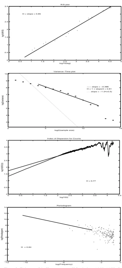
The hour between 14:00 and 15:00 of the trace was chosen for closer examination. This choice was somewhat arbitrary but it seems to be a “normal hour” of traffic (see also Figure 11 in Section 3.2). First the number of packets that arrived each 100 ms interval was counted and Figure 3 shows the resulting R/S plot, Variance-Time plot, IDC and Periodogram plots. With the R/S method the Hurst parameter was estimated to H = 0.85. The line fitted by least-square to the Variance-Time plot has slope -0.386 which gives an estimate of H=1+slope/2 = 0.81. The Index of Dispersion for Counts estimates

H to 0.77 and the Periodogram gives the value H=0.84. The methods don’t give exactly

the same result but the values are all clearly above 0.5, so the traffic is self-similar with

Hurst parameter .

Also, the byte traffic is self-similar with approximately the same H value. The number of bytes arriving in each time interval was counted and the R/S, Variance-Time and IDC methods were applied to this data. The results are shown in Table 1. This table also shows the resulting estimates of the Hurst parameter when different time intervals (bin sizes) were used, ranging from 10 ms to 1 second.

0 0.5 1 1.5 2 2.5 3 3.5 4 4.5 5 0 0.5 1 1.5 2 2.5 3 3.5 H = slope = 0.85 R/S plot log10(R/S) log10(lag) 0 5 10 15 3 4 5 6 7 8 9 10 Variance−Time plot log2(variance) log2(sample size) −−− slope = −0.386 H = 1 + slope/2 = 0.81 . . . slope = −1 (H=0.5) 0 0.5 1 1.5 2 2.5 3 3.5 4 4.5 0 0.5 1 1.5 2 2.5 3 3.5 4

Index of Dispersion for Counts

log10(t) log10(IDC(t)) H = 0.77 −12 −10 −8 −6 −4 −2 0 −4 −2 0 2 4 6 8 10 12 14 log(Periodogram) log(Frequency) Periodogram H = 0.84

Figure 3. Estimates of the Hurst parameter H for the hour 14:00 -15:00 of the SICS trace. At the top the R/S plot followed by Variance-Time plot, Index of Dispersion for Counts and at the bottom the Periodogram plot.

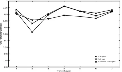
With the fact in mind that non-stationary traffic can be mistaken for self-similar station-ary traffic, even smaller parts of the trace was examined. The Hurst parameter was esti-mated for each of the six non-overlapping 10 minutes intervals between 14:00 and 15:00. The result is shown in Figure 4. None of the estimates is less than 0.75, so this hour of traffic is clearly self-similar.

So far only one hour out of the 24 hours of traffic captured in the SICS trace has been analysed. The Hurst parameter was estimated for each hour of the trace and the results are presented in Figure 5. The estimates are for packet traffic and the bin size 100 ms was used. All three methods show high values between hour 12 and 19. The trace started at 21:36 so that means between 8:30 and 16:30. Since this is also the time of the day when most people use the network it corresponds well with the findings of Leland

et al. [18] that the higher the load on the network the higher the degree of

self-similar-ity.

It is also notable that the three methods used sometimes give quite varying estimates of the Hurst parameter. Especially for the fifth hour between 01:36 and 02:36 when the R/S method estimates H to approximately 0.75, the Variance-Time plot gives a much lower value and the IDC method states that H=0.5, thus not self-similar at all.

Packets Bytes

Bin size: H_rs H_var H_idc H_rs H_var H_idc

0.01 s 0.85 0.85 0.77 0.83 0.86 0.78

0.1 s 0.85 0.81 0.77 0.85 0.82 0.78

1 s 0.86 0.76 0.77 0.87 0.78 0.78

Table 1. Hurst parameter estimates for the hour 14:00-15:00 of the SICS trace.

1 2 3 4 5 6 0.5 0.55 0.6 0.65 0.7 0.75 0.8 0.85 0.9 0.95 1 Time (10 minutes)

Hurst Parameter Estimates

IDC plot R/S plot Variance−Time plot

2.3.2 Supernet

The Supernet trace consists of 150 different files, each containing 100000 packets. A single file covers between two and three minutes of network traffic but there is always a short silence, were packets are missing, before the next file starts. These intervals of silence between files ranges from 150 to 580 ms. It is hard to know how much impact these silences have on the estimate of the Hurst parameter, but they don’t make the traf-fic less bursty. The hour between 19:42 and 20:42 was selected for a closer analysis since the silences between files were smallest during this hour.

The procedure is the same as for the SICS trace in section 2.3.1. The hour 19:42-20:42 was analysed in detail and the Hurst parameter was estimated using R/S plot, Variance-Time and IDC plots. The results are shown i Figure 6 and Table 2. The plots in the fig-ure show estimates of H for packet traffic using the bin size 100 ms. The R/S method gives the highest estimate H=0.90 while the Variance-Time and IDC methods estimates the Hurst parameter to 0.85 and 0.84. All methods estimates H to more than 0.75 for both packet and byte traffic and irrespective of bin size.

0 2 4 6 8 10 12 14 16 18 20 22 24 0.5 0.55 0.6 0.65 0.7 0.75 0.8 0.85 0.9 0.95 1 Time (hours)

Hurst Parameter Estimates

IDC plot R/S plot Variance−Time plot

Packets Bytes

Bin size: Hrs Hvar Hidc Hrs Hvar Hidc

0.01 s 0.82 0.88 0.84 0.78 0.83 0.79 0.1 s 0.90 0.85 0.84 0.87 0.86 0.79 1 s 0.89 0.79 0.84 0.88 0.76 0.79 0 0.5 1 1.5 2 2.5 3 3.5 4 4.5 5 0 0.5 1 1.5 2 2.5 3 3.5 4 H = slope = 0.9 R/S plot log10(R/S) log10(lag) 0 5 10 15 3 4 5 6 7 8 Variance−Time plot log2(variance) log2(sample size) −−− slope = −0.29 H = 1 + slope/2 = 0.85 . . . slope = −1 (H=0.5) 0 0.5 1 1.5 2 2.5 3 3.5 4 4.5 0 0.5 1 1.5 2 2.5 3 3.5 4

Index of Dispersion for Counts

log10(t)

log10(IDC(t))

H = 0.84

Figure 6. Estimates of the Hurst parameter H for the hour 19:42-20:42 of the Supernet trace. At the top the R/S plot followed by the Variance-Time and Index of Dispersion for Counts plots.

The six non-overlapping ten minutes intervals between 19:42 and 20:42 was investi-gated and the values of the Hurst parameter is shown in Figure 7. Finally, each hour in the trace from 15:27 to 22:27 was analysed. Only the packet traffic was examined using bin size 100 ms.The results are presented in Figure 8 and show that the lowest value of

H was approximately 0.75, but most estimates are above 0.85 and sometimes as high as

0.95. Thus, if the short silences between the trace files have little or no influence on the estimates then the traffic in the Supernet trace is clearly self-similar.

2.4 Self-similarity - explanations and implications

2.4.1 Why self-similarity?

The first findings of self-similarity in network traffic were met with scepticism, mainly because of the absence of physical explanations for the observed phenomena. It turned out that heavy-tailed distributions play an important part when explaining the causes of

1 2 3 4 5 6 0.5 0.55 0.6 0.65 0.7 0.75 0.8 0.85 0.9 0.95 1 Time (10 minutes)

Hurst Parameter Estimates

R/S plot Variance−Time plot IDC plot

Figure 7. Hurst parameter estimates for ten minutes intervals between 19:42 and 20:42 in the Supernet trace.

1 2 3 4 5 6 7 0.5 0.55 0.6 0.65 0.7 0.75 0.8 0.85 0.9 0.95 1 Time (hours)

Hurst Parameter Estimates

R/S plot Variance−Time plot IDC plot

self-similarity. These distributions have been found [32] for instance in sizes of files in a file system, inter-keystroke times when a person types, sizes of FTP bursts and in sizes and durations of bursts and idle periods in traffic between pairs of computers on an Ethernet LAN.

When trying to explain the empirically observed self-similarity, a structural modelling approach has been proposed by Leland et al. [18] and Willinger et al. [31], [33]. These structural models take into account specific features of the underlying network struc-ture and hence provide a physical explanation for the observed fractal nastruc-ture of aggre-gate network traffic. Aggreaggre-gate Ethernet LAN traffic can be separated into individual

source-destination pairs that represents the traffic flow between each active pair of

computers. These pairs are modelled as ON/OFF sources. The model assumes that a source alternates between an active and an idle state. During ON-periods packets are sent at a constant rate, and during OFF-periods no packets are transmitted. The length of the ON-periods are identically distributed, and so are the OFF-periods. The length of ON- and OFF-periods are independent. Willinger et al. [31], [33] presents a limit theo-rem that states that the superposition of many such ON/OFF sources captures the self-similar nature of aggregate LAN traffic, provided that the distribution of either the ON-or OFF-periods of an individual source-destination pair are heavy-tailed with infinite variance. In [33] a data set of self-similar Ethernet LAN traffic is analysed to validate the model, and it shows that a typical individual source-destination pair exhibits an apparent ON/OFF structure and that the distribution of the ON/OFF periods satisfy the heavy-tailed property. Thus self-similar LAN traffic can be constructed by multiplex-ing a large number of ON/OFF sources that have heavy-tailed ON or OFF period lengths.

Traffic carried over wide-area networks such as the Internet differs from LAN traffic in some fundamental ways that makes structural modelling more complicated. WANs are generally more heterogeneous and they have to cope with delays associated with obtaining and adapting to feedback on current network conditions, which introduce additional structure to the flow of packets. Structural modelling approaches for WAN traffic have been proposed by Willinger et al. [33], Paxson et al. [21] and Feldmann et

al. [11]. These models attempt to explain the self-similar nature of aggregate WAN

traffic at the packet level in terms of the characteristics of the main applications (e.g. HTTP, FTP and Telnet). The structural models are based on a construction called the

M/G/ model, where session arrivals are assumed to be Poisson, session durations are

heavy-tailed and packets are generated at a constant rate for the duration of a session. These models are shown to be partly valid for todays WAN traffic, but a more flexible traffic behaviour within sessions is needed. Multifractals, described by Feldmann et al. [11], [12], is another approach to describe and understand the dynamics of WAN traf-fic.

Thus, it seems like the self-similarity in network traffic can be explained simply in terms of the nature of the traffic generated by individual sources.

2.4.2 Implications ∞

change its behaviour but it changes the knowledge about real traffic and also the way in which traffic is modelled. It has lead many [21] to abandon the Poisson-based model-ling of network traffic for all but user session arrivals. Real traffic, well described as self-similar, has a “burst within burst” structure that cannot be described with the tradi-tional Poisson-based traffic modelling.

Erramilli [10] shows, using trace-driven simulation experiments, that long-range dependence in packet traffic has measurable and practical impact on queueing behav-iour. That long-range dependence is of crucial importance for buffer sizing, admission control and rate control, and if ignored typically results in too optimistic performance predictions and inadequate network resource allocation.

It should be emphasized that there is no total consensus among researchers about the importance of self-similarity and long-range dependence. The first fractal traffic mod-els were met with scepticism. Mainly because of the absence of physical explanations, but also because it was preceded by short-lived trends of using fractals in many other areas, such as economics, hydrology and biophysics. But not many articles have been published recently that argue against the use of self-similarity in network modelling. Grossglauser and Bolot [13] does not question the evidence that network traffic exhibit properties of self-similarity and long-range dependence, but debate about their practi-cal impact on network and application performance. They argue that processes with the same correlation structure (for instance LRD) can generate vastly different queueing behaviour. Therefore it is also important to consider other parameters for accurate per-formance predictions, such as the marginal distribution of the arrival process and the finite range of time scales of interest in performance evaluation.

3.0 Results of traffic measurements

Besides the question whether traffic is self-similar or not, it is also interesting to know what protocols and packet sizes are present and in what proportions. These questions are discussed in this section and the results of traffic measurements are presented. To put these results in a context, Section 3.1 gives a brief outline of the TCP/IP protocol suite. It also describes how information about protocols and packet sizes were obtained. In Section 3.2 the packet trace taken at SICS is analysed and 3.3 gives the results of the Supernet trace.

3.1 Introduction

This section gives a brief outline of the TCP/IP protocol suite. The description follows Stevens [25].

Networking protocols are normally developed in layers, each having a different respon-sibility. The TCP/IP protocol suite is a 4-layer system with different protocols at these layers. The link layer normally includes the device driver in the operating system and the corresponding network interface card in the computer. Together they handle all the hardware details of physically interfacing with the cable. The network layer handles the movement of packets around the network. The transport layer provides a flow of data between two hosts and the application layer handles the details of the particular appli-cation.

TCP (Transmission Control Protocol) and UDP (User Datagram Protocol) are the two predominant transport layer protocols. Both use IP (Internet Protocol) as the network layer. TCP provides a connection-oriented, reliable, byte stream service to the applica-tion layer. SMTP (Simple Mail Transfer Protocol) for transferring electronic mail mes-sages, Telnet for remote login and FTP (File Transfer Protocol) are some well-known applications that use TCP. UDP is a simpler, unreliable, transport protocol that sends and receives datagrams for applications. UDP is for instance used by DNS (Domain Name System).

IP, ICMP (Internet Control Message Protocol), and IGMP (Internet Group Manage-ment Protocol) provide the network layer in the TCP/IP protocol suite. IP is the main protocol at the network layer and it defines the IP datagram as the unit of information passed across an internet and provides the basis for connectionless, best-effort packet delivery service. It is used by both TCP and UDP. It is also possible for an application to access IP directly. ICMP is an integral part of IP that handles error and control mes-sages. Gateways and hosts use ICMP to send reports of problems about datagrams back to the original source that sent the datagram. ICMP also includes an echo request/reply used to test whether a destination is reachable and responding. Although ICMP is used primarily by IP, it is possible for an application to also access it. For instance the Ping program uses ICMP. IGMP is used by hosts and routers that support multicasting - the sending of a UDP datagram to a group of hosts. IGMP lets all the systems on a physical network know which hosts currently belong to which multicast groups. This informa-tion is required by multicast routers, so they know which multicast datagrams to for-ward on which interfaces. The positioning of the ICMP and IGMP boxes in Figure 9 is not obvious. It shows them at the same layer as IP, because they really are adjuncts to IP, but ICMP and IGMP messages are encapsulated in IP datagrams.

ARP RARP ICMP IP IGMP TCP UDP Hardware interface User process (PING) User process (Telnet, FTP) User process (DNS) User process media application transport network link

addresses used by the network interface. ARP provides a dynamic mapping from an IP address to the corresponding hardware address. RARP is the protocol a diskless machine uses at start-up to find its IP address. The machine broadcasts a request that contains its physical hardware address and a server responds by sending the machine its IP address. Also ARP and RARP are somewhat difficult to position in the layer hier-archy. In Figure 9 they are at the same layer as the Ethernet device driver, but they both have their own Ethernet frame type like IP datagrams.

When an application sends data, it is sent down the protocol stack, through each layer, until it is sent as a stream of bits across the network. Each layer adds information to the data by adding headers to the data that it receives. Figure 10 shows the Ethernet frame that results from an application using TCP. The result would have been similar if UDP were used but the UDP header is only 8 bytes compared to the 20 byte TCP header. When an Ethernet frame is received at the destination host it starts its way up the proto-col stack and all headers are removed by the appropriate protoproto-col.

A physical property of an Ethernet frame is that the size of its data must be between 46 and 1500 bytes. The network interface sends and receives frames on behalf of IP, ARP, and RARP. To identify which protocol generated the data a 16-bit frame type field in the Ethernet header is used. TCP, UDP, ICMP, and IGMP all send data to IP. IP stores an 8-bit value in the protocol field of its header, to indicate the layer to which the data belongs. A value of 1 is for ICMP, 2 is for IGMP, 6 indicate TCP, and 17 is for UDP. Similarly, many different applications can be using TCP and UDP at the same time. Both TCP and UDP use 16-bit port numbers to identify applications. The source and destination port numbers are stored in the header. Servers are normally known by their

well-known port number. For example, every Telnet server is on TCP port 23.

The unit of data that TCP sends to IP is called a TCP segment, the data that IP sends to the network interface is called packet or IP datagram, and the stream of bits that flows across the Ethernet is called a frame. But here the word packet will be used in a wide sense to cover all of these.

To get information about packet sizes the tcpdump software were used with the -e option to print the link-level header on each dump line. Suitable tcpdump expressions were chosen to select which packets should be read from the dumpfile in order to get information about protocols. For example the command:

tcpdump -e -r dumpfile port telnet

selects all Telnet packets in the file dumpfile and for each of them prints header infor-mation like Ethernet header IP header TCP

header application data

Ethernet trailer

14 bytes 20 bytes 20 bytes 4 bytes

Ethernet frame 46 to 1500 bytes

21:38:09.805840 [link-level info in hex] ip 60: src_host.sics.se.17209 > dst_host.se.telnet: . ack 1 win 32696 (DF)

showing the timestamp, link-level header information in hex, the packet size including the Ethernet header, source and destination IP addresses and ports etc. The UNIX com-mands awk and egrep were used to get timestamps and packet sizes from each dump-line.

3.2 SICS

The 24-hour packet trace taken at SICS contains header information from more than 21 million packets with a total of almost 7.6 Gigabyte (data included). Only external traf-fic, conversations between machines at SICS and the outside world, was captured using

tcpdump.The utilization of the network varied a lot during the time the trace was taken.

Figure 11 shows the number of packets that arrived each minute. Figure 12 shows the byte traffic.

There was a maximum of 64971 packets in one minute at 10:31 and a minimum of 3543 packets at 00:52. These 3543 packets together contained 364234 bytes which also is the minimum number of bytes that arrived in one minute. The maximum was 39468753 bytes at 17:04. 0 200 400 600 800 1000 1200 1400 0 1 2 3 4 5 6 7 x 104 _{Packets/minute} Packets (00:56) (04:16) (07:36) (10:56) (14:16) (17:36) (20:59) (21:36)

Figure 11. External packet traffic at SICS.

0.5 1 1.5 2 2.5 3 3.5 4 x 107 Bytes/minute Bytes

To be able to express the load in the more common units the number of packets and bits per one-second bin was counted. The maximum was 33.36 Mbit/sec and 4170 packets/ sec. The minimum was 13.13 Kbit/sec or 9 packets/sec and the mean was 0.705 Mbit/ sec and 245 packets/sec.

3.2.1 Protocols

The two tables below show the proportions in which the lower layer protocols appeared in the packet trace taken at SICS. The first shows IP versus non-IP traffic and the sec-ond shows these results in more detail.

ICMP, IGMP and the transport protocols TCP and UDP all use IP, so the first five rows in the table below is the IP traffic. The amount of ARP, RARP and other traffic not using IP is presented in the following three rows.

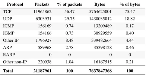
TCP is the transport layer protocol that dominates the traffic with 56% of the packets and 75% of the bytes. Almost 30% of the packets and 19% of the bytes in the trace taken at SICS is UDP. Together TCP and UDP stands for 86% of the packets and 94% of the bytes. Note that the Other IP category have more than 8% of the total number of packets. These are IP packets not due to any application using TCP or UDP at the transport layer and not ICMP or IGMP packets. A closer examination shows that most of the traffic in the Other IP category is due to IPv6 and IP in IP. As mentioned in Sec-tion 3.1 the IP header includes an 8-bit value in the protocol field which identify the next level protocol. 83% of the Other IP packets (comprising 57% of the bytes) have a protocol field value of 41, which is the IPv6 protocol. So, approximately 7% of the total number of packets (and 2.5% of the bytes) is IPv6 packets sent in ordinary IPv4 packets. 16% of the Other IP packets and 41% of the bytes is due to IP in IP. That is IP packets encapsulated (carried as payload) within other IP packets. Encapsulation is a means to alter the normal IP routing by delivering packets to an intermediate destina-tion that would otherwise not be selected based on the destinadestina-tion address in the

origi-Protocol Packets % of packets Bytes % of bytes

IP 20377055 96.17 7586281725 99.32

non-IP 810906 3.83 51565643 0.68

Total 21187961 100 7637847368 100

Table 3. IP and non-IP traffic in the SICS trace.

Protocol Packets % of packets Bytes % of bytes

TCP 11965862 56.47 5764625001 75.47 UDP 6303931 29.75 1438035012 18.82 ICMP 156169 0.74 13209489 0.17 IGMP 154166 0.73 30929559 0.40 Other IP 1796927 8.48 339482664 4.44 ARP 589968 2.78 35398128 0.46 RARP 0 0 0 0 Other non-IP 220938 1.04 16167515 0.21 Total 21187961 100 7637847368 100

nal IP header. When the encapsulated packet arrives at this intermediate destination it is decapsulated, yielding the original IP packet which is sent to the destination indi-cated by the original destination address. This use of encapsulation and decapsulation of a packet is called tunneling. A common application is multicasting.

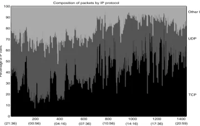
The composition of the IP traffic during the time the trace was taken can be seen in the figures below. Figure 13 shows composition of packets and Figure 14 composition of byte volume by IP protocols. The Other IP category here includes ICMP and IGMP.

The TCP traffic comprises a large part of the traffic but, compared to recent measure-ments on Internet backbone [6],[29] where TCP averages about 95% of the bytes and 90% of the packets, the external traffic at SICS also includes a lot of UDP and other traffic.

To get an idea of which application protocols are most used, the source and

destination-200 400 600 800 1000 1200 1400 0 10 20 30 40 50 60 70 80 90 100 Percentage of IP traffic (00:56) (04:16) (14:16) (17:36) (20:59) TCP UDP Other IP (07:36) (10:56) (21:36)

Composition of packets by IP protocol

Figure 13. Compostion of packets in the SICS trace by IP protocol.

200 400 600 800 1000 1200 1400 0 10 20 30 40 50 60 70 80 90 100 Percentage of IP traffic (00:56) (04:16) (14:16) (17:36) (20:59) TCP (07:36) (10:56) (21:36) Other IP UDP Composition of byte volume by IP protocol

then obtained using tcpdump with appropriate boolean expressions. Table 5 shows these results but also information about some well known protocols, like Telnet for instance, that don’t comprise a very large part of the traffic.

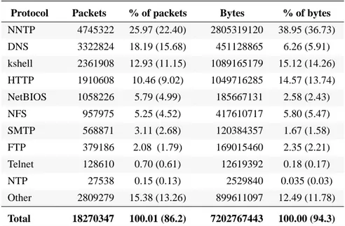
The third column shows the percentage of all TCP and UDP packets and the figures put in parenthesis is percentage of the total number of packets. The total number of TCP and UDP packets are 18269793 with a total of 7202660013 bytes. There are some traf-fic (554 packets actually) between the NetBIOS ports and the domain or nfs ports, so some packets are counted for twice. The Other category have more than 15% of the TCP and UDP packets spread among a lot of different ports, non of which represents more than 3% of the packets.

The most common application protocol is the NNTP (Network News Transfer Proto-col). More than 22% of all packets are due to NNTP, which is an application protocol that uses TCP to distribute news articles between cooperating hosts.

The second most common application is DNS (Domain Name System), the on-line dis-tributed database system used to map human-readable machine names into IP

addresses. More than 15% of the total number of packets in the trace is DNS and almost 6% of the bytes. DNS uses both TCP and UDP. A DNS client (called resolver) is normally part of a client application, for example, a Telnet client, an FTP client, or a WWW browser. The resolver sends a single UDP datagram to a DNS server requesting the IP address associated with a domain name. The reply is normally a single UDP dat-agram from the server, but if the reply exceeds 512 bytes only the first 512 bytes are returned along with a flag indicating that more information is available. The client then resends the query using TCP and the server returns the entire reply using TCP [26]. The TCP port 544, kshell (Kerberos remote shell), is the third most common port in the SICS trace. It is used for secure remote login and file transfer.

HTTP (Hypertext Transfer Protocol) is the basis for the World Wide Web (WWW). HTTP messages are transported by TCP connections between clients (web browsers)

Protocol Packets % of packets Bytes % of bytes NNTP 4745322 25.97 (22.40) 2805319120 38.95 (36.73) DNS 3322824 18.19 (15.68) 451128865 6.26 (5.91) kshell 2361908 12.93 (11.15) 1089165179 15.12 (14.26) HTTP 1910608 10.46 (9.02) 1049716285 14.57 (13.74) NetBIOS 1058226 5.79 (4.99) 185667131 2.58 (2.43) NFS 957975 5.25 (4.52) 417610717 5.80 (5.47) SMTP 568871 3.11 (2.68) 120384357 1.67 (1.58) FTP 379186 2.08 (1.79) 169015460 2.35 (2.21) Telnet 128610 0.70 (0.61) 12619392 0.18 (0.17) NTP 27538 0.15 (0.13) 2529840 0.035 (0.03) Other 2809279 15.38 (13.26) 899611097 12.49 (11.78) Total 18270347 100.01 (86.2) 7202767443 100.00 (94.3)

and servers. HTTP dominates the information exchange on the Internet. Measurements on Internet backbone [6], [29], shows that HTTP comprises 75% of the overall bytes and up to 70% of the overall packets. But in the trace taken at SICS less than 10% of all packets are HTTP.

NetBIOS (Network Basic Input Output System) in the table above refers to all packets with source or destinationports netbios-ns 137 (nameservice), netbios-dgm 138 (data-gram service) or netbios-ssn 139 (session service). Put together these packets make up about 5% of the traffic. NetBIOS was originally developed by IBM as an Application Program Interface (API) for IBM PC programs to access LAN facilities. In the TCP/IP internet, NetBIOS refers to a set of guidelines that describes how to map NetBIOS operations into equivalent TCP/IP operations.

Another 5% of the traffic is due to NFS (Network File System), a protocol that uses IP to allow a set of cooperating computers to access each other’s filesystems as if they were local. SMTP, FTP and Telnet all have low byte and packet percentage. Together they make up 5-6% of the packet traffic. FTP includes traffic using both the ftp and the ftp-data ports. NTP (Network Time Protocol) is a protocol used for maintaining the clocks for a group of systems on a LAN or WAN to within millisecond accuracy. NTP constitutes only 0.13% of the packets.

3.2.2 Packet sizes

The smallest packets in the trace were 60 bytes and the largest 1514 bytes. Figure 15 below shows the relative frequency of packet sizes including the 14 byte Ethernet header.

The ten most common packet sizes are 60, 566, 1514, 98, 86, 66, 87, 92, 122 and 225 bytes. There are peaks at sizes 60, 566 and 1514 bytes. The small packets, 60 bytes in length, include TCP acknowledgement packets, TCP control packets such as SYN, FIN and RST packets, and Telnet packets carrying single characters (keystrokes of a telnet session). A packet containing a TCP acknowledgement does not include any data except for the TCP and IP headers (20 +20 = 40 bytes) so the packet size of 60 bytes is

0 200 400 600 800 1000 1200 1400 1600 0 0.05 0.1 0.15 0.2 0.25 0.3

External traffic 990414 21:36:28 to 990415 21:40:01 at SICS Total number of pakets:21187961 Min size:60 Max size:1514

Packet sizes

packet size (bytes)

relative frequency

Many TCP implementations use 512 bytes as the default Maximum Segment Size (MSS) for non-local IP destinations, yielding a 512+20+20+14 = 566 byte packet size. Each network has a Maximum Transfer Unit (MTU) - the largest amount of data that can be transferred across a given physical network. A MTU size of 1500 is characteris-tic of Ethernet attached hosts.

Figure 16 shows the cumulative distribution of packet sizes, and of bytes by the size of packets carrying them. Most of the packets are small but most of the bytes are trans-ferred in large packets. Half of the packets are less than 100 bytes. 73% of the packets are smaller than the common TCP maximum segment size (566 bytes with headers included) but more than 75% of the bytes are carried in packets of size equal to or more than 566 bytes. Less than 11% of the packets have the maximum size, 1514 bytes, but almost 45% of the bytes are transferred in packets of this size.

3.3 Supernet

The packet trace taken at Supernet contains header information from exactly 15 million packets. These packets make up a total of more than 12 Gigabytes. The number of packets and bytes that arrived in each one-minute bin was counted. Figure 17 shows how the packet traffic varies during the time the trace was taken. Figure 18 shows the byte traffic. 0 200 400 600 800 1000 1200 1400 1600 0 10 20 30 40 50 60 70 80 90 100

External traffic 990414 21:36:28 to 990415 21:40:01 at SICS Total number of packets:21187961

−−X−− percentage of packets −−O−− percentage of bytes Cumulative distribution of packet sizes

packet size (bytes)

cumulative percentage

Figure 16. Cumulative distribution of packet sizes and of bytes by the size of the packet carrying them.

There are minimums of 22664 packets/minute at 20:58 and 20595624 bytes/minute at 22:19. The maximum number of packets in one minute is 52264 at 19:29 and the max-imum number of bytes/minute is 44223918 at 18:22.

To express the load in the more common units the number of packets and bits per one-second bin was counted. The maximum was 9.68 Mbit/sec and 1560 packets/sec. The minimum was 1.28 Mbit/sec or 175 packets/sec and the mean was 3.6 Mbit/sec and 544 packets/sec.

3.3.1 Protocols

The presentation of the results is done in the same way as for the SICS trace. The two tables below show the proportions in which the lower layer protocols appeared in the packet trace. 0 50 100 150 200 250 300 350 400 450 0 1 2 3 4 5 x 104 Packets/minute Packets (15:27) (16:17) (17:07) (17:57) (18:47) (19:37) (20:27) (21:17) (22:07) (22:57)

Figure 17. Packet traffic in Supernet trace.

0 50 100 150 200 250 300 350 400 450 0 0.5 1 1.5 2 2.5 3 3.5 4 4.5 x 107 Bytes Bytes/minute (15:27) (16:17) (17:07) (17:57) (18:47) (19:37) (20:27) (21:17) (22:07) (22:57)

Table 6 shows IP versus non-IP traffic. Table 7 shows these results in more detail with the IP traffic divided up in TCP, UDP, ICMP and IGMP traffic.

There is a very large amount of UDP traffic in this trace. More than 70% of the packets and 80% of the bytes are UDP which is a big difference compared to the SICS trace. UDP and TCP together comprises more than 96% of the packets and 99% of the bytes. The Other IP category have less percentage of the traffic here than at SICS. The figures below shows the composition of the IP traffic during the time the trace was taken. Fig-ure 19 shows the composition of packets and FigFig-ure 20 the composition of byte volume by IP protocols

Protocol Packets % of packets Bytes % of bytes

IP 14612623 97.42 12294871647 99.68

non-IP 387377 2.58 39557446 0.32

Total 15000000 100 12334429093 100

Table 6. IP and non-IP traffic in Supernet trace.

Protocol Packets %of packets Bytes % of bytes

TCP 3839247 25.59 2060668280 16.71 UDP 10616430 70.78 10221812908 82.87 ICMP 119084 0.79 9099175 0.074 IGMP 3876 0.026 232560 0.0019 Other IP 33986 0.23 3058724 0.025 ARP 68241 0.45 4094460 0.033 RARP 485 0.0032 29100 0.00024 Other non-IP 318651 2.12 35433886 0.29 Total 15000000 100 12334429093 100

Table 7. IP and non-IP traffic in more detail.

0 50 100 150 200 250 300 350 400 450 0 10 20 30 40 50 60 70 80 90 100 Percentage of IP traffic

Composition of packets by IP protocol

TCP UDP Other IP

(15:27) (16:17) (17:07) (17:57) (18:47) (19:37) (20:27) (21:17) (22:07) (22:57)

The Other IP category here also includes ICMP and IGMP. Notice in Table 7 above that there is a small amount of RARP traffic in this trace which didn’t occur in the SICS trace.

The trace is known to include two TV channels and one radio channel sent as unicast. There should also be a lot of game playing (Quake). Without this knowledge, it would not be easy to explain what applications are used on the Supernet by analysing the packet trace. The well known application protocols make up only a minor part of the traffic. Table 8 shows the most common ports and the number of packets and bytes in the trace sent to or from these ports.

Packets % of packets Bytes % of bytes port 2048 4262364 29.49 (28.42) 4599203709 37.45 (37.29) port 1032 1448021 10.02 (9.65) 1417213223 11.54 (11.49) HTTP 957682 6.62 (6.38) 484476726 3.94 (3.93) port 7070 617031 4.27 (4.11) 322146669 2.62 (2.61) NetBIOS 506173 3.50 (3.37) 83768506 0.68 (0.68) port 5501 488216 3.38 (3.25) 451899542 3.68 (3.66) port 1042 472751 3.27 (3.15) 132064762 1.08 (1.07) port 1090 334116 2.31 (2.27) 360962491 2.94 (2.93) port 1267 328932 2.28 (2.19) 355555718 2.89 (2.88) port 9000 307638 2.13 (2.05) 22765116 0.19 (0.18) FTP 247729 1.71 (1.65) 189000564 1.54 (1.53) Other 4498253 31.12 (29.99) 3865965233 31.48 (31.34) Total 14467833 100.1 (96.5) 12282481188 100.0 (99.6) 0 50 100 150 200 250 300 350 400 450 0 10 20 30 40 50 60 70 80 90 100

Composition of byte volume by IP protocol

Percentage of IP traffic

TCP UDP Other IP

(15:27) (16:17) (17:07) (17:57) (18:47) (19:37) (20:27) (21:17) (22:07) (22:57)

The total number of TCP and UDP packets were 14455677. There is some traffic (12156 packets) between the ports in the table above. These packets are counted for twice. The other category have 31% of both packets and bytes spread among a wide range of TCP and UDP port numbers. None of these ports represents more than 1.7% of the total number of packets.

The traffic with source or destination port 2048 dominates the traffic with almost 30% of the packets and 37% of the bytes. 99.6% of this traffic is UDP traffic between the same two hosts with the other port being 8003. The traffic is very smooth with approx-imately 9250 packets/minute during the interval the trace was taken.

Almost all (99.29%) of the port 1032 traffic is UDP traffic between two hosts with the other port being 8002. This traffic is as smooth as the port 2048 traffic.

99.5% of the port 7070 (ARCP) traffic is TCP traffic.

NetBIOS in Table 8 is all the traffic to the three NetBIOS ports(137-139) put together. All of the port 5501(fcp-addr-srvr2 ) traffic is TCP. This port is used on three occasions in the trace. 96% of this traffic is between the same two hosts. None of the traffic coin-cide with traffic to TCP ports 7070, 1042, http or the ftp ports.

Almost all (99.7%) of the traffic with source or destination port 1042 is TCP traffic. 99.8% of this traffic is between the same two hosts with the other port being 40094. 99.8% of the traffic to or from the ports 1090, 1267 (both unassigned) and 9000 (CSlis-tener) is UDP.

There are four (!) NFS packets in the trace. Note that the tcpdump software distinguish between NFS and traffic to port 2049. The tcpdump expression port 2049 does not give the same result as port nfs.

The trace contains 25217 DNS packets using either TCP or UDP with a total of 2632572 bytes. That is 0.16% of the total number of packets and 0.00021% of the bytes.

There is no NTP packets in the trace.

0 50 100 150 200 250 300 350 400 450 8000 8200 8400 8600 8800 9000 9200 9400 9600 9800 10000 Packets

UDP traffic between ports 2048 and 8003

(15:27) (16:17) (22:07) (17:07) (18:47) (20:27) (17:57) (19:37) (21:17) (22:57)

Figure 21. UDP traffic in Supernet trace between the same two machines using ports 2048 and 8003.

UDP traffic dominates the above table of the most common application traffic. The table below shows only TCP traffic including the well-known SMTP, Telnet and NNTP traffic.

The total number of TCP packets were 3839247. There is some traffic (1138 packets) between the ports in the table above. These packets are counted for twice. The other category have 26% of the packets and 23% of the bytes spread among a wide range of TCP ports. None of these ports represents more than 4% of the total number of TCP packets. Notice that the trace only contains eight NNTP packets. In the SICS trace NNTP was dominating the traffic with 22% of all packets.

3.3.2 Packet sizes

The smallest packets were 43 bytes and the largest 1514 bytes.

The ten most common packet sizes are 1082, 1514, 60, 1084, 791, 74, 792, 852, 590

Packets % of packets Bytes % of bytes HTTP 957682 25.59 (6.38) 484476726 23.51 (3.93) port 7070 614206 16.00 (4.09) 320592324 15.58 (2.60) port 5501 488216 12.72 (3.25) 451899542 21.93 (3.66) port 1042 472691 12.31 (3.15) 132059486 6.41 (1.07) FTP 247729 6.45 (1.65) 189000564 9.17 (1.53) SMTP 45079 1.17 (0.30) 16086871 0.78 (0.13) Telnet 6627 0.17 (0.0004) 469120 0.023 (4e-5)

NNTP 8 2.1e-4 (5e-7) 546 2.6e-5 (4e-8)

Other 1008147 26.26 (6.72) 466512715 22.64 (3.78) Total 3840385 100.7 (25.5) 2061097894 100.0 (16.7)

Table 9. Application protocols using TCP.

0 200 400 600 800 1000 1200 1400 1600 0 0.05 0.1 0.15 0.2 0.25 0.3 0.35

Traffic 15:27:15 to 23:06:31 980423 on SuperNet in Sundsvall Total number of pakets:15000000 Min size:43 Max size:1514

Packet sizes

packet size (bytes)

relative frequency

the maximum packet size for Ethernet attached hosts and small packets are padded to the minimum size 46 bytes. Add the 14 bytes Ethernet header and you get the common packet sizes 1514 and 60 bytes. With this in mind it somewhat peculiar that the mini-mum packet size found in the trace is 43 bytes. There are 9155 packets in the trace that are smaller than 60 bytes. A more detailed analysis shows that small UDP packets are not padded to the minimum size. In the trace taken at SICS small UDP packets are pad-ded and in both traces are small TCP packets padpad-ded to the minimum 46 bytes.

Figure 23 shows the cumulative distribution of packet sizes, and of bytes by the size of packets carrying them. Most of the packets are large. 55% of the packets are 1082 bytes or more. More than 80% of the bytes are transferred in packets larger than or equal to 1082 bytes in size. This is very different from the packet size distribution at SICS and different from measurements made at Internet backbones [29], where most of the pack-ets are small. The UDP traffic between the same two hosts generates almost all of the packets of size 1082 which have a great influence on the distribution in Figure 23. Fig-ure 24 shows the cumulative distribution of packet sizes with this traffic excluded. There are still a lot of large packets and only slightly more than 30% of the packets are smaller than 100 bytes.

0 200 400 600 800 1000 1200 1400 1600 0 10 20 30 40 50 60 70 80 90 100

Traffic 15:27:15 to 23:06:31 980423 on SuperNet in Sundsvall Total number of packets:15000000

−−X−− percentage of packets −−O−− percentage of bytes

Cumulative distribution of packet sizes

packet size (bytes)

cumulative percentage

Figure 23. Cumulative distribution of packet sizes and of bytes by the size of the packets carrying them.

0 200 400 600 800 1000 1200 1400 1600 0 10 20 30 40 50 60 70 80 90 100

Traffic 15:27:15 to 23:06:31 980423 on SuperNet in Sundsvall Total number of packets:10746466

−−X−− percentage of packets −−O−− percentage of bytes

Cumulative distribution of packet sizes (UDP packets of size 1082 bytes excluded)

packet size (bytes)

cumulative percentage

Figure 24. Cumulative distribution of packet sizes with UDP packets of size 1082 bytes excluded.