Network Virtualization in Multi-hop Heterogeneous Architecture

V¨

aster˚

as, Sweden

Thesis for the Degree of Bachelor of Science in Engineering

-Computer Network Engineering

NETWORK VIRTUALIZATION IN

MULTI-HOP HETEROGENEOUS

ARCHITECTURE

Fredrik K¨

ohler

E-Mail: fkr13001@student.mdh.se

Examiner: Alessandro Papadopoulos

Supervisor: Mohammad Ashjaei

Abstract

Software Defined Networking is a technology that introduces modular and programmable networks that uses separated control- and data-planes. Traditional networks use mostly proprietary protocols and devices that needs to communicate with each other and share information about routes and paths in the network. SDN on the other hand uses a controller that communicates with devices through an open source protocol called OpenFlow. The routing rules of flows can be inserted into the networking devices by the controller. This technology is still new and it requires more research to provide evidence that it can perform better, or at least as good as, the conventional networks. By doing some experiments on different topologies, this thesis aims at discovering how delays of flows are affected by having OpenFlow in the network, and identifying overhead of using such technology. The results show that, the overhead can be to large for time and noise sensitive applications and average delay is comparable to conventional networks.

Contents

1 Introduction 4 2 Motivation 4 3 Overview 4 4 Background 4 4.1 Technical description . . . 5 4.1.1 SDN basics . . . 5 4.1.2 OpenFlow switches . . . 6 4.1.3 Network virtualization . . . 7 4.1.4 Floodlight SDN controller . . . 8 5 Related Work 9 6 Method 10 7 Problem Formulation 10 7.1 Approach . . . 10 7.2 Topologies . . . 11

7.2.1 Topology 1, Single slice SDN . . . 11

7.2.2 Topology 2, Multiple slices SDN with shared port . . . 12

7.2.3 Topology 3, Multiple slices SDN . . . 13

7.2.4 Topology 4, Cisco only . . . 14

7.3 Testing program . . . 14

7.3.1 Sender . . . 14

7.3.2 Responder . . . 14

8 Experiments 15 8.1 Experiment 1, Single slice with SDN . . . 16

8.2 Experiment 2, Two slice with SDN using shared port . . . 19

8.3 Experiment 3, Two slice SDN . . . 21

8.4 Experiment 4, Cisco only without SDN . . . 23

8.5 Experiment 5, Fluctuations in SDN . . . 24 9 Discussion 26 10 Conclusions 26 11 Future Work 27 References 28 A Measuring applications 29 A.1 udp send.py . . . 29

A.2 udp recieve.py . . . 29

B Virtual machine 30 C Configuration 30 C.1 Zodiac FX configuration . . . 30 C.2 FlowVisor configuration . . . 30 C.2.1 Topology 1 . . . 30 C.2.2 Topology 2 . . . 30 C.2.3 Topology 3 . . . 31 C.3 Floodlight . . . 31

List of Figures

1 SDN design concept . . . 5 2 Zodiac FX switch . . . 6 3 FlowVisor operation . . . 7 4 Floodlight design . . . 8 5 Topology 1 . . . 11 6 Topology 2 . . . 12 7 Topology 3 . . . 13 8 Topology 4 . . . 14

9 E1-A-B early packets . . . 16

10 E1-A-B average data . . . 16

11 E1-A-B packet 1000 to 2500 . . . 17

12 E1-A-C early packets . . . 17

13 E1-A-C average data . . . 18

14 E2-A-B early packets . . . 19

15 E2-A-B average data . . . 19

16 E3-A-C early packets . . . 21

17 E3-A-C average data . . . 21

18 E3-B-D early packets . . . 22

19 E3-B-D average data . . . 22

20 E4-A-B results . . . 23

21 E4-A-C results . . . 24

22 E5-A-B results . . . 24

23 E5-A-B results 1 ms delay . . . 25

24 E5-A-B results 10 ms delay . . . 25

List of Tables

1 E1-A-B values . . . 17 2 E1-A-C values . . . 18 3 E2-A-B values . . . 19 4 E3-A-C values . . . 21 5 E3-B-D values . . . 22 6 E4-A-B values . . . 23 7 E4-A-B values . . . 24

1

Introduction

In modern times, computer networks are an essential part of daily life, with ever increasing demands on higher communication speed, reliability and scalability [8]. The way networks are designed nowadays is still an old-fashioned, traditional design that does not scale very well with the demands of today’s requirements. The networking market still consists of mostly proprietary solutions and lacks open alternatives. In large server complexes where there can be a lot of switches, the management can become very complicated and configuration very complex. There is also a lack of flexibility by having proprietary protocols and hardware that do not generally work together in the same network. Software Defined Networking (SDN) simplifies management by having a centralized control-plane where the network can be configured and managed [8]. The controller can communicate with network devices using a standard API. OpenFlow is a commonly referred standard when talking about SDN and has a broad support among most SDN supported hardware and controllers [1].

2

Motivation

It is important in production networks that packets are delivered in time. It is commonly known that traditional network designs have very good values when it comes to packet delays and overhead. Not much work has been done in particular to see what the are drawbacks of using SDN compared to conventional networks are. This thesis will attempt to find out some of these drawbacks by studying delays in the network are and how they are affected depending on different setups and the size of the network. It is valuable to know what delays are to be expected if SDN are to be set up in larger production networks in the future. SDN needs to be just as reliable as traditional networks are. This is especially important in time sensitive applications such as VoIP, video streaming and other real-time protocols.

3

Overview

Here is a description of the contents of this thesis. Section 4 describes SDN and its technical parts, the protocols used in the thesis and related work. Section 5 describes some related work and section 6 contains the method used in the thesis. Section 7 begins with the problem formulation and questions that are to be answered by the end of this thesis. Section 7 also includes the approach and topologies used in the experiments. Section 8 consists of experiments that are being performed on the topologies shown in Section 7. A discussion about the results are in Section 8. Finally, Section 9, 10 and 11 presents a discussion, conclusions and future work.

4

Background

Software Defined Networking is a technology that has been available since late 1990 when pro-grammable networks were first introduced. Active networks where the beginning of propro-grammable networks. This was when the software inside devices where reprogrammed while the network was still running. There were two approaches for this technology. The capsule model, where new code was sent using in-band traffic to the device that was supposed to be reprogrammed. And the programmable router/switch model, where code was sent out-of-band instead. The most common model was the capsule model because it was more efficient [8].

Most conventional network devices still had the control- and data-plane combined at the time. But in the early 2000 ForCES (Forwarding and Control Element Separation) became a way to access the data-plane using its API. It later became a standard that other controller software used to insert flows into the data-plane. The SoftRouter, Routing Control Platform, as well as other programs are some of these controller software [8].

In the mid 2000 the OpenFlow protocol and a few other network operating systems started to show up. OpenFlow is a protocol for communication between the data-plane in the networking hardware and the SDN-controller. It was the most used protocol and became the standard which

is still widely used today [8].

4.1

Technical description

Following are some information about different technologies and protocols that are being used in this thesis.

4.1.1 SDN basics

Software Defined Networking (SDN) is a network architecture that separates the data-plane from the control-plane. The idea is to move the decision-making process from networking devices to an SDN controller. There are already many different protocols that can be used to implement SDN. The commonly used protocol when talking about SDN is the OpenFlow protocol that is used for communication between forwarding devices and the SDN controller. There are also other proprietary protocols by different vendors that use their own implementation of SDN [7].

One essential part of SDN is that it makes the network programmable [7]. This is achieved by writing different programs for the controllers that make the decisions, unlike traditional networks where the decision-making process is limited to the protocols and technologies available in the network device itself. The only requirement for an SDN controller application is that it needs a common API that can communicate with the network devices, for example OpenFlow. By having this, a network can be customized in different ways depending on the requirements of the network. An SDN network may consist of one or more SDN controllers that can work together to manage the directing of traffic. Figure1shows the design of SDN.

Figure 1: The switches are connected to the SDN controllers that makes all forwarding decisions for frames without a cached flow-entry [11].

4.1.2 OpenFlow switches

OpenFlow switches work by having a flow table that is manipulated by asking the SDN controller where to send frames that do not have an entry in the flow table. The packet can be assigned an out port, discarded or sent to another controller. The switch can later use the flow table to forward traffic without any controller involvement. With this, the switch itself does not need to make any decisions, but can instead depend on the SDN controller for correct forwarding decisions [2]. The development of OpenFlow has been very active during the last years, as seen by the new released versions. OpenFlow is now at version 1.6 by September 2016.

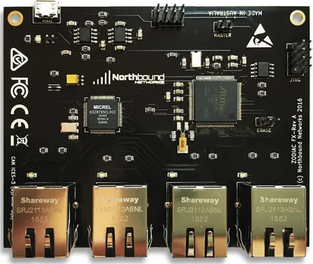
The switches used in this thesis are the Zodiac FX OpenFlow switch, made by Northbound Networks1_{. This is a small four-port switch that supports the OpenFlow protocol. Figure2shows}

the switch hardware overview. It has a firmware that is fully open source and can be changed or updated via its USB port or web-interface. The standard port configuration is one port directly connected to the SDN controller and the other three ports are to be connected to clients. The web-interface is simple and most actions can be done from there. Examples of web-web-interface functions are configuring MAC addresses, VLAN and OpenFlow preferences. The switch has been made mostly for research with open access firmware.

Figure 2: Northbound Networks Zodiac FX switch1_{is a single board switch with four networking}

ports.

1_{Northbound Networks. Zodiac FX. url: https://northboundnetworks.com/products/zodiac-fx (visited on}

4.1.3 Network virtualization

Network virtualization is a method to combine network resources into a single abstract unit. A network hypervisor can then allocate the combined resources to different flows of traffic. Using this technology, virtual networks are able to share the network hardware while still being separate networks. FlowVisor is a network hypervisor and virtualization software, made to act as a layer between OpenFlow hardware and SDN controllers [3]. It is used to slice up the network into different slices that all can use the same hardware in the network, much like VLAN can share a single trunk connection between switches. FlowVisor works like other computer virtualization software, such as VMware and Oracle VirtualBox. These programs allocate different hardware resources to the virtual machines and the same way does FlowVisor allocate networking hardware resources to different SDN controllers. By having slices, networks are also isolated from each other. Different policies can be created for each slice, and these decide what traffic belongs to which slice and the amount of resources that are allocated for the slice. One slice consists of several flow-spaces. These are defined by the information of the packet header or/and the ingress port. Each flow-space has a rule associated with it, much like a firewall, where the action can be either allow, deny or read-only. These actions restrict or permits the SDN controller from inserting flow entries in the networking hardware. Allow permits all OpenFlow messages, deny drops all messages and read-only allows the message to reach the controller but not change the flow tables in the networking hardware [3]. Figure3shows how OpenFlow requests are directed by the policies.

Figure 3: FlowVisor compares packets to the defined slices in the hypervisor, then rewrites and forwards the OpenFlow message to the correct slice controller [3].

4.1.4 Floodlight SDN controller

The Floodlight controller2 is a widely used enterprise level controller developed by a community and Big Switch Networks. It is issued under the Apache-license and can be used for all OpenFlow requests. It works by acting as a gateway to different applications that run as separate modules. There are a number of modules that comes with Floodlight, such as the Forwarding module that is used in this thesis, but also other modules such as the Learning switch, Load balancer and Firewall. Modules can be configured separately and make decisions based on different fields in IP packet headers. New modules can also be written in the same or other languages than Floodlights native Java language, while using the REST API to communicate with Floodlight. By default, Floodlight uses the Forwarding module that replicates basic switching behavior. Figure4illustrates how Floodlight is designed.

Figure 4: The design of Floodlight.

2_{Project Floodlight. Floodlight Controller. url: https://floodlight.atlassian.net/wiki/spaces/}

5

Related Work

The paper by V. Altukhov and E. Chemeritskiy [5], presents a number of different loop-based measuring methods that are used to measure one-way packet delay inside an isolated network. These methods are used without host computers but instead generating packets inside a switching environment and measuring the delay within the closed environment. Then, when entering a multi-hop environment, multiple measurements are done between every two connected switches and then combined to make up the total delay between the two points. Another observation when forwarding packets are whether the slow path or fast path is used. The slow path is when the SDN controller needs to be involved in the forwarding process, and fast path is when flows already have been inserted into the switch and do not need to contact the controller. For service providers, as stated in [10], it is important to monitor their networks to ensure that the service level agreements are upheld and the capabilities of their networks can keep up with demand. Monitoring a network usually gives an extra overhead in management traffic and by best practices, that should be kept below 5% of all traffic on the network. Ways to monitor networks can be to generate traffic and measure throughput, reading flows and wild carded flows or tagging real traffic and use timestamps. In larger networks measuring between two specific points can be difficult because packets may not use the route that is expected, but instead use different routes between each experiment due to switches receiving different flows from the controller. In this thesis, to ensure accurate results there is only one route available to each client in the network. Considering the slow path and fast path, both are used during measurements and both have a different impact on the network and its performance.

In the master thesis by S. Dabkiewicz [6], FlowVisor is tested and evaluated whether it is suitable for production networks. By 2013 FlowVisor was in version 0.8.5 and not as developed as of today at version 1.2. Still, FlowVisor only supports OpenFlow version 1.0 while version 1.6 is out. It was concluded that FlowVisor was not in a state for use in production environments but well suited for research networks where demands for reliability is not as important. The use of FlowVisor itself is very good where it allows multiple networks to use the same hardware and still be separated. It is not expected that, during this thesis, FlowVisor should be ready for production networks, but it is interesting to have virtualization included in the network for research purposes. Having it included could also give better chances for more development of FlowVisor in the future.

According to N. McKeown et al [2], OpenFlow is a good way to let new research hardware and software into a production network. Because OpenFlow allows different brands of hardware and controllers in a network, experiments can be done inside it without interfering with normal traffic. Administrators can easily manage the network to isolate experiments through the controllers. Some examples where shown how OpenFlow can be used in a number of fields such as VLAN tagging, access-control, VoIP and Quality of Service. This shows that SDN has not only a potential to solve many of the practical problems of traditional networking, but can be a new way to make research easier to conduct on running networks than it is today.

O. Salman et al in their paper [9] are testing out different SDN controllers by measuring through-put and latency. The testing is done by using a program called cbench, which is a SDN controller benchmarking application. By continuously sending OpenFlow requests to the controller, the throughput can be measured by counting the amount of responses per second. Latency is mea-sured by sending a packet and waiting for a response. The time it took for the response to arrive is the delay. A lot of controllers where tested but for this thesis the important one is Floodlight. Floodlight has a relatively low throughput compared to other controllers such as MUL, LibFluid and Beacon. However, Floodlight has fairly good values on when it comes to latency, and it has better documentation than many other controllers. For this thesis, Floodlight is chosen because of the ease of setup and good documentation.

J. Alcorn et al have built a portable testbed for SDN research using four Raspberry PIs and Zodiac FX switches. It was made because virtual hardware produces very inconsistent results compared to real hardware, and more powerful devices was too expensive to afford. Larger SDN

projects like GENI is also expensive to join in to. In their paper [4], they test how virtual machines can perform compared to real hardware. To do this they make four virtual machines with different hardware specifications and run several experiments using different SDN controllers and setups. The results are very inconsistent compared to when using real hardware. It is not a comparison between controllers and hardware, but a proof that research becomes much more valuable if done on real instead of virtual hardware.

6

Method

This section will present the method used to perform this thesis. The thesis aims to experimen-tally show the impacts of SDN and network virtualization on delay and overhead compared to conventional networks. The following method is used to obtain the results.

In the first phase, read and review papers and related work in the context of this thesis. In-vestigate similar works and different ways of measuring delay in networks. This phase focuses on finding relevant information on SDN and network virtualization. The next phase aims to create a problem formulation based on the previous studies. The next step is to evaluate the ideas by doing experimental evaluation. To achieve this, a number of topologies are made to perform experiments on. The results of the experiments are then compared to each other and reported.

7

Problem Formulation

Delays in traffic flow transmissions are something that networks struggle to keep as low as possible at all time. The extensive development and usage of traditional networks has proven that it can meet the requirements of delays for production and home networks. OpenFlow on the other hand is still in a research state and the delays of larger networks are still not fully investigated. This thesis attempts to discover the delays in multi-hop network architectures that use OpenFlow. In this regard, the questions can be formulated as follows:

• How do virtual SDN networks perform in a multi-hop architecture?

• What are the impacts of OpenFlow switches compared to conventional switches in a multi-hop architecture?

7.1

Approach

The goal is to answer the question described in Section 7 by collecting and reviewing data on the delays between different clients in a lab network. There are four different topologies that are used for collecting data and each of them have a different design. This includes single-slice SDN, multiple-slice SDN and non SDN topologies. Data is collected by doing experiments on the topologies. How the experiments are done are later explained in Section 8. The program that will make the measurements are explained in Section 7.3, and Section 7.2 describes the topologies that will be used when doing the experiments. For the configuration commands and files, see Appendix

C. The following equipment are used for the experiments: • 1 Lenovo X220i laptop

• 1 Cisco 2960 switch • 2 Zodiac FX switches

• 4 Raspberry Pi Gen 1 boards

On the laptop there is one virtual machine with one core and 2GB of ram that is running FlowVisor installed. FlowVisor has different configurations for each topology and they are ex-plained in each subsection. Floodlight is running directly on the host and configuration is also specified in each subsection. The Cisco 2960 switch is being used as the hub switch in Topologies 1, 2 and 3.

7.2

Topologies

Following is an explanation of the different topologies and how they are set up and configured. 7.2.1 Topology 1, Single slice SDN

Topology 1 is shown in Figure5 and is a single slice topology that uses two OpenFlow switches and only one SDN controller. This is the most basic multi-hop SDN topology that can be made. The setup is as follows.

On Switch 1, Port 1 is connected to Switch 2. Port 2 is connected to Client A and Port 3 to Client B.

On Switch 2, Port 1 is connected to Switch 1. Port 2 is connected to Client C.

Port 4 on both Switch 1 and Switch 2 are connected to the Hub switch, which is connected to the laptop that runs FlowVisor and Floodlight.

For FlowVisor, one slice is created and named Slice 1. Ports that belong to Slice 1 are Ports 1 to 3 on Switch 1 and Ports 1 and 2 on Switch 2. Floodlight is running on port 10001 with default settings.

7.2.2 Topology 2, Multiple slices SDN with shared port

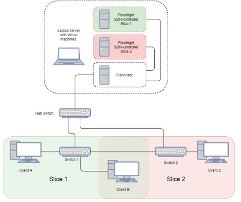
Topology 2 is shown in Figure6, which is similar to Topology 1 except it is partitioned into two slices. Clients A and B belongs to Slice 1, and Client B and C belong to Slice 2. Notice how Client B belong to both slices. In this topology, there are two SDN controllers. Each network slice uses its own controller. The port setup is the same as Topology 1.

For FlowVisor, two slices are created and named Slice 1 and Slice 2. Ports that belong to Slice 1 are Ports 2 and 3 on Switch 1. Ports that belong to Slice 2 are Ports 1 and 3 on Switch 1 and Ports 1 and 2 on Switch 2. Two instances of Floodlight is running simultaneously on the laptop, just with different port configurations. The first instance is connected through port 10001 and the second is connected through port 10002. Both instances are running with the default settings except for the port configuration.

Figure 6: Topology 2 - OpenFlow architecture with two switches and two slices with one shared port.

7.2.3 Topology 3, Multiple slices SDN

Topology 3 is shown in Figure 7 and expands Topology 2 by adding an additional client and removing the shared port that belonged to two slices. Instead one port on each switch belongs to a single slice which is more ideal. The port setup is as follows.

On Switch 1, Port 1 is connected to Switch 2. Port 2 is connected to Client A and Port 3 to Client C.

On Switch 2, Port 1 is connected to Switch 1. Port 2 is connected to Client B and Port 3 to Client D.

Port 4 on both Switch 1 and Switch 2 are connected to the Hub switch, which is connected to the laptop that runs FlowVisor and Floodlight.

Two slices are created in FlowVisor and named Slice 1 and Slice 2. Ports that belong to Slice 1 are Ports 1 and 2 on Switch 1 and Ports 1 and 2 on Switch 2. Ports that belong to Slice 2 are Port 1 and 3 on Switch 1 and Ports 1 and 3 on Switch 2. Floodlight run with the same configuration as in Topology 2.

7.2.4 Topology 4, Cisco only

Topology 4 is shown in Figure8 which only contains Cisco 2960 switches. This is a traditional topology that does not use OpenFlow switches. Experiments on this topology can be compared to the OpenFlow topologies as a reference. The comparison is not completely fair because Cisco is a more powerful hardware than the Zodiac FX. But it can give a general idea of how the overhead is different between the two.

Figure 8: Topology 4 - Traditional architecture using two Cisco 2960 switches.

7.3

Testing program

In order to measure the delays two simple Python programs are used, which are explained in this section.

7.3.1 Sender

The first program is a sender that first makes a time stamp, then sends a message and waits for a response. When it gets the response, it takes another time stamp and subtracts the previous time stamp. This is the round-trip time for the packet. The round-trip time is divided by two in order to get the one-way delay. The program sends a specified number of packages and logs the results for each packet in microseconds in a file. After that it will print out the total time that the test has run for. If a duplicate message is discovered, the program will ignore it and retransmit the latest message to ensure that no packet is skipped. The actual delay when using this specific hardware available is not very interesting, however, in this case we are interested in the delays for different configurations and topologies. The code for this program is available in AppendixA.1.

7.3.2 Responder

The second program is a server that will wait for packets and sends a response whenever it receives a packet. It also checks the content of the message and replies with the same content. This checking is used for identifying duplicate messages. The code for this program is available in AppendixA.2.

8

Experiments

The experiments consist of measuring delays in different topologies and comparing the results. The four topologies that are used in the experiments where described in Section 7.2. Each test consists of sending 10000 packets between two clients. The results are presented in two graphs per test. The first graph consists of the early packets that contains most overhead, and the second shows all packets except the first few packets. This is to see both the impact of the extra delay that the controller request gives, and the performance of continuous messages. Following is a brief description of the experiments.

• Experiment 1, Single slice with SDN: Using Topology 1, measure the delay between Client A to B and A to C. This shows delays when only one slice is configured.

• Experiment 2, Two slice with SDN using shared port: Using Topology 2, measure the delay between Client A to B and B to C. This is the same as the previous experiment but with two slices instead. And shows the difference in delays when using more slices. • Experiment 3, Two slice SDN: Using Topology 3, measure the delay between Client A

to C and B to D. The same as experiment 2 but it does not have any shared port over two slices.

• Experiment 4, Cisco only without SDN: Using Topology 4, measure the delay between Client A to B and A to C. This gives valuable data to compare when not using OpenFlow. • Experiment 5, Fluctuations in SDN: Using Topology 1, measure the delay between

Client A to B. By adding an extra delay between each transmission other results are expected in form of fluctuations shown in earlier experiments.

8.1

Experiment 1, Single slice with SDN

In the first test, the task is to measure the delay between Client A and B. The test took 30047 ms to complete. Figure9 shows that the delay is much bigger during the first packet at around 1500 ms. This is due to the OpenFlow switch that requires to check with the SDN controller about the forwarding rule when a new packet arrives. After the flow is inserted into the switch, Figure10

shows that the packets are being forwarded with less delay. Figure9 shows that the first packet is the one with the highest delay, and in Table 1 the maximum delay is 14.169 ms. The average delay, excluding the early big packets, is around 1.221 ms and the minimum delay is 0.995 ms.

During the experiment some fluctuations are seen in the results. Some peaks are at 6 ms and some at 14 ms. The 14 ms peaks only show up in OpenFlow topologies and the 6 ms peaks are seen in both OpenFlow and non-OpenFlow topologies. The fluctuations appear in a fixed pattern which means that it is not random noise. The way experiments are done also ensures that there are no queues in the switches. This suggests that the 14 ms fluctuations are originating from OpenFlow, and the 6 ms are from the Raspberry Pi or because of general switching behavior. However, ensuring this would need more investigation. Figure11shows some of the 6 ms peaks in Figure9

including packets 1000 to 2500. The 14 ms fluctuations are investigated more in Experiment 5.

Figure 9: E1-A-B - Early packets between client A and B.

Min: 0.995 ms Average: 1.221 ms Max: 14.169 ms Table 1: Values for E1-A-B

Figure 11: Packets 1000 to 2500.

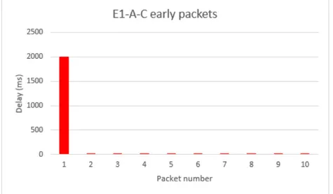
Next is to test delay between client A and C. In this test it is expected to get some extra delay compared to the previous, because the packet must pass one additional switch. The test took 33577 ms to complete and the results are shown in Figure 12 and 13. The first packet has, as before, a larger delay than the other packets because of the switch asking for forwarding rules from the SDN controller. However, the maximum delay is larger compared to the previous test. By comparing the average values, it can be seen that the average delay is increased when the packet is passing two switches instead of one, which is expected.

Figure 13: E1-A-C - Average delays between client A and C.

Min: 1.049 ms Average: 1.356 ms Max: 14.305 ms Table 2: Values for E1-A-C

8.2

Experiment 2, Two slice with SDN using shared port

This experiment uses Topology 2 that has two slices, compared to one slice in Experiment 1. The task is to measure the delay between client A and B. The test took 27499 ms to complete and the results are presented in Figure14and15. In this test the first few packets had a larger delay. This could be due to FlowVisor needing to select a slice for the OpenFlow requests. Table3shows that the average delay is not that different compared to Experiment 2.

Figure 14: E2-A-B - Early packets measurement between client A and B.

Figure 15: E2-A-B - Average delays between client A and B.

Min: 1.004 ms Average: 1.194 ms Max: 14.026 ms Table 3: Values for E2-A-B

The second test is to measure from Client B to C. This test however cannot be completed because there is no connectivity between the two clients. Another test is done measuring from Client C to B instead. This does not work either. By observing the LEDs on the switch, it can be seen that packets travel to Client B but not back to Client C. The port connected to Client B seems to be dropping packets. This is most likely because of FlowVisor not being able to have two slices belonging to the same port.

8.3

Experiment 3, Two slice SDN

During this test, Topology 3 and two slices are used. Compared to the previous experiment, each slice has its own ports and no port is shared. This way there is no unexpected packet drops like in the previous experiment. First is to measure the delay between client A and C. The test took 32967 ms to complete and the results are seen in Figure16and17.

Figure 16: E3-A-C - Early packets measurement between client A and C.

Figure 17: E3-A-C - Average delays between client A and C.

Min: 1.021 ms Average: 1.258 ms Max: 14.225 ms Table 4: Values for E3-A-C

The second test between Client B and D took 33949 ms to complete and the results are shown in Figure18and19. The difference between this and the previous test is that Figure16shows a delay of ˜2600 ms and Figure18have a delay of ˜2000 ms. That is about half a second in difference but there should theoretically be none. This could mean that the overhead is very inconsistent and the two measurements cannot be compared in this fashion. There is an unexpected peak of ˜220 ms around packet number 1100. This is most likely due to a glitch in the transmission. Because it only show up once during all experiments it is very likely just a random occurrence and can be ignored.

Figure 18: E3-B-D - Early packets measurement between client B and D.

Figure 19: E3-B-D - Average delays between client B and D.

Min: 1.083 ms Average: 1.327 ms Max: 216.078 ms Table 5: Values for E3-B-D

8.4

Experiment 4, Cisco only without SDN

In this experiment Topology 4 is used. During the experiment only one Cisco switch is available. To simulate two switches the ports are separated with VLAN tagging. Ports 13-18 are assigned to VLAN 10 and Ports 19-24 are assigned to VLAN 20. Port 13 and 19 are connected together to simulate the connection between two switches. Client A is connected to Port 14 and Client B to Port 15. Client C is connected to Port 20. This setup replicates Topology 4 and during the test it can be seen on the blinking LEDs that traffic is passing through multiple ports as if there were two separate switches.

The first test is between Client A and B and took 25269 ms to complete. It can be seen in Figure20that the first packet does not have that much larger delay than the other packets. This is because the switch does not need to send requests to a controller. Instead it uses ARP requests to find where clients are located, which is a much faster process than talking to an external server.

Figure 20: E4-A-B - Average delays between client A and B.

Min: 0.954 ms Average: 1.141 ms Max: 12.56 ms Table 6: Values for E4-A-B

The second test is between Client A and C. The test took 25822 ms to complete. Results are seen in Figure21and results are as expected about the same as the previous test. Except for the average which is a little bit larger, because the packet is passing through two switches instead of only one.

Figure 21: E4-A-C -Average delays between client A and C.

Min: 0.973 ms Average: 1.168 ms Max: 6.324 ms Table 7: Values for E4-A-C

8.5

Experiment 5, Fluctuations in SDN

The following experiment is to learn more about the 14 ms fluctuations that show up in the OpenFlow related experiments. To do this some extra delay is added between each transmission. The experiment consists of three tests. The first has no delay, the second has a 1 ms delay and the final test has a 10 ms delay. The experiment is based around Topology 1, however, to isolate the cause of the fluctuations all unnecessary hardware is removed. The only hardware used is Client A and B, one OpenFlow switch and the laptop. Switch 1 is directly connected to the laptop instead of the Hub switch.

The first test took 30434 ms to complete and can be seen in Figure22.

The second test is having a short pause of 1 ms between each transmission. It took 135782 ms to complete. Shown by Figure23, there are a lot more fluctuations in this test. However, the peaks are now more spread out between 14 and 9 ms. The 6 ms peaks are also less noticeable.

Figure 23: E5-A-B - Average delays between client A and B with 1 ms delay before each transmis-sion.

The final test have a 10 ms delay between each transmission and took 1033854 ms to complete. The results as seen in Figure24shows a lot more fluctuations than in the previous test. The delay values are also more spread out than before but has a noticeable upper limit of 14 ms.

Figure 24: E5-A-B - Average delays between client A and B with 10 ms delay before each trans-mission.

9

Discussion

Based on the results from the experiments some conclusions can be made. To answer the first question How do virtual SDN networks perform in a multi-hop architecture?

By comparing the average values for all experiments, it can be seen that the average delay for single-hop topologies in Table 1 and 3 is about 1.2 ms, compared to the multi-hops average in Tables 2, 4 and 5 of about 1.3 ms. This result is expected because more hops generate larger delays by default. On the other hand, there are a lot of fluctuations in the delays occurring in all OpenFlow related experiments. These may be a problem when running on a production network where there are time and noise sensitive applications. It is not clear why they occur and more research needs to be done in the area. Now to the overhead. It is determined by the early packets in each test. By comparing the early packet delays in Figure9and14with the values in Figure12,16

and 18, it can be seen that the overhead is increased when moving from a single- to multi-hop topology. It can be assumed that even more hops would generate even larger delays, especially in the first packet. The experiments performed in this thesis only had one packet traversing the network at the time. In a normal production network this is not usually the case and a lot of packet transmissions generate large overheads that can build up a lot of queues in the switches. Considering slices, in Experiment 1 that have one slice only the first packet has a larger delay, however in Experiment 2 and 3 the second packet also have a larger delay. This may be due to having more slices in the network also has an impact on the overhead. And to answer the question. With this particular setup there a lot of overhead and noise. It can be troublesome for SDN to be used in time and noise sensitive or larger networks. But in smaller networks it can work fine as long as the delays are not an issue.

The second question to answer is What are the impacts of OpenFlow switches compared to conventional switches in a multi-hop architecture?

By comparing average values from the SDN single-hop experiments in Table1and3, to the Cisco values in Table6, the average delays are very similar to each other. The Cisco test have about 0.05 ms smaller delay than the SDN experiments. On the other hand, in the multi-hop experiments there is a much bigger difference. Table2,4 and5shows that the average delay is much larger in SDN compared to the Cisco test shown by Table7. It is clear that the OpenFlow switches used in this thesis are slower than the Cisco switch in both single- and multi-hop topologies. This due to the Zodiac FX switch lacking performance to compete with the Cisco switch in general. It is important to keep in mind that the Zodiac FX switch is made for experimental environments only and not production networks. Whereas, the Cisco 2960 is a well-used industry switch that has a lot more power than the Zodiac switch. When looking at the overhead, the Cisco switches have a very small delay, as seen in Figure20and21, compared to the SDN experiments in Figures9,12,14,16

and 18, where the overhead is very large. However, the Cisco switches lacks programmability that SDN have as an advantage. If the overhead could be smaller with more powerful OpenFlow hardware for example, there may be a point at where the two can be better compared in a fair way and the benefits of SDN can show better.

10

Conclusions

This thesis gave a clearer view of how delays and overhead are affected by comparing single- and multi-hop architectures. It can be said that the overhead in this OpenFlow setup is too large to be suitable for time sensitive applications on the network. Other protocols may still work well but with some initial delay. There is also a lot of noise in the transmissions that could have an impact on real-time applications. Virtualization has shown that there is some impact in having multiple slices. Comparing the Cisco switch with the Zodiac switch is not really fair due to the capacity of Cisco switches, however the results showed an overall picture on the delays and overheads due to using OpenFlow switches. In the end, having a centralized control-plane is very valuable for management and scalability purposes.

11

Future Work

There are several directions for future work. One direction is to investigate the reason behind the fluctuation of delays in the OpenFlow switches and if there is a way to decrease the overhead. Moreover, another direction is see if more powerful hardware or other configuration can lower the overhead. Scaling up the network by adding more devices and more realistic traffic patterns is another way to go. It would also be interesting to see the effects when combining wireless and wired networks.

References

[1] B. A. Nunes et al. “A survey of software-defined networking: Past, present, and future of pro-grammable networks”. In: IEEE Communications Surveys & Tutorials 16.3 (2014), pp. 1617– 1634.

[2] N. McKeown et al. “OpenFlow: Enabling Innovation in Campus Networks”. In: ACM SIG-COMM Computer Communication Review. Apr. 2008.

[3] R. Sherwood et al. “Can the Production Network Be the Testbed?” In: OSDI’10 Proceedings of the 9th USENIX conference on Operating systems design and implementation. Oct. 2010, pp. 365–378.

[4] J. Alcorn, S. Melton, and C. E. Chow. “Portable SDN Testbed Prototype”. In: Dependable Systems and Networks Workshop (DSN-W), 2017 47th Annual IEEE/IFIP International Conference. IEEE. 2017, pp. 109–110.

[5] V. Altukhov and E. Chemeritskiy. “On real-time delay monitoring in software-defined net-works”. In: First International Science and Technology Conference (Modern Networking Technologies)(MoNeTeC). IEEE. 2014, pp. 1–6.

[6] S. Dabkiewicz, R. van der Pol, and G. van Malenstein. “OpenFlow network virtualization with FlowVisor”. Master thesis. University of Amsterdam, 2012.

[7] E. Haleplidis et al. Software-Defined Networking (SDN): Layers and Architecture Terminol-ogy. RFC 7426. RFC Editor, Jan. 2015, pp. 1–56.

[8] N. Feamster, J. Rexford, and E. Zegura. “The Road to SDN: An Intellectual History of Programmable Networks”. In: ACM SIGCOMM Computer Communication Review 44 (Apr. 2014), pp. 87–98.

[9] O. Salman et al. “SDN Controllers: A Comparative Study”. In: Electrotechnical Conference (MELECON), 2016 18th Mediterranean. IEEE. 2016, pp. 1–6.

[10] J. Wolfgang and M. Catalin. “Low-overhead packet loss and one-way delay measurements in Service Provider SDN”. In: ONS, Santa Clara (2014).

[11] S. H. Yeganeh, A. Tootoonchian, and Y. Ganjali. “On Scalability of Software-Defined Net-working”. In: IEEE Communications Magazine. Feb. 2013, pp. 136–141.

A

Measuring applications

Following is the code for the two Python applications.

A.1

udp send.py

import socket, time, sys

# Get timestamp function

get_time =lambda: int(round(time.time() * 1000000))

# Set variables REPEATS = 1000 IP = None SAVE = "" try: IP = sys.argv[1] PORT = 5002

REPEATS = int(sys.argv[2]) SAVE = sys.argv[3]

except:

print("Usage: udp_send.py <dest_ip> <repeats> <save_location>") exit()

t = None i = 0 r = []

if not IP or not SAVE: exit() # Set up sockets s = socket.socket(socket.AF_INET, socket.SOCK_DGRAM) s.bind((’0.0.0.0’, 5001)) start = get_time() while i < REPEATS: MESSAGE = "MESSAGE_%i" % i t = get_time()

s.sendto(bytes(MESSAGE, "utf-8"), (IP, PORT)) ANSWER = s.recv(1024).decode() t = (get_time() - t) / 2 r.append(int(t)) if MESSAGE == ANSWER: i += 1 time.sleep(0.01)

print("Finished in: %is" % ((get_time() - start) / 1000000)) with open(SAVE, ’w’) as f:

for i in r:

f.write(str(i) + "\n")

A.2

udp recieve.py

import socket, sys

# Set variables

try:

IP = sys.argv[1]

except:

exit() PORT = 5001

# Set up socket

s = socket.socket(socket.AF_INET, socket.SOCK_DGRAM) s.bind((’0.0.0.0’, 5002))

# Send respond when getting message

while 1:

MESSAGE = s.recv(1024).decode()

s.sendto(bytes(MESSAGE, "utf-8"), (IP, PORT))

B

Virtual machine

The virtual machine that is installed on the laptop is running Ubuntu 14. This is because it is known to have FlowVisor working on it.

C

Configuration

C.1

Zodiac FX configuration

The Zodiac switches had their firmware upgraded from version 0.81 to 0.82. The MAC ad-dresses where also changed from their original adad-dresses to more simple ones. Switch 1 got 00:00:00:00:00:11 and Switch 2 got 00:00:00:00:00:12. Their original addresses are still on a la-bel on the back. The switches connects to FlowVisor by using port 6633.

C.2

FlowVisor configuration

To generate empty configuration file: sudo -u flowvisor fvconfig generate /etc/flowvisor/config.json Following are the different configuration for each topology.

C.2.1 Topology 1

fvctl -f /dev/null add-slice slice1 tcp:10.0.1.1:10001 admin@slice1 fvctl -f /dev/null add-flowspace s1-p1 00:11 100 in port=1 slice1=7 fvctl -f /dev/null add-flowspace s1-p2 00:11 100 in port=2 slice1=7 fvctl -f /dev/null add-flowspace s1-p3 00:11 100 in port=3 slice1=7 fvctl -f /dev/null add-flowspace s2-p1 00:12 100 in port=1 slice1=7 fvctl -f /dev/null add-flowspace s2-p2 00:12 100 in port=2 slice1=7 fvctl -f /dev/null add-flowspace s2-p3 00:12 100 in port=3 slice1=7 C.2.2 Topology 2

fvctl -f /dev/null add-slice slice1 tcp:10.0.1.1:10001 admin@slice1 fvctl -f /dev/null add-slice slice2 tcp:10.0.1.1:10002 admin@slice2

fvctl -f /dev/null add-flowspace slice1-s1-p2 00:11 100 in port=2 slice1=7\ fvctl -f /dev/null add-flowspace slice1-s1-p3 00:11 100 \

in port=3,nw dst=10.0.0.3/24,nw src=10.0.0.10/24 slice1=

fvctl -f /dev/null add-flowspace slice2-s1-p1 00:11 100 in port=1 slice2=7\ fvctl -f /dev/null add-flowspace slice2-s1-p3 00:11 100 \

in port=3,nw dst=10.0.0.7/24,nw src=10.0.0.10/24 slice2=7

fvctl -f /dev/null add-flowspace slice2-s2-p1 00:12 100 in port=1 slice2=7\ fvctl -f /dev/null add-flowspace slice2-s2-p2 00:12 100 in port=2 slice2=7\

C.2.3 Topology 3

fvctl -f /dev/null add-slice slice1 tcp:10.0.1.1:10001 admin@slice1 fvctl -f /dev/null add-slice slice2 tcp:10.0.1.1:10002 admin@slice2 fvctl -f /dev/null add-flowspace slice1-s1-p1 00:11 100 \

in port=1,nw dst=10.0.0.3/24,nw src=10.0.0.7/24 slice1=7 fvctl -f /dev/null add-flowspace slice1-s2-p1 00:12 100 \

in port=1,nw dst=10.0.0.7/24,nw src=10.0.0.3/24 slice1=7

fvctl -f /dev/null add-flowspace slice1-s1-p2 00:11 100 in port=2 slice1=7 fvctl -f /dev/null add-flowspace slice1-s2-p2 00:12 100 in port=2 slice1=7 fvctl -f /dev/null add-flowspace slice2-s1-p1 00:11 100 \

in port=1,nw dst=10.0.2.11/24,nw src=10.0.2.10/24 slice2=7 fvctl -f /dev/null add-flowspace slice2-s2-p1 00:12 100 \

in port=1,nw dst=10.0.2.10/24,nw src=10.0.2.11/24 slice2=7

fvctl -f /dev/null add-flowspace slice2-s1-p3 00:11 100 in port=3 slice2=7 fvctl -f /dev/null add-flowspace slice2-s2-p3 00:12 100 in port=3 slice2=7

C.3

Floodlight

Floodlight was downloaded and installed via the Arch User Repositories (AUR). url: https://aur.archlinux.org/packages/floodlight/.

After the installation, the configuration was copied from/opt/floodlight/src/main/resources/ floodlightdefault.propertiesto/opt/floodlight/controller1.propertiesand/opt/floodlight/ controller2.properties. Then in the copied files, thenet.floodlightcontroller.core.internal. FloodlightProvider.openFlowPortfield was changed to 10001 for controller1 and 10002 for con-troller2.