School of Innovation, Design and Engineering
Västerås, Sweden
Thesis for the Degree of Master of Science (120 credits) in Computer Science with
specialization in Embedded Systems - DVA503 - 30 credits
Towards Defining Models of Hardware Capacity
and Software Performance for Telecommunication
Applications
Janne Suuronen
jsn15011@student.mdh.se
Supervisor: Jakob Danielsson
Mälardalens University, Västerås, Sweden
Supervisor: Marcus Jägemar,
Ericsson, Stockholm, Sweden
Examiner: Moris Behnam
Mälardalens University, Västerås, Sweden
Abstract
Knowledge of the resource usage of applications and the resource usage capacity of hardware plat-forms is essential when developing a system. The resource usage must not over exceed the capacity of a platform, as it could otherwise fail to meet its real-time constraints due to resource short-ages. Furthermore, it is beneficial from a cost-effectiveness stand-point that a hardware platform is not under-utilised by systems software. This thesis examines two systems aspects: the hardware re-source usage of applications and the rere-source capacity of hardware platforms, defined as the capacity of each resource included in a hardware platform. Both of these systems aspects are investigated and modelled using a black box perspective since the focus is on observing the online usage and capacity. Investigating and modelling these two approaches is a crucial step towards defining and constructing hardware and software models. We evaluate regressive and auto-regressive modelling approaches of modelling CPU, L2 cache and L3 cache usage of applications. The conclusion is that first-order autoregressive and Multivariate Adaptive Regression Splines show promise of being able to model resource usage. The primary limitation of both modelling approaches is their inability to model resource usage when it is highly irregular. The capacity models of CPU, L2 and L3 cache derived by exerting heavy workloads onto a test platform shows to hold against a real-life appli-cation concerning L2 and L3 cache capacity. However, the CPU usage model underestimates the test platform’s capacity since the real-life application over-exceeds the theoretical maximum usage defined by the model.
Acknowledgements
To my supervisors Jakob Danielsson and Marcus Jägemar, I extend my deepest gratitude for your guidance, support, understanding and for sharing your knowledge and expertise with me. You both have gone beyond what one can expect from their thesis supervisors. A special thanks to Jakob for supervising me a second time(firstly during my bachelor’s thesis), it is not an understatement to say your guidance and influence has been paramount for completing both my degrees and for arousing my interest of pursuing a PhD in the future.
During the time I was writing this thesis, I was involved in several volunteer assignments at Mälardalen Student Union/Mälardalens Studentkår. During this period, the organisation had a deal with significant challenges, and many involved had to make sacrifices to keep everything afloat. Each one of you has been an inspiration and your endurance through-out difficult chal-lenges have continuously given me new hope and willingness to continue on.
Specific persons’ presence in my life through-out this thesis has kept me from falling into complete depression due to work-related stress. To each one of you, I owe my mental health and everything this thesis corresponds to.
Thank you!
Jessica Tallbacka - For frequently reminding me to prioritise myself and being supportive when I have wanted to give up and drop everything. You are an incredible inspiration and a role model for leadership.
Josefin Häggström - For continually nagging at me to prioritise my mental health and showing invaluable support through-out this semester.
Anton Roslund - Thanks for being an incredibly supportive friend and congratulations on complet-ing your own master’s thesis.
Marja-Lena Isola & Ari Suuronen, my parents, thanks for understanding that I’ve had to dedicate a lot of time to my thesis and volunteer assignments. Your support means the world to me, and thanks for being there when I needed it the most. I love you.
Table of Contents
1 Introduction 1
2 Background 2
2.1 Black-Box modelling . . . 2
2.1.1 Black-Box Hardware Resource Usage and Capacity Modelling . . . 2
2.2 Cache memory . . . 3
2.3 Cache prefetching . . . 4
2.4 Workload Synthesis . . . 4
2.5 Performance Monitoring Unit . . . 5
2.6 Hardware Capacity Planning . . . 5
3 Related work 5 4 Problem formulation 8 4.1 Research Questions . . . 8
5 Method 9 5.1 Threats to validity . . . 10
6 Modelling system behaviour 11 6.1 Definitions . . . 11
6.2 Regression models . . . 12
6.3 Autoregressive models . . . 15
6.4 Likelihood and Probability . . . 16
6.5 Fitness and model selection . . . 17
6.6 Limitations . . . 20
7 Systems solution 20 7.1 Modelling tool . . . 20
7.2 Workloads . . . 21
7.2.1 CPU-bound workload . . . 22
7.2.2 Pattern-based memory access workload . . . 22
7.2.3 Random access memory workload . . . 23
7.2.4 Blocked matrix multiplication . . . 23
7.3 Reading PMU counters . . . 24
8 Experiment 24 8.1 Environment . . . 24
8.2 Test cases . . . 24
8.2.1 Pattern-based memory read-write test case . . . 25
8.2.2 Integer addition test case . . . 27
8.2.3 Random memory read-write test case . . . 28
8.2.4 Blocked matrix multiplication test case . . . 30
9 Results 31 9.1 Model comparison . . . 31
10 Discussion 39 10.1 Resource usage models . . . 39
10.1.1 Polynomial Regression . . . 39
10.1.2 Regression spline models . . . 39
10.1.3 Autoregressive models . . . 40
10.2 Hardware Platform Capacity models . . . 40
11 Conclusions and future work 42
11.1 Future work . . . 42
References 44 A Results on Intel Core i5-8250U 47 A.1 Resource usage models . . . 47
A.2 Capacity models . . . 51
B Complementary results on Intel core i5-4460 64
List of Figures
1 Research Method Block Diagram . . . 92 Visualised example of a simple regression model . . . 14
3 Arbitrary probability distribution curve . . . 16
4 High-level flow model of our proposed auto-modeller . . . 21
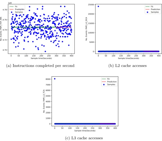
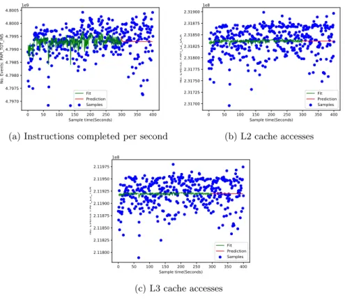
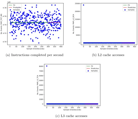
5 AR(1) models of CPU, L2 and L3 cache usage during the pattern-based read-write memory test case . . . 26
6 AR(1) models of CPU, L2 and L3 cache usage during the integer-addition test case 28 7 AR(1) models of CPU, L2 and L3 cache usage during the random memory read-write memory test case . . . 29
8 AR(1) models of CPU, L2 and L3 cache usage during the blocked matrix multipli-cation test case . . . 31
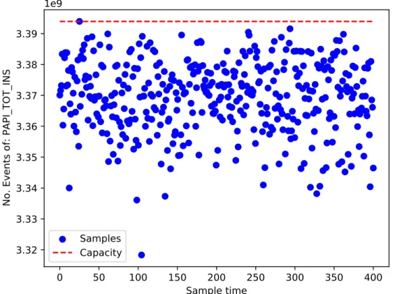
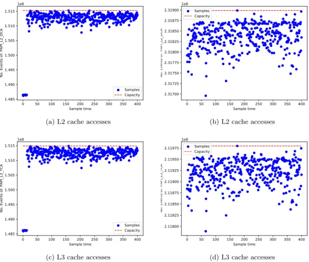
9 CPU capacity model - Intel Core i5-4460 . . . 33
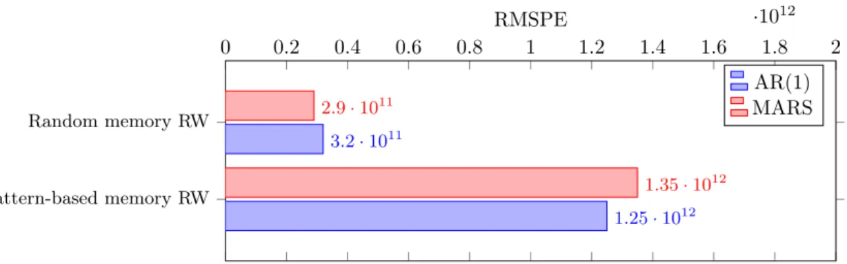
10 RMSPE of AR(1) and MARS(1) models of the integer addition test case . . . 33
11 Maximum L2 and L3 usage - Pattern-based read-write and Random read-write mem-ory test cases . . . 34
12 RMSPEs of AR(1) and MARSRMSPEs of the AR(1) and MARS L2 cache usage models; Pattern-based and random memory read-write test cases . . . 35
13 RMSPEs of AR(1) and MARS L3 cache usage models; Pattern-based and random memory read-write test cases . . . 35
14 RMSPEs of the AR(1) and MARS CPU resource usage model of the blocked matrix multiplication workload. . . 36
15 RMSPE of the L2 and L3 resource usage models; Blocked Matrix Multiplication test case . . . 36
16 MARS resource usage models; pattern-based and random read-write memory test cases - Intel Core i5-4460 . . . 37
17 MARS resource usage models; integer addition and blocked matrix multiplication test cases - Intel Core i5-4460 . . . 38
18 Polynomial regression resource usage models; integer addition and blocked matrix multiplication test cases - Intel Core i5-8250U . . . 52
19 Polynomial regression resource usage models; Pattern-based and random read-write memory test cases - Intel Core i5-8250U . . . 53
20 B-Splines regression resource usage models; Pattern-based and random read-write memory test cases - Intel Core i5-8250U . . . 54
21 B-splines resource usage models; integer addition and blocked matrix multiplication test cases - Intel Core i5-8250U . . . 55
22 N-Splines regression resource usage models; Pattern-based and random read-write memory test cases - Intel Core i5-8250U . . . 56
23 N-splines resource usage models; integer addition and blocked matrix multiplication test cases - Intel Core i5-8250U . . . 57
24 MARS resource usage models; integer addition and blocked matrix multiplication test cases - Intel Core i5-8250U . . . 58
25 MARS resource usage models; integer addition and blocked matrix multiplication test cases - Intel Core i5-8250U . . . 59
26 AR resource usage models; Pattern-based and random read-write memory test cases
- Intel Core i5-8250U . . . 60
27 AR resource usage models; Pattern-based and random read-write memory test cases - Intel Core i5-8250U . . . 61
28 ARMA resource usage models; Pattern-based and random read-write memory test cases - Intel Core i5-8250U . . . 62
29 ARMA resource usage models; integer addition and blocked matrix multiplication test cases - Intel Core i5-8250U . . . 63
30 B-splines regression resource usage models; Pattern-based and random read-write memory test cases - Intel Core i5-4460 . . . 69
31 B-spline resource usage models; integer addition and blocked matrix multiplication test cases - Intel Core i5-4460 . . . 70
32 N-splines regression resource usage models; Pattern-based and random read-write memory test cases - Intel Core i5-4460 . . . 71
33 N-spline resource usage models; integer addition and blocked matrix multiplication test cases - Intel Core i5-4460 . . . 72
34 Polynomial regression resource usage models; Pattern-based and random read-write memory test cases - Intel Core i5-4460 . . . 73
35 Polynomial regression resource usage models; integer addition and blocked matrix multiplication test cases - Intel Core i5-4460 . . . 74
36 ARMA resource usage models; Pattern-based and random read-write memory test cases - Intel Core i5-4460 . . . 75
37 ARMA resource usage models; integer addition test cases - Intel Core i5-4460 . . . 76
List of Tables
1 Examples of workload characteristics . . . 52 Overview of related work . . . 7
3 Properties of the Intel Core i5-4460 processor . . . 25
4 Properties of the Intel Core i5-8250U processor . . . 25
5 Parameters for the pattern-based memory read-write scenario . . . 27
6 Parameters for the integer addition scenario . . . 27
7 Parameters for the random read-write scenario . . . 29
8 Parameters of the blocked matrix multiplication test case . . . 30
9 Maximum CPU usage during the CPU-bound workload test case - Intel Core i5-4460 32 10 Maximum L2 cache usage during the memory-bound workload test cases . . . 33
11 Maximum L3 cache usage during the memory-bound workload test cases . . . 33
12 Capacity model validation outcome . . . 36
13 Model performance metrics during the pattern-based memory read-write - Intel Core i5-8250U . . . 48
14 Model performance metrics during the integer addition test case - Intel Core i5-8250U 49 15 Model performance metrics during the random read-write memory - Intel Core i5-8250U . . . 50
16 Maximum CPU usage during the CPU-bound workload test case - Intel Core i5-8250U 51 17 Maximum L2 cache usage during the memory-bound workload test cases . . . 51
18 Maximum L3 cache usage during the memory-bound workload test cases . . . 51
19 Capacity model validation outcome - Intel Core i5-8250U . . . 51
20 Model performance metrics during the blocked matrix multiplication test case - Intel Core i5-4460 . . . 65
21 Model performance metrics during the pattern-based memory read-write - Intel Core i5-4460 . . . 66
22 Model performance metrics during the integer addition test case - Intel Core i5-4460 67 23 Model performance metrics during the random access read-write memory test case - Intel Core i5-4460 . . . 68
1
Introduction
The telecommunication market suffers from fierce competition, and there is a heavy price-pressure on all telecommunication equipment manufacturers. As a result of the price-pressure, the costs of development and deployment need to decrease. System manufacturers have, traditionally, relied on hardware capacity overcompensation to ensure their applications meet real-time requirements. While the method solves the problem, it is not cost-effective since the hardware is under-utilised. The ideal situation would be to have hardware that can deliver precisely the required capacity. Consequently, avoiding the extra cost of under-utilised hardware and at the same time allowing applications to meet their real-time constraints.
There are two problems to solve if the ideal case is to become a reality. First, the capacity of a hardware platform must be determined. A hardware platform consists of several resources that an application can use to perform work. These resources are finite and are often shared amongst several applications. Therefore, there is a need to understand how much of each resource a platform can provide.
Furthermore, it is of importance to know how resource usage is going to change in the future. It is important since there is a risk that the required capacity for a system is underestimated if we only consider past observations. An underestimation could cause an unexpected negative impact on software performance due to insufficient hardware platform capacity. Thus, we need to model applications’ resource usage and see how it matches the capacity of a hardware platform.
Previous research has investigated several statistical modelling approaches [1–6], such as regressive
and splines models. However, despite that, few [7], at least to our knowledge, have tried to
consolidate hardware resource usage and capacity modelling into the same approach. Effectively, defining a language with that can describe the hardware and software of a system.
Our thesis explores a black box perspective on different approaches to modelling resource usage and capacity. A black box perspective of hardware resources and hardware platforms means that we do not consider the internal properties of the respective object. Sometimes hardware and applications are not fully disclosed and in addition can be large. Therefore, making it difficult and unrealistic to adopt a white-box perspective. Instead, we observe the behaviour of artificial workloads and platforms via hardware performance monitoring units. These units count hardware event occurrences in a platform with which resource usage and capacity can be expressed. The thesis is organised as follows. Section 2 describes the background of our thesis. Section 3 covers state of the art. Our problem formulation is presented in Section 4 and our research method in Section 5. The system context is established in Section 6, and the corresponding system solution is presented in Section 7. The data collection process used to procure training and testing data for evaluated models is explained in Section 8. Section 9 presents and describes our results and Section 10 covers our discussion of said results. Finally, we present our conclusions and suggestions on future work in Section 11.
2
Background
The following subsections provide depth into the areas of black-box modelling; cache memory and its advantages and disadvantages; cache prefetching; workload synthesis. We also cover perfor-mance monitoring units and finalise with describing the notion of hardware capacity planning.
2.1
Black-Box modelling
Constructing a model of a computer system is a way of perceiving its functionality and behaviour. Two types of models are white-box and black-box models.
White-box models focus on describing all the details of a system, thus exposing its internals and
specifications [8], resulting in models with a high level of detail which are ample in cases where
complete insight into a system is required. However, due to their level of detail, constructing white-box models of large and complex systems, for example, those in use by the industry, is
difficult [1,9]. Instead, for these complicated systems, it is more sound to construct a black-box
system model.
By definition, black-box system models disregard of the internals and details of a system and instead focus on the inputs(stimuli) and outputs of the system(response). From the inputs and outputs, the model defers the system’s behaviour, reducing the number of aspects needed to describe it and thus simplifying the model construction process significantly. However, this simplification comes at the cost of more inferior generalisability since black-box models tend to be specific for the scenarios
they represent [1].
2.1.1 Black-Box Hardware Resource Usage and Capacity Modelling
Hardware platforms provide a variety of different resources that applications require in order to complete their tasks. However, these resources can only provide a limited capacity, and sometimes the available capacity is insufficient. The insufficiency problem is even more apparent when multiple applications share the same resources, since they may interfere with each other and thus impact
each other’s performance negatively [10].
A solution to the shared resource contention problem is to measure the usage of shared resources in a system. Doing this can provide with further information about workloads’ non-functional be-haviours, allowing us to construct models of their resource usage. Furthermore, predicting resource
usage enables us to better plan scheduling [10] and determine which capacity is required. Thus,
we can theoretically lower inter-process interference and ensure an acceptable level of performance of applications executing on a platform.
Constructing a white-box model of hardware resource usage of an application can provide beneficial insight into its behaviour. Constructing one would be a complicated task, as it would require full disclosure of an application, something often impossible since commercial application binaries and source code is closed.
A more feasible option is to employ a black-box approach to modelling hardware resource usage. In the context of hardware resource usage stimuli translates to an exerted workload, and usage metrics corresponds to the model’s response.
Another aspect of interest related to hardware resource usage is resource usage capacity. The process of deferring the usage capacity in a black-box model fashion is similar to the one for modelling resource usage. However, the stimuli, in this case, should be a workload that stresses the modelled resource to its boundary. Thus, making the response equivalent to the theoretical capacity of the modelled resource.
2.2
Cache memory
Cache memory, referred to as cache from here-on, is a fundamental hardware component in modern processors, which enables them to retrieve data significantly faster compared to accessing main memory.
Cache typically consists of a faster and expensive underlying memory technology known as Static
Random Access Memory(SRAM) [11]. In contrast to main memory, which is often in an off-chip
location, cache is located on-chip and thus physically closer to the processor compared to main
memory [11]. This shorter distance to the processor and their small sizes the physical access time
to a storage location is kept short.
Architecture and layout
Modern intel-core processors typically implement a 3-level hierarchy, using two local level one
caches, L1-instruction cache and L1-Data cache [12]. These levels denote as 1(L1),
Level-2(L2) and Level-3(L3) cache. Each level of in a cache hierarchy may have its own set of properties that differs from the other levels, such as set-associativity and size. However, there is a general trend for these properties that apply for most Intel processor models.
The L1 cache is the smallest and physically closest to a core and therefore is also the fastest. In multi-core processors, L1 caches are private meaning the belonging core has exclusive ownership of its L1 cache. L2 are larger and local to their relevant core as well. L3 is typically the largest in a cache memory hierarchy and is usually the Last Level Cache(LLC). An additional difference to L3 is that it is shared system-wide.
Each cache level is composed of cache lines, which contains either data or instructions. Each line has an address- and data field and is often either 32 or 64 bytes in size depending on the architecture.
Locality of reference principle
The locality of reference principle states that storage locations in cache memory tend to be
re-accessed in specific assumed patterns. There are two localities, spatial and temporal [11]. Spatial
refers to the assumption that storage locations residing close to a recently accessed one is going to be accessed as well. An example scenario would be the case where data is accessed sequentially. Temporal locality, on the other hand, is the assumption that recently accessed storage locations will be re-accessed again shortly. Typically, this would apply to cases where we loop multiple iterations over a set of storage locations.
Performance issues and benefits
Two metrics commonly used to express cache performance are cache misses and cache hits. A cache miss refers to the case where data requested by an application is not present in cache memory and
must, therefore, be fetched from higher-level caches or main memory [11]. Cache hits are the
opposite of that of cache misses, and more preferable than misses [11].
Caches provide a boost to application performance, but they can also impact it negatively due to certain phenomena. A cause to cache performance issues is the fact that the operating system does not regulate cache usage. Additionally, the way hardware manages cache is also somewhat problematic for application performance. This problem is apparent in situations where multiple applications are executing simultaneously, and are all accessing cache frequently. Hardware man-ages storage locations in cache according to a cache-eviction policy, which dictates how and when cache lines should no longer reside in its respective locations. Hardware makes the call to evict a cache line and application might, therefore, be unknowingly forcing evictions of each other’s data. Furthermore, the usage of cache is unrestricted, which adds to the risk of applications impacting each other’s work as they trigger evictions without knowing who the owner of the stored data is.
2.3
Cache prefetching
Cache prefetching is another technique which significantly speeds up the cache memory manage-ment, which loads either data or instructions ahead of time from, typically, main memory into
cache [14]. The effect of doing is a reduced number of cache misses and thus a smaller impact of
memory latency.
An important aspect to highlight is that prefetching designs can differ between processor models, and therefore, it is a difficult topic to describe generally.
[15] formulate a general description of prefetching as a process performed according to a prefetching
algorithm which covers at least three concerns:
• When to initiate a prefetch • Which line(s) to prefetch
• What replacement(prefetched, referenced or target of a prefetch lookup) status to give the prefetched lines
Cache prefetching happens at either software or hardware level [16]. Software-based prefetching
often means adding prefetch instructions on compiler-level, adding them directly into the source code or during post-compilation analysis.
Hardware-based prefetching uses hardware mechanics to detect access, such as striding, patterns
[16]. A typical such mechanism is stream buffers, which store data and instructions fetched from
the main memory on the order of a prefetch request. The stream buffers themselves are not part of a cache. Instead, they reside and operate independently from the cache hierarchy.
The performance benefits of cache prefetching are noticeable in cases where the prefetchers can derive the memory access patterns used by applications. However, when access to cache is vir-tually random or at least does not follow, for the prefetcher, derivable pattern. Prefetching may become counterproductive and might impact application performance negatively. For example, if a prefetcher retrieves cache lines believing an application is striding through memory with a fixed length but is accessing memory randomly, the prefetched lines will be incorrect, and a miss occurs. In this case, the prefetched lines would be useless as they did not contain the requested data.
2.4
Workload Synthesis
It is crucial to have insight into the performance of a system during the design phase. A way of gauging system performance is to use artificial workloads that stress the system. In cases where system software is unavailable for load testing, synthetic workloads are viable options for
system-benchmarking [17,18]. Thus, workload synthesis can help to determine the suitability of a hardware
platform early [17].
Generation tools require knowledge about the characteristics of the workload to generate similar
workloads. Bagha et al. [19] identify two methodologies for characterising synthetic workloads:
empirical and analytical.
By observing and tracing an existing application, we can synthesise its workload empirically
[17,19,20]. John et al. [20] identified that workloads consist of two different types of
characteris-tics, machine-dependent and machine-independent. Machine-dependent attributes differ between architectures, while machine-independent attributes are general. Table 1 lists examples of each type. Empirically defining a synthetic workload is straight-forward but comes at the cost of gener-alisability and flexibility. The analytical approach uses mathematical models to express workload
characteristics [19]. Each aspect of a mathematical is modifiable, allowing for more flexibility than
Machine-dependent Machine-independent
Cache Hit Ratio Temporal locality of instructions
Cache replacement generated traffic Temporal locality of data
Branch prediction rate Instruction level parallelism
Throughput (operations or transactions/minute) I/O request patterns
Table 1: Machine-dependent(left column) and machine-independent(right column) workload
char-acteristics [19].
2.5
Performance Monitoring Unit
Modern processors often come with hardware devices, known as Performance Monitoring Units(PMU), dedicated to measuring machine-level events. It does this by utilising Performance Counters(PMC) which are interrupt triggered and counts event occurrences on a hardware platform. These events usually are related to either processor or the memory system of a platform. PMCs exist in two different forms, programmable and fixed. However, the availability of each type depends on the platform. Programmable PMCs are configurable to count any event type available in a hardware platform. Fixed PMCs, on the other hand, are locked to counting specific events, such as in case
of the Cortex-A53 model’s PMU, clock cycles [21].
Accessing counters is usually done using APIs, examples are PAPI [22] and Perf [23], which
sim-plifies the usage of the counters. As they otherwise require insight into how to access hardware registers to due to their nature of being part of low-level hardware.
2.6
Hardware Capacity Planning
Ensuring that an application lives up to its expected non-functional requirements requires de-tailed planning of both the application’s parts and the underlying hardware’s ability to deliver the required performance. Likewise, the hardware must not only be able to achieve the desired performance, but provide the needed capacity since hardware resources are finite. So the goal is to determine whether the hardware provides sufficient enough capacity for a given application to meet its non-functional requirements.
Determining the capacity of a hardware platform can be done in several ways.
One method is to formulate capacity using static resource properties, such as cache size and
maximum CPU clock frequency. This kind of information is readily available from hardware
manufactures, and thus is a straight-forward method to employ. However, only considering static properties can be misguiding since we look past potential idiosyncrasies(unexplained hardware design aspects) and online behaviour.
The direct opposite is to measure and determine capacity online. What this refers to is looking at the behaviour and performance a hardware platform delivers during workloads. A technique is to load a system’s resources and measure throughput using hardware counters(Section 2.5). From the measurements, capacity models of the platform’s resources are constructible.
3
Related work
This section presents the state of the art related to this thesis. Table 2 presents an overview of our literature review conducted to constitute this section.
CacheStat [24] is an approach for construction models of cache data locality. The method aims at
devising a probabilistic approach to estimating the cache miss ratio for applications. This is done by discretely sampling references to cache memory and measuring the reuse distance. What the reuse distance refers to is the count of references before a re-access to the concerned address. The
a platform-independent och application agnostic statistical approach for predicting application performance and resource usage.
Lee et al. [26] investigate the use of regressive spline models to predict application performance.
Their approach includes microarchitecture as well as application-specific predictors as their baseline regressive model. Some application-specific predictors considered are cache misses, branch stalls or branch mispredictions. In addition to the baseline model, the authors also compose a set of derivatives. These derivative models focus on different aspects. One variant focuses on stabilising the variance of the predictions. Another variant is transformed to be application-specific. The regressive models achieved a median error of 4.1 per cent for application performance.
Courtois et al. [27] investigate the notion of using Multivariate Adaptive Regression Splines(MARS)
to predict resource usage of applications. The authors conduct their study into MARS models since they argue that simple polynomial models are inadequate for predicting software performance. More specifically, due to their inability to fit against irregular data. The resulting conclusion of the work is that MARS can efficiently estimate parameters of resource functions(functions that define the usage of resource). The authors highlight the benefits of having these kinds of models since they provide crucial information for capacity planning.
Chen et al. [28] and their paper on constructing autoregressive models of resource usage is one of
the few existing papers on the topic, at least to our current knowledge. The purpose of their study is to determine the different phases of software ageing. The authors define resource usage as the average CPU load of a system. The authors evaluate the performance of the general autoregressive model. They also propose a modification of it dubbed Threshold Autoregressive(TAR) model. The TAR model consists of several Autoregressive(AR) parts. Results indicate that the TAR outperforms the general AR model to some extent. However, the AR still achieves a competitive relative quality score, as well as a low error.
[1–5] propose black-box approaches to modelling hardware resource usage and software
perfor-mance. A consideration shared by these works is their view of seeing resource usage as a correlation between a system’s workload and performance metrics. Further, their approaches are empirical as they observe the outgoing performance of a resource to defer the usage. Our thesis employs a similar, somewhat naive and abstracted approach.
A suite of tools that model applications and hardware architectures to evaluate system performance
via co-simulation has been proposed by Pimentel et al [7]. Their work borders ours in the sense that
we wish to evaluate and predict system performance during design space exploration. However, our approach does not employ simulation as means of measuring and quantifying system performance. We do this empirically using hardware performance counters.
[13,22,29–32] use PMU data to identify and remove performance bottlenecks. We intend to use
PMU data as the main input source to our model construction process. Jägemar et al. [10] have
during a previous work, quantified resource usage through PMU counters. We are going to employ the same approach.
Previous work [17,18,20,33–35] on workload synthesis has focused on cloning application
per-formance to generate mimicking workloads. Thus, their [17,18,20,33–35] approaches strive after
replicating select applications’ behaviours and benchmarking system hardware with their synthetic correspondencies. Our also employs workload synthesis. However, we want to employ workload synthesis in a manner where we do not replicate an existing application. Instead, we use it as a means of merely stressing a system to defer its performance attributes. We speculate that our work is easily extendable to cover specific applications.
Li Yin et al.
Performance Models for Storage Systems Black-box Modelling [1]
Podzimek et al. Showstopper: The Partial CPU Load Tool Synthetic Workload Generation [33]
Vogl et al. Using Hardware Performance Events for Instruction-Level Monitoring
on the x86 Architecture Hardware Performance Measurement [29]
Van Ertvelde et al. Workload Reduction and Generation Techniques Synthetic Workload Generation [18]
Bell et al. Improved Automatic Testcase Synthesis for Performance Model Validation Synthetic Workload Generation [34]
Van Ertvelde et al. Benchmark Synthesis for Architecture and Compiler Exploration Synthetic Workload Generation [35]
Azimi et al. Enhancing Operating System Support for Multicore Processors by
Using Hardware Performance Monitoring Hardware Performance Measurement [13]
Cho et al. System-Level Estimation using an On-Chip Bus Performance
Monitoring Unit Hardware Performance Measurement [30]
Li et al. Black-Box Performance Modelling for Solid-State Drives Black-box Modelling [2]
Hatzimihail et al. A Methodology for Detecting Performance Faults in Microprocessors via
Performance Monitoring Hardware Hardware Performance Measurement [31]
Wang et al. Storage Device Performance Prediction with CART Models Black-box Modelling [3]
Dongarra et al. Using PAPI for Hardware Performance Monitoring on Linux Systems Hardware Performance Measurement [22]
Schoonjans et al. On the suitability of black-box performance monitoring for SLA-driven cloud
provisioning scenarios Black-box Modelling [4]
Schneider et al. Online Optimizations Driver by Hardware Performance Monitoring Hardware Performance Measurement [32]
Kim et al. Workload Synthesis: Generating Benchmark Workloads from
Statistical Execution Profile Synthetic Workload Generation [17]
John et al. Workload Characterization: Motivation, Goals and Methodology Synthetic Workload Generation [20]
Eklov et al. A Software Based Profiling Method for
Obtaining Speedup Stacks on Commodity Multi-cores Black-box Modelling [5]
Allam et al. An Efficient CPI Stack Counter Architecture for Superscalar Processors Hardware Performance Measurement [36]
Pimentel et al. The Artemis Workbench for System-level Performance
Evaluation of Embedded Systems Black-box Modelling [7]
Jägemar et al. Enforcing Quality of Service Through Hardware Resource
Aware Process Scheduling Hardware Performance Measurement [10]
Lee et al. Accurate and Efficient Regression Modeling for Microarchitectural Performance and
Power Prediction Black-box modelling [26]
4
Problem formulation
This thesis addresses two problems.
The first problem we wish to solve is how we can model two general system aspects: usage of hardware resources and their capacity. For an application to complete its tasks, it may require different hardware resources, such as CPU or cache memory. How much an application uses of available hardware resources determine the needed capacity for the application to execute optimally. Knowledge of the hardware requirements is paramount when deciding which hardware platform to use in conjunction with an application. Furthermore, it is essential to understand how a program’s resource usage changes for the duration of its execution. This understanding is especially beneficial in a system where multiple applications share resources. As both access to and usage of resources
may be hampered by the number of applications simultaneously executing. However, gaining
this understanding can be tricky just be looking at specifications since hardware platforms and applications might not be fully disclosed.
We aim to tackle this problem by investigating black-box prediction models of hardware resource usage and empirical capacity models. This approach allows us to neglect the specifications and internal of both hardware platforms and applications. Instead, the focus is on quantifying and modelling resource usage and capacity based on observable hardware events. The focus is on the usage of cache memory and CPU cores as these resources are two primary resources often used by applications, in addition to main memory.
The second problem this thesis investigates is how a platform can be determined to be sufficient enough to sustain a known system.
A crucial aspect of designing a functioning system is ensuring that system applications fulfil their non-functional requirements. Fulfilling these requirements depends to some extent on the hardware platform the system is using. The naive approach is to acquire over-powered hardware, and that way ensure applications will meet their non-functional requirements. However, this is not as cost-effective as the platform is under-utilised. Instead, a system designer wishes to find the optimal hardware platform for a given system in terms of utilisation and cost. To make this informed decision, a system designer requires knowledge of applications’ resource usage over time and the capacity of a hardware platform.
Using the solution we devise for our first research problem, we consequently solve the second problem, since we acquire the needed information described previously.
We derive three research questions based on the previous two research problems. Subsection 4.1 lists our research questions.
4.1
Research Questions
RQ1: How can CPU and cache resource capacity and usage be modelled? RQ2: How can software performance be modelled?
RQ3: How can resource capacity and system performance be combined to create a forecast on application behaviour on different systems?
5
Method
This thesis is formulated as an empirical study with deductive reasoning as its research method.
Literature Review
Formulate Research Questions
Construct Hypothesis Models
Perform Experiment
Deductive Reasoning to form Conclusions
Answer Research Questions
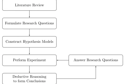
Figure 1: Block diagram of the proposed method The proposed method is presented in Fig. 1.
The initial step of our thesis is to conduct a literature review to establish an overview of the state-of-the-art on the topic of hardware resource usage modelling. This review will, in turn, act as a springboard for our practical solutions to the problems formulated in Section 4. To keep material relevant to related research topics and of high quality, we will search for peer-reviewed and scientific papers in databases and journals on the concerned topics. We present the resulting review in Section 3.
Using the material gathered during the literature review as leverage, we formulate our research questions(Section 4.1). The material will also aid in determining which model types are feasible to include in our study. Once a set of models is selected, we constitute an implementation of the set and empirically validate and test the model types using Commercial Off The Shelf(COTS) hardware. The test and validation procedure consists of four test cases, where we under each test case consider a different workload to produce a varied collection of data sets. This approach contributes to an increased validity as we consider a broad data collection horizon, thus making it easier to draw more generalised conclusions.
The results procured from each test case help us determine the validity of each model type we in-vestigate. Onto which we apply deductive reasoning to answer our research questions qualitatively.
5.1
Threats to validity
Since our study is empirical it is important that we discuss potential validity threats. Feldt
et al. [37] identify four types of threats to validity in empirical computer science studies. The
following paragraphs discuss internal, external, construct and conclusion threats to our study.
Internal Validity threats
When it comes to internal validity threats, some risks might be challenging to deal with. Firstly, since our workload generating tool might not be the only application executing in a system, there is a risk for our results to be impacted and thus misguiding due to, for example, inter-process conflicts. Secondly, the operating system(LINUX) may also play a role in impacting model accuracy since it may be running background tasks which can not be influenced by us. As a consequence, the operating system might, without our knowledge, be impacting model accuracy. Thirdly, since the inner workings of a workload are not exposed as we employ black-box modelling during execution time. We must ensure the compiler for the workload source code does not perform architecture-specific optimisations, as it can have further impacts on model accuracy.
External validity threats
External validity concerns the ability to draw generalised conclusions based on a conducted study. This criterion can be troublesome to satisfy in our case due to several aspects. First, we only consider a subset of all hardware architectures, platforms and workloads for our data collection. This limitation is feasible to over-extend the scope of the thesis, but it is essential to highlight that hardware architectures can differ substantially from each other. Thus, the results procured related to one architecture may very well not apply to others.
Likewise, since applications bind to specific types of hardware resources, some not included in the scope of this thesis, our work may suffer further in terms of generalisability. Furthermore, considering the main downside with a black-box approach to modelling, that they tend to become scenario-specific, there is room to question further the generalisability of our results. However, black-box models are relatively easy to construct since the only necessary component is data. Thus, our work is easy to extend to cover more architectures and workloads, and as such, we negate the threats to generalisability to some extent.
Construct validity threats
A potential issue concerning the construct validity of our thesis is if the workload we exert onto a platform is a bad match for the resource usage we desire to measure. For example, if a workload is CPU-bound, it is a bad match to measure only reads and writes to secondary storage. The situation is not very likely to occur, but it is important to have it in mind, so we do not achieve misguiding results. Therefore, we must have a solid understanding of the workloads we are going to load onto a platform.
Conclusion validity threats
The objects under we observe in our thesis are the models we construct of hardware resource usage and capacity. We construct these models using a black-box approach to hardware resources and workloads. Data on event occurrences is our method of quantifying resource usage and capacity, and we collect during 12 datasets during four test cases. An important aspect to consider given this approach is the potential risk of unknown factors affecting the number of event occurrences, in addition to the ones generated by an exerted workload. For example, an undisclosed hardware component can be accelerating specific instructions, or cache accesses related to prefetching does not count towards the total number of accesses. As such, there is a risk that the conclusions we draw from our data and results might be misguiding.
Consequently, the relationship between the workload and the corresponding resource usage may be incorrect and untrue. Combating this validity issue is somewhat complicated as it requires detailed
insight into a platform, as well as the operating system the platform runs. The steps we take in trying to reduce this issue is the minimise the number of running user-space applications, as well as graphical user interfaces.
6
Modelling system behaviour
The main ideas under investigation in this thesis are resource usage and hardware platform capacity, and how to construct statistical models of these notions. These concepts in themselves refer to several aspects which each require a definition in the context of this thesis to be comprehensible. In this section we discuss the theoretical framework that sets the limits and the focus of our study. Subsection 6.1 states relevant formal definitions and limitations emposed onto our thesis scope. Subsections 6.2 and 6.3 presents the theory of the models we investigate. Subsections 6.4 and 6.5 details processes for modelling fitting and estimation, as well as to perform model selection. The section finishes by stating the limitations we set on modelling system behaviour in subsection 6.6.
6.1
Definitions
A hardware resource is a piece of hardware served to applications via an operating system so the applications can complete tasks. Resource usage of an application is quantifiable using hardware event occurrences related to a specific resource. Furthermore, since we consider resources from a black-box perspective, we only consider the input and output of resource. We denote the workload as input and resource usage as output. Given this, a formal definition of hardware resource usage is as follows:
Definition 6.1. Given usage metrics < m0, ..., mi > such as the number of data and instruction
cache accesses to a given cache level, where i is the number of hardware event types related to the
resource x, we generally define the usage yx of a resource x as
yx=< m0, ..., mi> (1)
Naturally, an application may use several resources available to it, and since we define the usage of a single resource. We can define the overall resource usage by an application’s utilised resources.
Definition 6.2. Given the definition for the usage yxof a single resource x (Definition 6.1). The
overall resource usage R of an application app of n available resources is
Rapp=< y0x, ..., y
n
x > (2)
Formally, constructing a model for resource usage prediction, given Definition 6.1, can be defined
as predicting the future resource usage ˆy using a modelling procedure. The main focus is on how
an application’s resource usage changes over time. Thus, we can model an application’s future resource usage based on its past usage of a resource. Making this definition enables us to limit prediction models to consider time as the independent variable and usage as the dependent variable. A general definition of a resource usage model follows.
Definition 6.3. The predicted future usage ˆyx of a resource x is derived by a model of an
appli-cation’s, app, usage of the resource x over a period of time. Where n is the number of observations of the usage of resource x.
ˆ
yx= model(< yx0, ..., y
n
The number of different modelling procedures applicable to Definition 6.3 is vast. Comparing model types and finding one with low prediction error and adequate fitness is an essential step towards defining well-defined and reliable hardware capacity and software performance models. Subsections 6.2 and 6.3 presents two families of models investigated in this thesis.
Resources are finite and have a maximum usage level, thus we define the formal definition of a resource’s maximum capacity as follows:
Definition 6.4. The capacity of a resource X is equivalent to the maximum possible usage ymax
of X irrespective of time.
Xcap= max(yx) (4)
Definition 6.5. A hardware platform HPxconsists of four homogeneous CPU cores, < CP U0...CP U3>
and three levels of cache cachel1, cachel2and cachel3. The usage of these resources follows
defini-tion 6.1.
HPx=< CP U0, ..., CP U3, cachel1, cachel2, cachel3> (5)
Events associated with a resource can be plentiful and some even irrelevant for the scope of this thesis. Thus, we define the events of interest for the resources stated in definition 6.5 as follows.
Definition 6.6. Usage of CPU, yCP U, is defined as the number of instructions completed per unit
of time t.
yCP U = instructions completedt (6)
Definition 6.7. Usage of cache yicacheis defined as the number of accesses done to a cache level i
per unit of time t.
yicache= number of accessest (7)
With the usage of hardware resources and a platform defined, we can define the capacity of a platform.
Definition 6.8. The capacity of a hardware platform, given Definitions 6.1 through 6.5, HPcap
corresponds to the maximum possible usage of each resource part of HPxirrespective of time.
HPcap= max(y0x, ..., y
i
x) (8)
6.2
Regression models
Regressive analysis is a method often employed for either the purpose of building forecast and predictive models, or for inferring cause-effect relationships between dependent and independent variables. Regressive analysis in itself encompasses a wide variety of methods and different models. Regression models are mathematical and statistical models which model relationships between independent and dependent variables. The following paragraphs explain the different regression models we have used in this thesis.
Simple Linear and Polynomial Regression
The relationship between two variables in the case of simple linear regression corresponds to a, best fit, linear line through a data set. Thus, mathematically the variable relationship is defined as a linear equation(as exemplified in Equation 9) with an error term ε. Since some data sets might have a high variance, it is apparent that a linear solution will not fit all data points. Thus, the goal is often to find a solution that is the best fit against a data set.
ˆ
y = β0+ β1x + ε (9)
y is the predicted dependent variable, while β0 and β1 are the estimated model parameters. x the
singular independent variable considered in simple linear regression. ε is error term corresponding
to the deviation between the observed/estimated value ˆy and the actual value, which the model
tried to estimate. Notice the form of equation 9 and that it is nearly identical to an equation of a straight line.
When data points change non-linearly, a suitable option is to model the data using polynomial regression, where a fit happens using an n-th degree polynomial, as opposed to a linear equation. The same applies to polynomial regression concerning prediction errors; the goal is to find the combination of coefficients which produce the smallest prediction error.
A polynomial regression model takes the form shown in Equation (10), where n is the degree of
the polynomial and ε the error term(deviation between the observed/estimated value ˆy and the
actual value), β0...bn correspond to the model parameters.
ˆ
y = β0+ β1x + β2x2+ β3x3+ ... + βnxn+ ε (10)
In contrast to Equation 9, Equation 10 consists of more estimated terms enabling a polynomial model to assume a different hyper-surface than a straight line, as in the case of simple linear
regression. x...xn are the n dependent variables of a data set, which also determines which order
a polynomial regression models assumes.
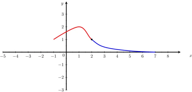
Splines
Despite polynomial regression’s more extensive attention to non-linearity in data, the regression approach might still be insufficient in cases where data vary greatly in select segments. A single polynomial might exclude this variance since it fits to data holistically. A solution is to consider the data set as a composition of smaller segments, referred to as bins, and fitting a polynomial model to each segment. Each segment linked together then forms a spline model for the data which sensitive to changes in the data.
There are three determining factors in the construction of a regression spline model, the degree of freedom and the degree of each segment. The degree of freedom corresponds to the number of segments/bins the data is divided into. Each segment, in turn, can consist of several terms, thus may be linear or polynomial, but every segment is has a fixed number of terms in a spline model. The third factor is the number of points where segments connect with each, so called knots, which is proportional to the number of bins.
yi=
(
β01+ β11xi+ β21x2i + β31x3i + ... + βnxn+ ε if xi< ξ
β02+ β12xi+ β22x2i + β32x3i + ... + βnxn+ ε if xi≥ ξ
(11)
Equation 11 showcases a general simple regression spline model consisting of two segments and one
knot ξ. When xi assumes a value lesser than ξ the first polynomial segment fits against the of xi,
and whenever xi is larger or equal to ξ it is fitted against the second segment. Figure 2 showcases
−5 −4 −3 −2 −1 1 2 3 4 5 6 7 8 −3 −2 −1 1 2 3 0 x y
Figure 2: An arbitrary visualised example of a two segment spline model
A variant of regression spline models is Natural spline.
Natural regression splines extrapolates at boundary values since regression splines tend to be erratic around these areas. Extrapolation at the boundaries means the there are no knots at these points. Thus, the number of knots in a natural spline model is k − 2, where k is the number of knots. The added effect of the extrapolation is that respective boundary is forced to become linear. Effectively reducing the segments beyond the boundaries to assume a degree of one.
Multivariate Adaptive Regression Splines
One issue with regression splines is the fact that non-linearity of data has to be known prior to model construction since they rely on fixed parameters set. The Multivariate Adaptive Regression
Splines(MARS) [26] approach solves the issue by actively searching for select points, knots, in data
and defining a hinge function from one knot to another. Conclusively, the MARS algorithm derives bin sizes on the fly by looking at how data changes in the set. Thus, the number of splines the MARS algorithm builds depends on the frequency of changes in the data.
ˆ f (x) = k X i=1 ciBi(x) (12)
A MARS model is a weighted sum of k basis functions. These basis(Bi(x)) functions take one of
three different forms.
1. A constant, of which there only exists one per model; the intercept term. 2. A hinge function
3. A product of two or more hinge functions
Hinge functions are the vital part of a MARS model since they describe the form of each piece-wise step taken to construct the final model. A hinge functions come in two forms, both presented in equation 13. The constant c is what is known as a knot and x is a variable
The construction process consists of two phases: Forward Pass and Backward pass. During the forward pass phase, we search for the basis functions that achieve the most massive reduction to the sum-of-squared error. A basis function is defined by two terms, a knot and a variable. Thus, in order to add a new basis function to a model, the MARS algorithm has to go through the following steps:
1. Search over all combinations of existing terms
2. Search over all variables to select one for the basis function
3. Search over all values of each variable to select a knot for a new hinge function.
The search in each step is a pseudo-brute force search because the nature of hinge functions allows them to found relatively quickly.
The forward pass tends to generate an overfitted model and to counter this issue, the backwards pass prunes the model generated from the forward pass phase. Pruning refers to removing terms in a model, in this case, the least effective ones and that way combat overfitting.
6.3
Autoregressive models
A class of predictive models which consider previous values, when predicting future ones, are autoregressive models. The name autoregressive thus comes from the fact that the model regresses onto itself. The underlying idea with autoregressive models is the belief that values a variable previously have assumed influences the variable’s future values. This aspect makes autoregressive models attractive in cases where phenomena vary over time. Furthermore, the focus on historical data and its change over time, makes autoregressive models belong in the time series model-family. A typical use case for autoregressive models is the price of goods predictions since the cost of goods tends to be affected by historical price levels.
The downside of autoregressive models is their assumption that factors that affected the historical values of a variable remains unchanged. In cases where the influencing factors, such as the price of raw materials not dipping hard, change, the autoregressive models end up making inaccurate forecasts. This issue is especially problematic when the influencing factors rapidly change, as the prediction error correlates with how much influencing factors have deviated from their original form. Further, since as mentioned, autoregressive models consider the historical values of a variable.
autoregressive model
The general form of an autoregressive(AR) model(Equation 14) is composed of four terms.
ˆ yt= c + p X i=1 βiyˆt−i+ εt (14)
The c is a constant, εtdenoted as the error term(Also referred to as white noise) and βi the model
parameters. ˆytis the prediction made by the model. p denotes the order of the AR model.
Finally, yt−1, which is the value before yt. The number of preceding values considered in
deter-mining ytdefines the order of the autoregressive model. For example, AR(1) would be a first-order
autoregressive model, where each future value depend on only the quantity before while a
Autoregressive Moving Average model
An extension to the Autoregressive(AR) model type is introducing a Moving Average(MA) com-ponent.
An MA model compared to an AR model considers past forecast errors instead of past predicted values, when trying to predict future variable values. Hence, it is not a regressive model of the more common type. As with AR models, the number of past terms included in the prediction of a future one determines the model order. Equation 15 presents the general MA model.
ˆ yt= µ + εt+ q X i=1 θiεt−i (15)
µ is the mean of the data series, θi the model parameters and εt and εt−i the current and prior
prediction error terms. ˆytis the prediction made by the model.
An Autoregressive Moving Average (ARMA) model combines an AR component with an MA component to create a composite model. Each component can be of different orders from each other, annotated as (p,q). Where p is the order of the Autoregressive component and q the order of the Moving Average component.
Equation 16 presents the general form of an ARMA model.
ˆ yt= c + εt+ p X i=1 βiyˆt−i+ q X i=1 θiεt−i (16)
6.4
Likelihood and Probability
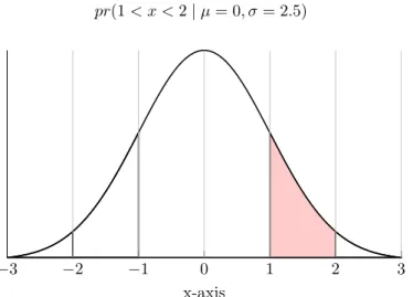
In the context of statistical models, it is essential to highlight the difference between likelihood and probability. Both terms assume the existence of a distribution in a data set. What differs is the interpretation of the distribution. In the case of probability, the distribution curve is fixed, and the area under said distribution is considered the probability. For example, if we wish to determine the probability of a variable assuming a value of between 1 and 2. Given a fixed distribution with a mean(µ) of 0 and a standard deviation(σ) of 2.5. The probability would be mathematically be defined as follows:
pr(1 < x < 2 | µ = 0, σ = 2.5) (17)
−3 −2 −1 0 1 2 3
x-axis
Figure 3: An arbitrary probability distribution curve. The red coloured area corresponds to the probability calculated from equation 17
So the probability is tied to the value range of x we are considering.
Likelihood instead considers a fixed data point and a moving distribution. Continuing with our example of probability, the likelihood of x assuming the value of 1. Given a distribution with a mean(µ) of 0 and a standard deviation(σ) of 2.5, would mathematically be the following:
L(µ = 0, σ = 2.5 | x = 1) (18)
In contrast to probability, likelihood considers how well a distribution will fit the data set since its the influencing term.
Since computing the likelihood is a non-trivial task, it is often common to instead refer to the log-likelihood(Equation 19), which procures the same result but has a significantly more simplified computation.
Building on the example likelihood function in Equation 18, the corresponding logarithmic likeli-hood function is the shown in Equation 19.
log L(µ = 0, σ = 2.5 | x = 1) (19)
The approach to consider the natural logarithm of a likelihood is often preferable in cases where
a sample x consists of n observations x1...xi...xn. The likelihood function of such a sample is the
product of each observation’s likelihood(Equation 20), which is a computationally heavy task. To reduce the number of terms involved in the Equation, we substitute µ and σ with θ.
L(θ | x) = n Y
i=1
L(θ | xi) (20)
By instead working with the log-likelihood(l(θ | x)) the overall likelihood of a sample x consists
of n observations x1...xi...xn is calculate as a sum according to Equation 21. This is substantially
more simple to calculate compared to Equation 20.
l(θ | x) = log n Y i=1 L(θ | xi) = n X i=1 l(θ | xi) (21)
6.5
Fitness and model selection
When evaluating one crucial thing is the fitness of a model. Model fitness tells how well an
estimated model fits against a training data set. Quantifying fitness can be done in several ways. The following paragraphs cover the metrics used through-out this thesis.
Under- and overfitting
Fitted models may exhibit behaviours which promotes a false truth about their accuracy. These behaviours are known as under- and overfitting.
An under-fitted model ignores most data and thus makes a stronger assumption about it. The result is a too simplistic and inflexible model for the considered data set. A not uncommon case of underfitting is fitting a linear model, e.g. a linear regression model, against non-linear data which leads to a portion of data being missed by the model.
Overfitting of a model, on the other hand, occurs whenever a model adapts to a specific data set too well—resulting in a model which fits well against only a specific data set. Meaning it is not
general and therefore does only model a subset of data. A common cause of overfitting is too many parameters in a model, leading to it becoming over flexible. Validating a model often reveals whether a model is over- or underfitting; thus, it is an essential step in any model construction process.
Least Squares and R-squared
Two formulas for determining the prediction error are "Least Squares criterion"(23) and "R-squared" (27).Concretely what it refers to when searching for a line with the least prediction error is finding the coefficients which produce the smallest error term.
The least squares criterion is presented in Equations (22) and (23). The criterion read out is the minimising the sum in Equation (23) which is the sum of the squared differences between actual and predicted values.
ri= yi− f (xi, β) (22) S = n X i=1 ri2 (23)
The R-squared criterion on the other is somewhat more complex compared to the "Least Square". However, it originates from the same starting point, considering the differences between actual and predicted dependent variables. The first step of computing R-squared is summarising the mean of observed data (24) and the actual dependent values, as per Equation (25). Furthermore summarising the residue (Equation (26)), allows the R-squared value for a model to be calculated according to Equation (27). ¯ y = 1 n n X i=1 yi (24) SStot= X i (yi− ¯y)2, (25) SSres= X i (yi− fi)2= X i e2i (26) R2≡ 1 −SSres SStot (27)
In the ideal case, the R2value equals to 1 and equation 26 equals to zero, e.g. there’s no difference
between predicted and actual dependent values.
Information Criterion
In addition to evaluating the quality of model being looking at its fitness, one can consider infor-mation criterion as a measurement of quality of models.
Akaike Information Criteria
The Akaike Information Criteria(AIC) is an estimation of the relative quality of a model, based on
its prediction error [38]. Since AIC measures relative quality, it is a tool usable in model selection,
as the intention is to compare the computed AIC with other models. Thus, determine it is a way of deciding which model represents a data set the best. The formula of AIC is as follows:
AIC = 2k − 2 ln ˆL (28)
where k is the number of estimated parameters in a model. L is the maximum value of theˆ
likelihood function of a model. The constant 2 in-before k is a penalty term which aims at tackling the issue of a model having too many parameters, and thus avoid overfitting.
Corrected Akaike Information Criteria
A problem with AIC is its tendency to overfit models when the size of a sample is small [39], as
it tends to add too many parameters. For the purpose of combating this issue, an modification to AIC exists dubbed Corrected Akaike Information Criteria(AICC). The difference between AIC and AICc is the additional error term for the number of parameters in a model. The definition of AICc follows:
AICc = AIC + 2k
2+ 2k
n − k − 1 (29)
where k corresponds to the number of estimated parameters in a model. AIC the value of a model calculated using 28. n the number of observations in a sample. An additional benefit of the extra penalty term is that as the number of observations n increases, AICc eventually converges to AIC.
Bayesisan Information Criteria
The Bayesian Information Criteria(BIC) [40] is similar to the AIC(Equation 28) with some
ad-ditions, foremost that BIC has a larger penalty term than AIC. The formal definition of BIC follows:
BIC = k ln n − 2 ln ˆL (30)
where k is the number of estimated parameters in a model, n the number of observation in a
considered sample. ˆL is the maximum value of the likelihood function of a model. ln n is key
difference in BIC compared to AIC, the penality term is based on the number of observations in addition to the number of model parameters k.
Hannan-Quinn Information Criteria
In addition to AIC and BIC, another alternative usable for model selection is the Hannan-Quinn Information Criterion(HQIC). Equation 31 gives its definition.
HQIC = −2Lmax+ 2k ln (ln n) (31)
Lmaxcorresponds to the maximum log-likelihood of a model, n the number of observations, and k
Maximum Likelihood Estimation
A probability distribution is defined by two terms: its mean and the standard deviation. These terms also determine the likelihood that a variable will assume a given value in the distribution. Maximising this likelihood is the goal of Maximum Likelihood Estimation. Concretely, this refers to finding σ and µ such that the likelihood of a sample is as high as possible. This description gives us the following equation:
max n X
i=1
l(θ | xi) (32)
MLE is used in the construction of models to find a good fitness of the model to the observed data.
6.6
Limitations
A hardware platform consists of several resources, but this thesis only acknowledges cache memory and CPU cores as the available resources in a platform. Furthermore, we limit ourselves to CPUs with four cores and cache memory with three levels.
In addition we have not considered cases where frequency scaling, effects of temperature or shared resource contention impacts performance or the performance forecast. In other words, our system runs as is; Ubuntu 18.04, without any deliberately enforced bottlenecks.
7
Systems solution
The theoretical context of this thesis is described in Section 6. The following section covers our realisation of the previously mentioned thesis theory.
The description of our theory implementation is split into three parts. First, we describe the modelling tool that can construct regressive and autoregressive forecasting models(Definition 6.3)
of hardware resource usage yxand an application’s usage of them Rapp. Second, we shed the details
of the workloads we used during our data collection as a method to mimic an executing application
on a hardware platform HPx.
7.1
Modelling tool
We implement a model construction tool, which builds regressive and autoregressive models from measured event occurrences. This tool allows us to construct forecasting models(the model function
of Definition 6.3) of resource usage yx and forecasting it to predict ˆyx. In addition to constructing
an overview of the overall resource usage Rappof an application.
The model construction tool is built using Python and produces a forecasting model(Definition 6.3) for each type of event passed to it via a Comma-Separated-Value(CSV) file. That is, it assumes each column in the CSV-file to be one type of hardware event. The tool expects each event type to listed in the header row of a data file.
The tool assumes that sampling happens at a fixed rate over some time, one row corresponding to one measurement. Thus, it does not take direct consideration to the granularity of the sampling frequency. Instead, it is left to the user to interpret what the frequency time-axis pictures. Since some of the regression modelling methods we have implemented rely on static parameters, the tool provides an interactive interface which handles parameter inputs. A prominent case where parameter-tweaking is important is polynomial regression, where the degree of the polynomial is set in before model construction.