2016:01 Literature Study on Sparse Channel Interpretation and Modeling

Research

Literature Study on Sparse Channel

Interpretation and Modeling

2016:01

Authors: Bruno Figueiredo

Chin-Fu Tsang Auli Niemi

SSM perspective

Background

The Swedish Radiation Safety Authority reviews and assesses

applica-tions for geological repositories for nuclear waste. The long term safety

of the repositories depends on the groundwater flow through the rock

surrounding the repositories. Generally, the flow through the

frac-tured rock is calculated by discrete fracture network models (DFN) that

assume flow through the entire fracture planes. However, it is known

that channelling of flow in the fractures may occur and that this can

sig-nificantly influence the results of, for instance, radionuclide transport

calculations. The present report presents a literature study that brings

together information useful for addressing this issue of flow through

sparse channel networks. The broader aim is to improve the knowledge

base for the authority’s evaluation of the long term safety analysis of

license applications for nuclear waste repositories.

Objectives and results

Channelling has been observed in laboratory and field experiments

at various scales. However, it is still an open research issue whether a

sparse channel network is likely to be a better model than the fracture

network model for representing the flow system in fractured rocks. The

present report presents a literature study to bring together information

useful for addressing this issue. Several key questions are discussed,

namely (a) what are the evidences of channelized flow in fractured rocks

with laboratory and field measurements?; (b) what is the relationship

between generalized flow dimensions from well test analysis and sparse

channel network models?; (c) what is the significance of fracture shapes

in hydraulic connectivity?; (d) how does the probability of flow channels

encountering a deposition hole relate to the characteristics of a sparse

channel model?; and (e) are there any specific site studies where sparse

channel models have been used to model the flow and transport in

fractured rocks? A summary, a general discussion and some suggestions

conclude the report.

Need for further research

To increase the knowledge of the effects of channeling on

hydrogeologi-cal modelling in long term safety assessments of nuclear waste

reposi-tories it would be beneficial to conduct studies with a channel network

model to examine implications on results of various field measurements

due to alternative channel sparseness. These field measurements may

include pressure transient testing, borehole logs, tracer tests, cross hole

tests and tunnel wall observations.

Project information

Contact person SSM: Georg Lindgren

Reference: SSM2014-5332

2016:01

1)_{Uppsala University,}

2)_{Lawrence Berkeley National Laboratory, Berkeley, California}

Literature Study on Sparse Channel

Interpretation and Modeling

This report concerns a study which has been conducted for the

Swedish Radiation Safety Authority, SSM. The conclusions and

view-points presented in the report are those of the author/authors and

do not necessarily coincide with those of the SSM.

Contents

Abstract ... 3

1. Introduction ... 4

1.1. Modelling flow and transport in fractured rocks ... 4

1.2. Effect of sorption and matrix diffusion ... 7

1.3. Structure of the report ... 8

2. General concept of channel models ... 10

2.1. The channel network model ... 10

2.2. Sparse channel network ... 13

3. Review of studies addressing some key questions ... 16

3.1. What are the experimental evidence of channelized flow in fractured rocks? ... 16

3.2. What is the relationship between generalized flow dimensions from well test analysis and sparse channel network models? ... 23

3.3. What is the significance of fracture shapes in hydraulic connectivity? ... 25

3.4. How the probability of flow channels encountering a deposition hole relates to the characteristics of a sparse channel model? ... 29

3.5. Are there any specific site studies where sparse channel models have been used to model flow and transport in fractured rocks? ... 30

4. Summary, general discussions and some suggestions ... 33

Abstract

Channelling has been observed in laboratory and field experiments at various scales. However, it is still an open research issue whether a sparse channel network is likely to be a better model than the fracture network model for representing the flow system in fractured rocks. The present report presents a literature study to bring together information useful for addressing this issue. Several key questions are discussed, namely (a) what are the evidences of channelized flow in fractured rocks with laboratory and field measurements?; (b) what is the relationship between generalized flow dimensions from well test analysis and sparse channel network models?; (c) what is the significance of fracture shapes in hydraulic connectivity?; (d) how the probability of flow channels encountering a deposition hole relates to the characteristics of a sparse channel model?; and (e) are there any specific site studies where sparse channel models have been used to model the flow and transport in fractured rocks? A summary, a general discussion and some suggestions conclude the report.

1. Introduction

1.1. Modelling flow and transport in fractured rocks

Flow and transport in fractured rocks at multiple scales continue to be an active area of scientific research (Neuman, 2005; Berkowitz, 2002; Sahimi, 2011) because of on-going activities in several countries as part of their investigation for repositories in fractured rocks deep underground. In particular, Sweden is planning a nuclear waste repository in the municipality of Forsmark (SKB, 2008), whereas in Finland, a nuclear waste repository is planned to be constructed in Olkiluoto (Posiva, 2009 a, b).

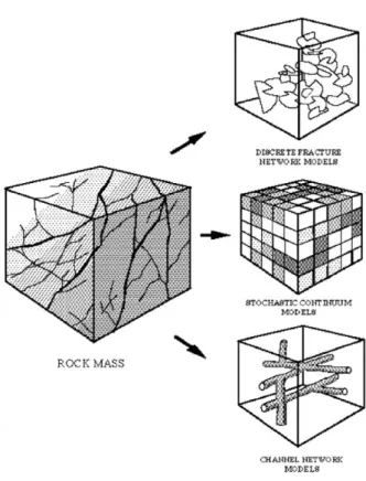
There are a number of issues that need to be addressed when modelling flow and transport in fractured rock under field conditions. These include characterization of the fractures in the rock, as well as model parameterization and upscaling of these parameters, from local small-scale measurements to the scale of repository models. All these issues are complicated by a high level of heterogeneity found in the fractured rock, including that arising from the heterogeneity in individual fractures. Stochastic continuum (SC), discrete fracture network (DFN), and channel network (CN) models (Figure 1) have been developed and used to describe the flow and transport in fractured rocks.

Figure 1: Models to study groundwater flow and solute transport in fractured rocks (Selroos et

In stochastic continuum models (Hartley et al., 2006; Follin, 2008; Neuman et al., 1987; Tsang et al., 1996), the fractured rocks may be represented as an equivalent heterogeneous porous medium with groundwater flow governed by Darcy’s law. The hydraulic conductivity of the equivalent system is treated as a random spatial distribution of block/element hydraulic conductivities that represent the spatially averaged properties over the fractures of the block. This approach is applicable at intermediate and relatively large scales, where effects of individual fractures can be smeared out and represented by properties of the block.

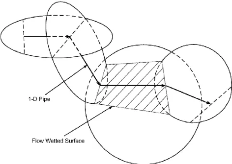
In discrete fracture network models (Long et al., 1982; Cacas et al. 1990 a,b; Joyce et al., 2009; Hartley and Roberts 2012), the groundwater flow and transport in fractured rocks are assumed to occur primarily within fractures. The resulting fracture networks are converted to three-dimensional networks of essentially one-dimensional pipes (Figure 2). Fracture networks are thus mostly modelled as consisting of fully open fractures that intersect each other forming the conductive network. Each fracture is assigned with a volume, size and transmissivity and may be simulated as deterministic or stochastic (Dershowitz and Fidelibus, 1999). Deterministic representations are used when the location, extent, and orientation of particular fractures are well defined from data. Stochastic representations of fractures are most often based on statistical parameters rather than detailed geometric data. The equations representing the flow and transport in the interconnected fracture system are then solved, but the scale of the network simulations is typically limited due to computational constraints. Theoretical and computation approaches are described by Sahimi (2011). An overview of earlier work can be found in Berkowitz (2002).

Figure 2: Discrete fracture network (DFN) conceptual model (Selroos et al., 2002).

One of the main drawbacks of these fracture network models is that they need a large and very detailed data set on fracture orientations, fracture size distributions

translating the field observations to parameters used in the models, and these can be difficult to validate. The field data can be obtained from borehole transmissivity measurements and observations on fracture widths. Calibrations can be made with observations in drifts and tunnels. A considerable number of papers on network modeling are referenced in Neuman (2005) who also gave an overview of the difficulties and intricacies encountered in modeling flow and transport in fractured media (see also Tsang, 2005).

Fracture-scale aperture variability can be included within the fracture-network models (Painter, 2006; Nordqvist et al., 1996), but this further increases

computational demand, thus limiting the scale of model for which computation can reasonably be done. Aperture variability within a fracture causes flow channelling, where the water flow is focused in a few channels with least overall resistance and with the remaining areas of the fracture having practically stagnant water

(Neretnieks, 1993; Tsang and Tsang, 1989; Tsang and Neretnieks, 1998). The so called “flow wetted surface” is defined as the area of the fractures covered by flowing water apart from the fracture areas covered by essentially stagnant water (Moreno and Neretnieks, 1993). In Larsson (2012a, 2013a), the influence of different degrees of heterogeneity in fracture-aperture distributions (as described through their statistical properties) on solute transport is examined and quantified. This influence is studied by first analysing one single fracture, and thereafter applying the results to fracture-network modelling. Larsson et al. (2012b) presents a systematic study of the dependency between fracture aperture statistics and flow wetted surface in strongly heterogeneous fractures. Larsson et al. (2013b) then presents a method to include the effects of fracture aperture variability into the modeling of solute transport in fracture networks.

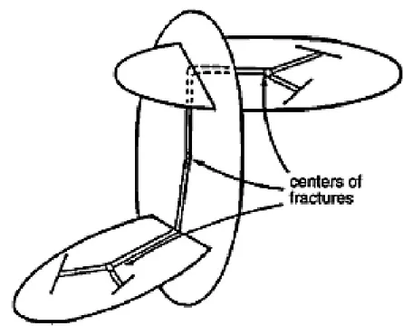
In channel network models (CN), the flow and contaminants are assumed to be distributed among preferential paths in the fracture plane, or channels (Figure 3). These channels may intersect in three-dimensional space, forming a network of channels for the movement and mixing of flowing water. In the channel network model, the equations of flow in each channel are solved via the finite-difference method. Several theoretical studies considering channelized flow in fractured rocks, have been carried out (Rasmuson and Neretnieks, 1986; Neretnieks, 1987; Tsang and Tsang, 1989; Moreno and Tsang, 1994; Moreno et al., 1988, 1990; Tsang et al., 1988; Abelin et al., 1987; Tsang et al., 1991; Moreno and Tsang, 1994; Cacas et al., 1990 a,b; Nordqvist et al., 1992, 1996; Moreno and Neretnieks, 1993; Neretnieks, 1987, 1994; Tsang and Tsang, 1993; Tsang et al., 1996; Black et al., 2006). These studies show that channels in fracture networks can lead to major differences for solute transport characteristics compared to other fracture rock models.

As an important subset of channel network models, the sparse channel network model is characterized by flow in long channels separated from each other by large spacing. However, sets of channels with different orientations can still intersect each other. The sparseness, or the channel spacing being large, can be defined relative to size of the tunnel diameter. More discussion of sparse channel network will be given in the next section.

Figure 3: Conceptual model of a channel network to represent a multiple fracture system

(Cacas et al., 1990b).

1.2. Effect of sorption and matrix diffusion

Different mechanisms are involved for the transportation of solutes in fractured rocks. They include not only the uneven flow distribution, but also interaction between the solutes and the rock. The main interaction mechanisms are sorption and matrix diffusion. An overview of these mechanisms can be found in Retrock (2004). Matrix diffusion is the spread of the solute into the rock matrix, driven by the concentration gradient between solute concentrations in the flowing fluid and in the rock matrix. The solutes may diffuse into and out of the porous rock matrix and the stagnant water and therefore becoming diluted and retarded (Moreno and

Neretnieks, 1993). Sorption is defined as the process in which the contaminant is attached to the surface of a solid phase (Neretnieks, 1993) due to several different causes. For linear sorption, mass adsorbed to the fracture wall is directly

proportional to the excess concentration of solute in the fracture. Rock matrix diffusion and sorption are often lumped together and described by one factor called the “material property group”. The rock may also be altered near the fracture and the fracture surfaces may be covered with different mineral coatings, which will influence the access of solutes to the matrix. These are the important factors involved in the retarding processes that can substantially slow down transport, especially with respect to long time- and large spatial- scale flow, such as that to be evaluated in predictions of potential radionuclide transport into the biosphere, as part of a safety assessment of nuclear repositories (Neretnieks, 1980; Tsang, 2005; Tsang et al., 2008).

Xu et al. (2001) showed that the rock properties display a high heterogeneity in the matrix diffusion coefficient, the effect thereof was further investigated by Zhang et al. (2006). Recent observation has also unveiled an often occurring zone of altered rock at the interface of the fracture and rock matrix, and this altered zone has a higher diffusivity coefficient (Polak et al., 2003; Widestrand et al., 2007). Effective matrix diffusion coefficients are also found to increase with testing scale (Zhou et al., 2007), and Zhang et al. (2006) examined this effect by numerical simulations. These observations have enhanced our knowledge on the heterogeneous nature of fractured rock.

Matrix diffusion from fractures in networks has been modelled and incorporated in transport codes of radionuclide decay chains (Joyce et al., 2009; Hartley and Roberts, 2012). However, these studies are based on the concept that fractures are either open or closed over the entire fracture plane with the consequences that the flowing fractures have to be assumed very sparse and that the rock between and far from the fractures is not readily accessible by diffusion during times of interest. The sparse fractures may lead to poor connectivity of the fracture network and can be sensitive to fracture size distribution as has been pointed out by Berkowitz (2002). The fracture size distribution, assessed mainly from observations on outcrops, has a considerable influence on the connectivity of the fracture network.

It is to be noted that matrix diffusion is handled in fracture network models in a conceptually correct way, especially when fracture aperture variability, is accounted for in the models. In contrast, for stochastic continuum models, matrix diffusion can be calculated as solute exchange between adjacent fast and slow flow lines, which is however an approximation. For channel network models, which represent flow as those in channels, matrix diffusion will be calculated as diffusion radially around channels. Care has to be taken that such calculated diffusion includes diffusion into both the rock and the stagnant water adjacent to the channels.

1.3. Structure of the report

The present report concerns the relevant implications and open issues related to the application of the concept of sparse channel model in the context of sites such as that at Forsmark. This report presents a literature study bringing together

information useful for addressing the questions whether a sparse channel network is likely to be a better representation of the flow system at repository depth and whether this would have any significant impact on the number of deposition holes connected to the flowing network and the magnitudes of the flows to the connected deposition holes. The specific goals of this literature review are firstly to determine if there is scientific information available that can be used to address questions regarding the existence and significance of flow in sparse channel networks; and secondly to analyse what further studies could be conducted to gain more knowledge regarding the nature of the flow system and its effects of flow probability and magnitude into deposition holes emplaced in the fractured systems. The approach used here includes the collection of relevant SKB, Posiva and SSM reports, and key scientific papers, consideration of key issues, discussion of the state of the art, and identification of research needs.

In the face of these objectives, this report is structured in four chapters, of which this introduction is the first one. Chapter 2 entitled General concept of channel models

presents various concepts inherent to the use of channel models for describing the flow and solute transport in fractured rocks. In this chapter, a channel network model which has been applied in the context of the Swedish repository programme for fluid flow and solutes transport calculations is presented. A discussion is made about the necessary model parameters and how they can be best estimated from field and laboratory data.

In Chapter 3, entitled Review of studies addressing some key questions, several questions are discussed, namely:

 what are the evidences of channelized flow in fractured rocks with laboratory and field measurements?

 what is the relationship between generalized flow dimensions from well test analysis and sparse channel network models?

 what is the significance of fracture shapes in hydraulic connectivity?

 how the probability of flow channels encountering a deposition hole relates to the characteristics of a sparse channel model?

 are there any specific site studies where sparse channel models have been used and what are the main findings that were found?

In Chapter 4, a summary and a general discussion are presented together with some suggestions for future work.

2. General concept of channel models

In this section, a general discussion of channel network model will be presented, followed by a discussion of the sparse channel network.

2.1. The channel network model

The channel network model (Moreno and Neretnieks, 1993) has been used to calculate flow and transport of solutes in fractured rocks. The channel network model is a very useful tool that has been applied to site assuming a relatively dense or well-connected channel network system (see section 3.5). However, applications to sparse (or somewhat sparse) channel network have not been done on a systematic way. The code CHAN3D (Gylling et al., 1997, 1999 a,b) is a computational code for the channel network model for the simulation of fluid flow and transport of solutes in fractured rocks. The model assumes that fluid flow takes place in a network of interconnected and randomly generated flow channels in the rock (Figure 4). A flow channel may be formed by a series of individual channel members and it may be connected to, or intercepted by, one, two, three, or even more other channel members. In this code, up to six channels can meet at a grid point (Figure 5).

Figure 5: Fracture planes and channel members (Moreno and Neretnieks, 1993).

The channels can have orientations that are not aligned with a regular rectangular grid. This enables to represent large heterogeneities of the flow distribution

commonly observed and to model solute transport considering advection and matrix diffusion and sorption in the matrix. A hydraulic conductance is assigned to each member of the channel network. The conductance is defined as the ratio between the flow in a channel and the pressure difference between its ends. In applications by Gylling and co-workers, the channel network model is mainly applied not to a sparse network but to a well-connected network. In such cases, the objects such as fracture zones, tunnels, and release sources can be incorporated in the model in a simplified manner by modifying the mean conductance of the channels in these locations. In other words, different values are used for the mean conductance, depending on whether the channel member is located, for example, in a fracture zone or in good rock. Channels located in a fracture zone have larger hydraulic conductivity than if they are in the rock mass. Conductances together with boundary conditions determine the pressures/head field and the flows in the system.

The conductances of the channel members can be assumed to be log-normally distributed, with mean and standard deviation values. The flow is calculated as an electric resistor network problem resolving the distribution of pressure or potential, and the solute transport is calculated by using a particle tracking technique

(Robinson, 1984; Moreno et al., 1988). In the particle tracking technique, many particles are introduced, one by one, into the calculated flow field at one or more locations. Particles arriving at an intersection are distributed in the outlet channel members with a probability proportional to their exit flow rates or according to stream lines. The former is equivalent to assuming total mixing at the intersections and the latter to no-mixing at the intersections. Each individual particle is followed through the network. The residence time for nonsorbing tracers in a given channel is determined by the flow rate through the channel member and its volume. The residence time of an individual particle along its whole path is then calculated as the sum of residence times in all channel members that the particle has traversed. The residence time distribution (RTD) is then obtained from the residence times of a multitude of individual particle runs. The mean and standard deviation values for the residence time may be calculated. When dispersion in the channel and/or diffusion into the rock matrix is also considered, different particles in the same channel member will have a range of residence times. Hence, residence times for the

particles may be described by the residence time distribution of the particles, expressed as a probability density function.

To describe the flow properties of the network the mean channel conductivity and the standard deviation of the channel conductivity are needed. The length

distribution is important when the pressure and flow field are calculated. When the solute transport is simulated, additional channel transport properties are needed. For non-interacting solutes the channel volume is needed. The residence-time

distribution for non-interacting solutes may be calculated and compared to tracer tests in order to test the assumptions of the model. For the simulation of the large-time scale transport of sorbing tracers under repository conditions, it turns out that the volumes of the channels are not a significant factor in calculating of residence time distribution. The channel flow wetted surface (FWS) is however an important parameter for the interacting nuclides that are influenced by sorption and diffusion into and out of the rock matrix and it depends on the channel length and width. Crawford et al. (2002) presents a method for estimating the flow-wetted surface of the rock mass by the observed frequency of open fractures intersecting a borehole between two packers.

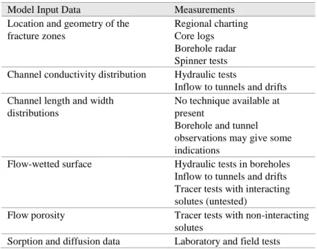
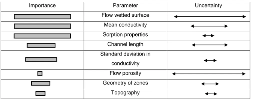
The data needed for the channel model are summarized in Table 1. The values of matrix porosity, effective diffusivity, and sorption constant are needed and they can be determined by laboratory tests. It is more difficult to obtain the data for the fracture zones than for the rock mass. This is because of difficulties in determining, for example, the geometry and hydraulic properties of the fracture zones and their associated variation or range. Table 2 shows an estimate of the importance and uncertainties of various parameters for simulations of fluid flow and solute transport in the channel network model. These estimates and uncertainties were obtained by a qualitative analysis only. To do a quantitative analysis, more research is needed from field and laboratory measurements (Gylling et al., 1999a).

Table 1:Summary of the channel network model input data (Gylling et al., 1999a).

Model Input Data Measurements Location and geometry of the

fracture zones

Regional charting Core logs Borehole radar Spinner tests Channel conductivity distribution Hydraulic tests

Inflow to tunnels and drifts Channel length and width

distributions

No technique available at present

Borehole and tunnel observations may give some indications

Flow-wetted surface Hydraulic tests in boreholes Inflow to tunnels and drifts Tracer tests with interacting solutes (untested)

Flow porosity Tracer tests with non-interacting solutes

Table 2: Importance and uncertainty of different parameters for transport of solutes (Gylling et

al., 1999a).

In order to apply the model to a specific site, additional data such as dip, extension, and width of major fracture zones are needed. The topography and other site characteristic data, such as, the average precipitation that might lead to infiltration, which influences the boundary conditions, are also needed. The geometry for the fracture zones is different from site to site, but parameters like sorption and diffusion properties, on the other hand, may be similar for the same type of rock even if it is obtained from different sites.

2.2. Sparse channel network

Because of the magnitude of the in situ stress component normal to the fractures at depth, the variability of the fractures aperture and the local heterogeneities, it may be possible that many fractures are essentially closed and do not participate in flow and solute transport. In a sparse channel network, flow and transport are assumed to occur in only a few widely spaced 1D channels that are hydraulically active, and the distance between those channels is significant. Figure 6 shows an example of sparse and dense channel networks and Figure 7 shows a discrete fracture model and a sparse channel model of two underground experiments at roughly similar depths in Swedish bedrock.

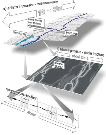
The main characteristics of sparse channel networks are long channels and low numbers of active channels within large volumes of rock (Black 2011a; Geier 2014). Figure 8a is based on the result of interpreting hydrogeological measurements, Figure 8b is an impression based on having examined flow across real fracture surfaces (see also Figure 9), and Figure 8c is channel cross section.

Importance Parameter Uncertainty Flow wetted surface

Mean conductivity Sorption properties Channel length Standard deviation in conductivity Flow porosity Geometry of zones Topography

Figure 6: Examples of sparse (left) and dense (right) channel networks (Black et al., 2007).

Figure 7: Comparison of (a) discrete fracture models and (b) sparse channel model realizations

of similar fractured crystalline rock (Black, 2011a).

When sparse channels interact with underground openings, a “skin” effect is observed. Skin is usually conceived as a region immediately surrounding a borehole or an underground opening whose hydraulic conductivity is different from a wider region. Positive skin effect is associated with a decrease in the value of permeability. Skin is usually evaluated using pressure flow measurements and analysis with Theis solutions, by assessing how far the properties near an underground opening, as indicated by early-time pressure data deviating from theoretical values obtained by assuming that the whole region is homogeneous. Field experiments done in Stripa mine (Sweden) enabled to conclude that inflows to the tunnel are very sparse and converge strongly to the few inflow points available. This is termed

hyper-convergence by Black et al. (2006), who developed a sparse channel network model to model the flow in channel networks towards Stripa Mine. The code HyperConv, developed for this purpose, generates networks of channels on an orthogonal lattice network, applies boundary conditions, calculates flow through the resultant network and ultimately derives values of apparent bulk hydraulic conductivity and skin effect. In contrast to a dense channel model, this sparse channel model was able to

produce the hyper-convergence and the positive skin effects that limit the inflows to the tunnel as were observed.

Figure 8: Schematic of how the sparse channel network at Stripa might appear (a)

multi-fracture plane (b) single multi-fracture plane (c) channel cross-section (Black, 2011a).

The formation of ‘compartments’, in terms of hydraulic head and water chemistry, is a direct consequence of the dominance of a few low conductance links within the network, the ‘chokes’. Thus where there is flow across a region of sparse channels, the measured heads will seem to occur in ‘patches’ of roughly equal head separated by ‘jumps’ of head where flow is occurring through the ‘chokes’. The ‘chokes’ are then the major site of head loss in the system. The large-scale permeability of such systems is largely determined by a few key connections and their values of

conductance (Leung and Zimmerman 2012). In Sawada et al. (2000), in situ tracer migration experiments in fractured granite were carried out which indicated hydraulic compartmentalization and a heterogeneous distribution of conductive fractures.

3. Review of studies addressing some key

questions

In this section, several key questions are discussed: (a) what is the experimental evidence of channelized flow in fractured rocks; (b) what is the relationship between generalized flow dimensions from well test analysis and sparse channel network models; (c) what is the significance of fracture shapes in hydraulic connectivity; (d) how the probability of flow channels encountering a deposition hole relates to the characteristics of a sparse channel model; and (e) are there any specific sites where sparse channel models have been used to model the flow and transport in fracture rocks? The relevant SKB, Posiva and SSM reports, as well as key scientific papers, are referred.

3.1. What is the experimental evidence of channelized

flow in fractured rocks?

Channelling has been observed in laboratory experiments on rock samples with natural or induced fractures on the scale of centimetres to tens of centimetres, and also in field experiments with the scale of meters to 100s of meters. Further, it is observed on walls of drifts and tunnels that water is found to emerge with a channel width of centimetres to tens of centimetres. The data show that the flow-rate distribution is very large among channels. Tsang and Neretnieks (1998) give an overview of the large number of experiments in which channelling has been observed, investigated and interpreted. In this section, the main experimental studies that demonstrate the existence of channelized flow in fractured rocks, are

summarized.

In one of the first field studies, Bourke (1987) selected several fractures in the Cornish granite in England and drilled five boreholes in the plane of a fracture with a length of about 2.5 m. Since the fracture plane undulates to a small extent, the five holes did not lie entirely in the fracture. Water was pressurized in one borehole, and the adjacent holes were divided into 7-cm intervals by the use of packers for measuring the pressure responses at different locations along these boreholes. It was found that many of the packed intervals in the five boreholes did not communicate with each other. Figure 9 shows a sketch of the connected flow pathways inferred from these measurements. The figure shows that the flow areas occupy only about 20% of the fracture surface. This is mainly due to the fracture surfaces not being parallel plates so that the fracture aperture varies over the fracture plane, and water flow takes the easiest pathway from one drill hole to the other, resulting in

channelized flow paths as shown.

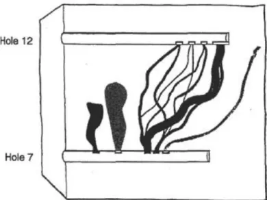
A much more sophisticated and detailed field experiment at a similar scale was performed by Abelin et al. (1988, 1990). In the so-called channelling experiment a fracture in granitic rock was selected in the Stripa iron mine in central Sweden, 360 m below ground level. Two parallel boreholes 1.95 m apart were drilled in the fracture plane. Five different tracers were injected into 5-cm sections of one hole and their emergence in packered intervals in the other, was observed. Results show a tracer transport pattern between the two boreholes (Figure 10), with breakthrough curves at different locations in the observation hole (Figure 11). Breakthrough curves showed multiple peaks and long tails. As pointed out by Tsang and

Neretnieks (1998), the key characteristics of breakthrough curves of tracer transport in channelized flow paths are (a) early and sharp concentration rise of tracer arrival, (b) long tail at large times, and (c) in some of the case, the presence of multiple peaks.

Figure 9: Flow channeling in the plane of a single fracture (Bourke, 1987). The five boreholes

are drilled in the fracture plane. Flow channels are labelled A, B, C and D. Numbers on the histograms are flows from adjacent holes.

Figure 10: Diagram of tracer flow from one borehole (hole 7) to another (hole 12) in the same

fracture plane based on data of responses between packed intervals of the boreholes (Abelin et al., 1990).

Figure 11: Tracer breakthrough curves at various points in the pumping hole 12 (Abelin et al.,

1990).

The Stripa 2D experiment by Abelin et al. (1985) was a larger-scale field experiment than the channelling experiment. Two fractures in granitic rock were identified in one of the tunnels, or drifts, in the Stripa mine. A number of holes were drilled from the drift to intercept these fractures at points 5-10 m above the drift ceiling (Figure 12a). A tracer was deposited at the intersections bracketed by packers emplaced in these holes. The tracer flowed through the fracture plane toward the drift, emerging at the drift along the fracture trace on its ceiling and walls. The emergence of the tracer into the drift was not uniform along the fracture trace; rather, both the flow rate and the tracer concentration were highly variable (Figure 12b).

A further experiment was performed at a different location in the Stripa mine, where a drift intersects a 6-m-wide fracture zone (Birgersson et al., 1993). This zone had a few very prominent flow paths, with the highest flow rate in one out of about 60 collection areas alone accounting for more than 50% of the total flow.

Novakowski et al. (1985) conducted an experiment in a single fracture in a monzonitic gneiss rock body at Chalk River, Ontario, Canada. A pulse of

conservative tracer was injected in a steady dipole flow field using an injection well and a pumping well separated by 10.6 m. The tracer breakthrough curve did not display multiple peaks, and they were able to fit it with a solution of the advective dispersive equation. Another set of five experiments were made in a single fracture in the same rock (Raven et al., 1988) involving both injection-pumping dipole flow field and radial convergent flow field. It was found that the breakthrough curves displayed long tails that could not be fitted by the advective dispersive equation. A much better fit was obtained by considering a "transient solute storage model" that includes a highly mobile flow path and adjacent stagnant or very slow water volumes with tracer exchange between them.

Laboratory tracer tests on natural fractures in granite cores were carried out by Neretnieks et al. (1982) and Moreno et al. (1985). A traced solution was injected at one end of the core and collected at the other. The breakthrough curves were analysed and it was concluded that the water did not flow uniformly through the system but flowed through channels. A model which includes the mechanisms of channelling, surface sorption, matrix diffusion, and matrix sorption, was developed. It was found that the experimental breakthrough curves can be fitted fairly well by this model using independently obtained data on diffusivities and matrix sorption.

Figure 12: (a) Experimental setup of the Stripa 2-D experiment (b) Water and tracer emergence

points along fracture traces in the Stripa 2-D experiment illustrating strong channelization (Abelin et al., 1985).

In the Stripa 3D experiment, a tunnel of about 100 m was constructed, with three boreholes of 75 m in length each drilled into the ceiling of the tunnel (Abelin et al., 1987). Nine high transmissivity intervals were identified in the three boreholes, from which different tracers were injected. The tunnel ceiling and walls were covered by 375 rectangular plastic sheets of 1 m x 2 m in dimension (Figure 13). The tracer

emergence into the tunnel was studied by measuring and analysing the flow into these plastic sheets. In Figure 13 it is seen that the tracers did not emerge uniformly over the whole tunnel surface but rather emerged at much limited locations. Both the flow rates and the tracer concentrations at different locations had a large degree of variability.

Figure 13: (a) Experimental setup for collecting tracer flow in the drift in the Stripa 3-D

experiment. (b) Observations of emergence of flow (dots) and tracers (rectangles) in the drift (Abelin et al., 1987).

Field experiments at a scale of 100 m or more were conducted at the Finnsjön site in Sweden and at the Underground Research Laboratory (URL) in Pinawa, Manitoba, Canada. At the Finnsjön site (Andersson et al., 1988, 1989, 1990), two fracture zones were identified in a granodioritic formation. One of the zones, the

subhorizontal Zone 2, with a thickness of about 100 m located at 100-260 m below the ground surface, was chosen for tracer experiments. Typical behaviour of channelling flow was observed for the breakthrough curves, which displayed a long tail and one or several peaks.

The other large-scale tracer experiments were carried at the URL in Canada (Thompson and Simmons, 1995). At that site three fracture zones were identified in the granitic Lac du Bonnet batholith. In two-well injection-withdrawal tests in one of the fracture zones, multiple peaks were observed in tracer breakthrough curves at short transport distances (about 20 m), while for large transport distances a single well-dispersed peak was obtained (Frost et al., 1992). For tests in another of the fracture zone, tracers were injected in wells in the radially converging groundwater

flow field surrounding the URL shafts and they were collected at groundwater seepage locations in the main and ventilation shafts of the URL. Of the more than 30 breakthrough curves obtained, 12 display multiple peak behaviour, and many have early sharp rise and long tail features, both of which indicate the possible effects of flow channelling.

Large-scale observations in drifts and tunnels have also shown clear effects of channelized flow. At the Final Repository for Reactor Wastes site at Forsmark, more than 14000 m2 of tunnel wall surfaces were surveyed for water effluent spots, and their widths and flow rates were measured. The sparse locations where the water flow emerged in the tunnel and silo system are shown in Figure 14 (Neretnieks, 1994). Measured flow rates are indicated by the length of straight lines at different locations, as shown in Figure 14. Strong variability was found.

Figure 14: Overview of the drifts at the Final Repository for Reactor Wastes, Forsmark

(Neretnieks, 1994). The length of the bars is proportional to the flow rates observed in the drifts.

Abelin et al. (1994) presents channelling experiments that were designed to study the transmissivity and aperture variations in fractures in crystalline rock at a depth comparable to high-level waste repository depths. These experiments were performed in the Stripa mine. Two types of experiments were designed. In the single-hole experiments a hole was drilled > 2 m into the plane of the fracture and injection flow-rates were measured in 5-cm sections using a specially designed injection packer. Photographs were also taken inside the hole along the fracture to determine the visible fracture aperture and to obtain other information such as fracture intersections and fracture infilling. In the double-hole experiment two parallel holes were drilled in the plane of the same fracture at a centre distance of 1.95 m. Hydraulic tests and tracer tests were made between the two holes to obtain information on connections in the plane of the fracture and to obtain information on residence time distributions in different paths (channels) (Figure 15).

Figure 15: Single channels and clusters within a fracture plane (Abelin et al., 1994)

Brown et al. (1998) presents laboratory observations of channel structures in a natural fracture under various flow conditions. A method for obtaining precise replicas of real fracture surfaces using transparent epoxy resins was developed, allowing detailed study of fluid flow paths within a fracture plane. Clear and dyed water were injected into the aperture between fracture surfaces, allowing

examination of the flow field. Digitized optical images were used to observe wetting, saturated flow, and drying of the specimen. Both video imaging and nuclear magnetic resonance imaging techniques showed distinct and strong channelling of the flow at the sub-millimeter to several-centimeter scale (Figure 16). It was found that channels have complex geometries and a wide range of scales. It was found that fluid velocities measured simultaneously at various locations in the fracture plane during steady state flow range over several orders of magnitude, with the maximum velocity a factor of 5 higher than the mean velocity. Due to channelling, then, the breakthrough velocity of contaminants can significantly exceed the mean flow.

Figure 16: (left) Aperture distribution: low to high apertures range from black to white (middle)

Absolute value of the component of volume flow rate parallel to the applied pressure gradient (flow from left to right) (right) Absolute value of the component of volume flow rate perpendicular to the applied pressure gradient (Brown et al., 1998)

To summarize, channelling behaviour is well observed at multiple scales. However, what constitutes sparse channel to be representable by sparse channelling model is not well defined. The “sparseness” depends on scale of observation (sampling scale) or scale of measurement and on the issues to be addressed.

3.2. What is the relationship between generalized flow

dimensions from well test analysis and sparse

channel network models?

Flow dimension refers to the number of space coordinates required to describe flow. In 3D homogeneous media, the flow dimension is expected to be 3. If the flow occurs in a plane, the flow has a dimension of 2. If the flow is along a line, the flow dimension is 1. However, because of heterogeneities, the flow is restricted in space and therefore, the flow can have a fractional dimension smaller than the value for the homogeneous medium, i.e., a dimension that is a fraction smaller than 3, 2 or 1 for the heterogeneous 3D, 2D or 1D space respectively, For the 1D case, the smaller-than-1 dimension occurs if the 1D flow channel reduces in width. Black et al. (1981, 1986) proposes a method for determining the hydrogeological parameters based on a prescribed sinusoidal pressure being applied to an

“excitation” borehole. This test consists of observing the propagation of a pressure perturbation in the formation of interest and interpreting the test by fitting the observations with an idealized flow model. Equations are derived which describe the dependence of pressures and phase lags outside the excitation borehole on distance, signal frequency, specific storage, hydraulic conductivity, and flow rates. These cover two distinct configurations: that of a point source deep within a water-saturated elastic formation and that of a line source totally penetrating a confined aquifer. It was shown that if the fracture density is large and the system is isotropic, then a three-dimensional spherical flow geometry might be considered appropriate. If the fracture density is low or the system is very anisotropic, a one or two-dimensional flow model would probably be preferred.

Barker (1988) presents the generalized radial flow (GRF) model. This model used the flow dimension to describe how the cross-sectional area of flow changes with radial distance from the pumped well. In this approach, the flow dimension may have also non-integer values, but within a framework of average radial flow and homogeneity. There are some difficulties in applying this model: (a) the flow dimension is not a rock property and is likely to be scale dependent, (b) an ideal three-dimensional spherical flow geometry cannot be realized, and (c) anisotropy cannot be included. In addition, the physical interpretation of the flow dimension is unclear, although it is conjectured that the model represents dispersion in a fracture network. This author presents some analytical expressions for the constant rate, constant head and sinusoidal pressure tests.

Doe and Geier (1990) present three complementary methods to determine the geometry and connection between existing fractures from borehole tests. The first method uses the evidence of boundary effects in the well test to determine the distance to and the type of fracture boundary. The second method uses the flow dimension of the borehole test to infer about the fracture system. In the third method, the spacing and transmissivity distribution of individual conductive

were applied to data obtained at 360 m below surface of the Stripa mine (Sweden). It was found that the influence of the boundary effects in the well test results is small. This suggests that the fracture system is well connected, but a significant variation in the spatial dimension of the well tests data was found, ranging from sub-linear (fractures which decrease in conductivity with distance from the hole) to spherical, for three-dimensional fracture systems. Also, it was found that during some pressure tests, the flow dimension changed with time.

In Doe (1991), the generalized dimension approach is applied to the interpretation of constant-pressure well tests. It is shown that the flow dimension cannot be uniquely interpreted because the flow geometry is related with local heterogeneities. This was pointed out as a limitation of the GRF method. Thus, the flow dimension needs to be combined with knowledge provided by geologic, geophysical and hydrologic methods, to construct a reliable model of the fracture network.

In Geier et al. (1996), transient flow data obtained from constant-head injection tests in Äspö Hard Rock Laboratory site were analysed using the GRF model. The analyses provided estimates of flow dimensionality, conductivity, and transmissivity which can be used in the development and validation of conceptual models, and to assess the quality of the existing Äspö conductivity database. Because of low flows indicating tight rock sections, half of the tests in a 3 m packer section and one third on the tests in 30 m section were not interpretable. Results of other interpreted tests showed a flow dimension ranging between 1 (or less) to 3. This author discusses the implications of dimensionality and transmissivity among the main fractures on choosing an appropriate conceptual model.

Walker and Roberts (2003) and Walker et al. (2006) discuss how system geometry and heterogeneities can influence the flow dimension of a fractured rock through analysis of constant-rate hydraulic tests. In Walker and Roberts (2003) it is shown that for a leaky aquifer, the flow dimension is a function of time and leakage factor. For a radial flow system with a linear constant-head boundary, the flow dimension tends to 4 asymptotically. Numerical analysis showed that a stationary

transmissivity field with a modest level of heterogeneity has a stable flow dimension of 2. For a non-stationary field, the flow dimension depends on the form and magnitude of the non-stationarity. In Walker (2006), the flow dimension of stochastic models of heterogeneous transmissivity is determined. Results suggest that the flow dimension may be useful for selecting models of heterogeneity and their parameters.

Kuusela-Lahtinen et al. (2002) apply the general solution for n-dimensional flow obtained by Barker (1988) to study the possibility of using the flow dimension from constant pressure injection tests to characterize the hydraulic conditions of fractured media. Results show a flow dimension of 1 (or less) can be clearly distinguished from a flow dimension larger than 2. But, in many cases, some difficulties were encountered in distinguishing the flow dimension equal to 2, 2.5, and 3 from each other, because of experimental difficulties in achieving the ideal conditions required by the Barker´s solution. In non-unique cases the higher dimensions typically correspond to higher, sometimes unrealistically high, values of specific storage and to the less reliable and less representative early part of the experiment. In this way, most of the observations of a flow dimension equal to 3 can be excluded, leaving the majority observations of the flow dimension equal to 2 and 2.5.

In the work of Kuusela-Lahtinen and Poteri (2010), several data sets provided by constant pressure tests are analysed with the purpose of evaluating the flow

channelling in the scale of a single fracture and the fracture network. The tests have been carried out at the Onkalo site in Finland by using a 2 m test interval

approximately at the depth of the planned repository of the nuclear waste (400 - 450 m). One of the test intervals is intersected by a filled fracture. The flow dimension was found to be 1.5 or 2.0, where the dimension of 2 means that that the flow occurs in the fracture and the dimension of 1.5 may indicate the possibility of narrow flow paths. The other analysed test interval is intersected by three filled fractures. The flow dimension ranged between 2.5 and 3, which implies a behaviour related to a fracture network (homogenous porous media). Flow dimension was also analysed by performing simulated constant pressure tests for different borehole locations over an artificial heterogeneous fracture. The channelling of flow was not demonstrated by the analysis of the flow dimension. Most of the cases showed a similar behaviour that can be represented by a flow dimension of two. Thus, the single-hole testing is probably more sensitive to the connectivity of the fracture network and partitioning of the flow to multiple flow paths through connected fractures than on the

channelization of the flow. Hydraulic single-hole testing activates a limited volume of rock around the tested interval. If the tested volume is mainly limited to the fracture that intersects the borehole, it is more likely to separate channelized from two dimensional flow. If a larger volume of fracture network is activated by the hydraulic test, the transient hydraulic response can be used to distinguish possible channelized flow compared to the cylindrical or spherical pressure field of the test. Follin et al. (2011) studies the discrepancies due to analysis method with or without GRF concept on the results of single-hole transmissivity values in the Forsmark site characterization using data from constant-head injection testing. Data were obtained with two methods: the Pipe String System (PSS method) and difference flow logging with the Posiva Flow Log (PFL method). The analysis showed that the transmissivities derived with standard constant-head injection well test analysis methods and with the GRF concept are similar provided that the dominating flow geometry during the testing is radial. A difference in the results obtained with the PSS and PFL methods were found and it is because the measurements with the PFL method were done after several days of pumping, while the measurements with the PSS method were obtained 20 minutes after test interval perturbation. It is noted that a test interval intersecting a finite “dead-end” fracture or network may produce a flow in the early time period of the PSS test, but record a reduced or no flow by the much later time of running of PFL tool.

To conclude, flow dimension analysis can show effects of heterogeneity that flow is not simple three dimensional or two dimensional. However, its interpretation is ambiguous since the results are also sensitive to flow boundaries and channel intersections, as well as testing time. In the latter, different testing times represent testing of different sizes of rock region around the testing borehole. Thus, when flow dimension analysis shows a simple one dimensional flow over an initial testing period, it can be inferred that channelized flow occurs only over the test volume corresponding to this initial time period.

3.3. What is the significance of fracture shapes in

hydraulic connectivity?

previous review of SKB’s hydrogeological models for Forsmark. They examined how the shape of a transmissive planar feature affected its probability of intersecting other fractures. The evaluation was for two nearby discs and two nearby ellipse of gradually increasing aspect ratio (Figures 17 and 18). This analysis concluded that when equidimensional features cease intersecting, non-equidimensional features continue to intersect even though with a small probability.

According to Black’s work, the intersection of two fractures is not a measure of network performance, whereas continuous connection across the entire network, percolation, is a key indicator. The percolation threshold of ellipses with different values of aspect ratio was estimated by several authors. In Garboczi et al. (1995), analytical predictions were made by using results from lattice models obtained by numerical modelling with ellipsoids of varying aspect ratio. In Robinson (1984), numerical simulations of uniformly distributed square fractures in 3D space were made. De Dreuzy et al. (2000) analyses the intersection of 3D random ellipses with widely scattered distributions of eccentricity and size but within the context of networks with ‘power law’ size distributions.

Figure 19 shows a compilation of the various results. The results presented by Black (2011a, 2012), Garboczi et al., (1995) and Robinson (1984), are consistent with other, and show that as the aspect ratio of the features increases the area per volume density of the network required for percolation decreases. The value of percolation threshold reduces markedly beyond an “aspect ratio” of about 3 or 4. As aspect ratio increases from 1 towards 50 so the feature density required for percolation drops by an order of magnitude. The percolation threshold for the same size of

equidimensional objects lies between 0.15 and 0.5. In order to percolate, disc-shaped fractures require about twice the area density as elliptical fractures of the same area but with a major axis length of about 2 to 3 disc diameters. This shows that equal size discrete fracture network (DFN) models need to have an overestimated density of fractures to percolate and that such DFN models may be a poor representation of reality. In other words, DFN model using fractures with an aspect ratio greater than one are in some cases more realistic. In sparse channel networks, the flow percolates at lower values of area per volume density than networks of equidimensional fractures.

The results presented by De Dreuzy et al. (2000) are also included in Figure 19 and they show that the percolation increases as aspect ratio of the ellipses increases from 1 to about 3, reaches a peak at an “aspect ratio” of 4, and whatever the distributions of length and eccentricity, the values of percolation threshold remain restricted to a range of less than one order of magnitude. This shows almost no dependence of the percolation on the aspect ratio of the ellipses. Black et al. (2007) point out that the results presented by De Dreuzy et al. (2000) look “anomalous and unlikely” and Black (2015) points out some problems with this numerical study.

In Figure 20, the percolation probability as a function of channel length and channel density is presented (Black, 2011a). The channel length is represented by units of sub-channels. The figure shows that using assemblages of 100 realizations, percolation occurred in 100% of cases at lower values of density as channel length increased. The figure shows that the onset of percolation is more abrupt as channel length decreases. This explains why channel networks should be the predominant mechanism for flow in fractured rocks.

Figure 17: Intersection of circular discs and ellipses with different aspect ratio (Black et al.,

2007).

Figure 18: Probability of intersection of two identical ellipses as a function of their scaled

Figure 19: Estimated percolation threshold as a function of aspect ratio (Black, 2011a).

Figure 20: Percolation probability as a function of channel length and channel density (Black,

In Mourzenko et al. (2004), the fracture network permeability is investigated numerically by using a three-dimensional model of plane polygons uniformly distributed in space with sizes following a power-law distribution. The influence of the parameters of the fracture size distribution, such as the power-law exponent and the minimal fracture radius, on the permeability of the fracture network is analysed. In Mourzenko et al. (2005), a numerical study of the influence of the fracture domain size, the flow dimension, and the fracture shape on the percolation threshold of fracture networks, is made. The work reported in these two papers, together with the work reported in De Dreuzy et al. (2000), concluded that the fracture shape is of secondary importance when it comes to hydraulic fracture connectivity.

To summarise the effect of fracture shape on percolation through sparse channel network is likely to be important. The different conclusions from alternative analyses could be due to the different constraints used in the analyses such as power law size distribution and use of different types of calibration data.

3.4. How the probability of flow channels encountering

a deposition hole relates to the characteristics

of a sparse channel model?

The deposition holes can be intersected by fractures with channels of flowing water. The flowrate around a deposition hole and around tunnels control the rate of transfer of corrosive agents and of escaping nuclides to the biosphere. An escaping nuclide will reach the flowing water in the channel and be transported further into the channel network, mixing with water from other channels at some channel intersections or dividing into several outflowing channels at other intersection. Geier (2014) presents an assessment of the SKB’s conceptual model for flow through the fractured rock at Forsmark together with a set of relevant supporting analyses, in response to questions raised by SSM. In this work, four types of models are discussed. Two of these models are DFN models that include heterogeneity in terms of fracture intensity. Possible consequences of using these models include a moderate increase in the number of deposition holes with high flow rate and an increase up to an order of magnitude of the maximum flow rates. Also, a clustering of deposition holes that are subjected to high flow rates, can be obtained. The two other types of models that were discussed include some degree of channelized flow: variable-aperture DFN model and sparse channel network model. A very simplified variable aperture DFN model was also used in a limited assessment in support of Finland's repository programme. The model assumed that the fractures are non-transmissive on randomly distributed patches occupying some specified fraction of its area, with no larger-scale correlations. Results showed an increase of a few percent in the number of deposition holes that are connected to the flowing fracture network. Some discussion was presented on the sparse-channel network model, but it has not been considered in this work to estimate flows to deposition holes in a repository. This type of models was applied only to simulate flow around open tunnels and to explain the so-called “tunnel skin” effects, due to the effects of flow convergence in a sparsely fracture network (Black et al., 2006).

Summarizing, no literature was found on a systematic study of the impact of a sparse channel network on potential flow into deposition holes as a function of sparse channel parameters. Further investigation along this line may be required.

3.5. Are there any specific site studies where sparse

channel models have been used to model flow

and transport in fractured rocks?

Not much work has been done to apply a sparse channel model to study flow and transport in fractured rocks, though "non-sparse” channel models have been applied to analysis of field data. For example, the channel network model (Moreno and Neretnieks, 1993) was used to simulate a long-term pumping and tracer test (LPT2; Gylling et al., 1994, 1998, 1999a) performed at Äspo Rock Laboratory and to predict tracer tests carried out within a 30 m cube scale experiment (Tracer Retention Understanding Experiment-TRUE; Gylling et al., 1999a).

The goal of the LPT2 tests is to investigate the site and to test possible models to be used in safety assessment of a repository. These tests included three major parts: pumping tests, tracer tests, and tracer dilution experiments.

Before the tests, fracture zones were identified and located by surface observations in a preliminary investigation, as well as by geophysical and hydraulic methods. Those zones were confirmed by investigation of the cores from the boreholes and hydraulic head measurements, and they were adjusted with new data during the subsequent excavation of the access tunnel. Several boreholes were drilled to perform the LPT2 experiments. In the pumping experiment, one of these boreholes was used for withdrawal of water and the others were used to monitor the hydraulic head response and some of them also for tracer injection. The pumping test lasted three months and the maximum drawdown in the pumping hole was 51.77 m. When a steady state was reached, the drawdowns were recorded in a great number of sections in the boreholes. The flow rates into the borehole at locations where the hole intersects conducting features were also measured in the experiment. Tracer tests were then initiated with different tracers injected in six borehole sections that showed good connectivity with the withdrawal hole through fractures. The

injections were made for a period of about five weeks. To determine the water flow in the injection sections, tracer dilution experiments were also carried out.

The channel network model used to simulate the LPT2 tests was 1000 m × 700 m × 700 m and included the most of the boreholes in the LPT2 experiment. The

simulation required the knowledge of the geometry of fracture zones and boreholes, the conductance distribution of the channels, flow-wetted surface area, tracer and rock interaction properties, and appropriate boundary conditions. The channel frequency, conductivity distribution and flow-wetted surface were obtained by interpretations of hydraulic packer tests. The mean and standard deviation values of the conductance for channels located in fracture zones were calculated from the analysis of distributions of the transmissivity data taking into account the channel length used in the model and the width of the fracture zones estimated from field data. The flow-wetted surface area was determined through the intersection frequency between boreholes and channels in the rock. The values of the flow porosity, pore porosity and effective diffusivity were not known and were obtained from Stripa data (Birgersson et al., 1992). The channel network model was then used to predict the experiments without calibration to reproduce the field observations. Results of the simulations show that the boundary conditions in the withdrawal hole may play an important role in the calculated drawdown in the measurement

boreholes. The best agreement was obtained when the measured inflows to the withdrawal hole and an infiltration rate condition on the top surface were used as boundary conditions.

The main tracer experiment was in reasonably good agreement, while other tests were overpredicted by the model. The influence of rock interaction was studied by varying the flow-wetted surface and it was found to be a sensitive parameter for the recovery of the tracers.

The tracer tests within the TRUE project were performed at a depth of about 400 m. In the first stage, interference tests, dilution tests, flow loggings, pressure build-up tests, and preliminary tracer tests, were carried out. From the field studies, two fractures (A and B) were identified. Fracture A was found to intersect other fractures. Radially converging tracer tests were performed in this fracture by using nonsorbing tracers with steady-state pumping. In addition, a dipole experiment and tests with sorbing tracers were carried out. Results of these experiments were used to improve the channel network model that was used to predict all these tracer tests. In the modelling, the geometry and boundary conditions were considered and the resulting flow distribution was then used in the transport calculations. This flow model includes a tunnel with the niche, all the boreholes, and fractures A and B. The size of the modelled rock volume was 30 × 30 × 40 m in the longitudinal direction to the tunnel, the horizontal direction, and the vertical direction, respectively. The mean transmissivity values for the different fractures were assigned from the experimental data. In the transport calculation, the solutes were treated as non-sorbing. The tracer transport mechanism in one single channel is by advection together with diffusion into the matrix. The dispersion of the solute occurs because of the heterogeneity of the flow field when the solute is transported with different velocities in the channel network. The tracers were injected as a decaying pulse. From the injection curves and the volumes at the injection points, the injection flow rates and the total injection mass were calculated. Using the available information to calibrate the model, the radial convergent test was well predicted. However, for two of the tests no recovery was obtained over the duration of the experiment, whereas the simulations predicted some loss of tracers but not as much as the experiment showed.

A comparative study of stochastic continuum, discrete fracture network and channel network models to simulate flow and solute transport from the waste canisters to the biosphere was conducted by Selroos et al. (2002). Each approach considers spatial variability of the rock mass via Monte Carlo simulations. To facilitate the

comparison of the results obtained with the three approaches, a common reference case was used, defined by specific model domain and boundary conditions. It was found that the three approaches predict similar values for minimum travel time of the solutes and maximum canister flux, and similar locations for particles exiting the geosphere.

Liu and Neretnieks (2006) integrated the channel network model with a near field model to follow a nuclide from any leaking canister to the effluent points at the ground surface. The channel network model was used to calculate the flow rate in the channels near the deposition holes. By using those flow rates, the near field model was used to calculate the rate of transport of corrosive agents and the release of nuclides from a canister through different pathways into the near field of a repository. Then, the channel network model was used to calculate the paths of the nuclides from the canister through the network by particle tracking.

In Liu et al. (2010), safety assessment calculations for the Forsmark site were performed using a code that couples the channel network model and a near-field model. A site model was developed that includes most of the fracture zones of the

Forsmark site. Deterministic data were used for tunnels, deposition holes, and shafts, while stochastic data were used for existing fractures. The simulations were carried out for 90 different canister locations, which were randomly chosen. The

performance of the simulations was assessed through the F-ratio and the water travel time distributions. The results that were obtained were compared with those

published in Joyce et al. (2009). Although the results cannot be compared directly, a reasonably good agreement was obtained for the F-ratio.

Dershowitz et al. (2002) uses a channel network model and a discrete fracture network model to evaluate flow and solute transport in the Äspö TRUE Block Scale project, Tracer Testing Stage (TTS), at the 50 m to 100 m scale. The fracture network model combines deterministic structures of the hydro-structural model described in Hermanson and Doe (2000) with stochastic fractures (Andersson et al., 2002). Firstly, the hydro-structural model was tested against hydraulic responses and transport parameters derived from conservative tracer transport simulations were obtained. Then, with those parameters, the model was used to predict the sorbing tracer transport experiments. The sorbing tracer breakthrough data obtained by this way was compared with the respective experimental data. The results of this comparison showed that several predicted and measured breakthrough curves agree with each other. For the cases that were not as well matched, additional

supplementary simulations were carried out to derive appropriate sorption

parameters to explain the observed tracer retention. It was found that tracer retention along the tested pathways was greater than predicted.

Dershowitz and Klise (2002) present three studies to simulate tracer tests using the channel network model. These studies were focused on three different aspects of the TRUE Block Scale Hypothesis (Winberg et al., 2000) and addressed key issues regarding (a) transport properties based on conservative and sorbing tracer tests, (b) the possibility of special flow and transport properties at fracture intersection zones (FIZ), and (c) the possibility to improve the hydro-structural model through minor changes in connectivity and transmissivity. It was found that the advection-dispersion-diffusion concept for transport within fracture networks is reasonably consistent with both hydraulic and transport observations and most of the observed hydraulic and transport responses can be explained by the model.

Black (2011b) suggests that most of Borrowdale Volcanic Group (BVG) of the West Cumbrian Coast (WCC) of England, behaves as a sparse or very sparse channel network at depth, and that a proper numerical model should be developed to simulate variable heads and the influence of packer-based test intervals length.