POSSIBILITIES WITH STIRLING
ENGINE AND HIGH TEMPERATURE
THERMAL ENERGY STORAGE IN
MULTI-ENERGY CARRIER SYSTEM
An analysis of key factors influencing techno-economic perspective of
Stirling engine and high-temperature thermal energy storage
MARTIN MYSKA
School of Business, Society and Engineering
Course: Degree project – energy engineering Course code: ERA401
Credits: 30 hp
Program: M.Sc. in Sustainable Energy Systems
Supervisor: Hailong Li Examinor: Eva Thorin Date: 2021-01-11 Email:
ABSTRACT
Small and medium-scale companies are trying to minimise their carbon footprint and improve their cash flow, renewable installations are increasing all over the Europe and are expected to do so in following years. However, their dependency on the weather cause pressure on matching the production with demand. An option how to challenge this problem is by using energy storage. The aim of this project is to determine techno-economic benefits of Stirling engine and high temperature thermal energy storage for installation in energy user system and identify key factors that affect the operation of such system. In order to
determine these factors simulations in Matlab were conducted. The Matlab linear
programming tool Optisolve using dual-simplex algorithm was used. The sensitivity analysis was conducted to test the energy system behaviour. Economic evaluation was done
calculating discounted savings. From the results, it can be seen the significant benefit of SE-HT-TES installation is the increased self-consumption of the electricity from PV installation. While the self-consumption in cases when there was no energy storage implemented was around 67 % and in one case as low as 50 % with the SE-HT-TES the value has increased up to 100 %. Energy cost savings are 4.7 % of the cost for the original data set and go up to 6.2 % when simulation with load shift was executed. Simulations have also shown that energy customer with predictable energy demand pattern can achieve higher savings with the very same system. It was also confirmed that for users whose private renewable production does not match load potential savings are 30 % higher compared to the system where energy load peak is matching the PV production peak. Simulations also shown that the customers located in areas with higher electricity price volatility can benefit from such system greatly.
Keywords: Stirling engine, High-temperature thermal energy storage, Linear optimization, Photovoltaics, Time of Use, Renewable energy, Load shifting, Self-consumption, Power grid
PREFACE
This work was written as a master thesis for a Master of Science in Engineering program at Mälardalen University in Västerås, Sweden in order to investigate Stirling engine and high-temperature thermal energy storage technology and its possibilities of use. The work was conducted from September 2020 to January 2021 under Hailong Li’s supervision from the department of Business, Society and Engineering.
I would like to thank Fredrik Walling for all the help with the master thesis arrangement and provided supervisions. My gratitude goes to Jakub Jurasz for given consultations regarding Matlab programming. Especially thanks to my supervisor Hailong Li for all the support, positive motivation and important advices he provided me through the whole project.
Västerås in January 2021
CONTENT
1 INTRODUCTION ... 1 1.1 Background ... 2 1.2 Purpose ... 2 1.3 Research questions ... 3 1.4 Delimitation ... 3 2 METHOD ... 4 2.1 Model ... 42.2 Net Present Value ... 5
3 LITERATURE STUDY ... 6
3.1 Stirling engine ... 6
3.2 Energy storage ... 8
3.2.1 Thermal energy storage ... 8
3.2.1.1. SENSIBLE HEAT STORAGE ... 9
3.2.1.2. LATENT HEAT STORAGE ... 9
3.2.2 Coupling technology ... 10
3.2.3 Batteries ... 10
3.3 Applications of energy storage ... 11
3.3.1 Load shifting method ... 12
3.3.2 Peak shaving method ... 12
3.4 Solar energy ... 13
4 CURRENT STUDY ... 13
4.1 Load and weather profile ... 14
4.2 Optimization objective ... 15
4.3 Optimisation constraints and boundaries ... 15
4.3.1 Thermal energy storage ... 16
4.3.1.1. HEAT CALCULATION ... 16
4.5 Solar power ... 17
4.6 Operation strategy ... 18
4.7 Simulation scenarios ... 19
4.7.1 Scenario 1, Basic scenario ... 21
4.7.2 Scenario 2, Electricity price ... 21
4.7.3 Scenario 3, Heat price ... 22
4.7.4 Scenario 4, Optimization period ... 22
4.7.5 Scenario 5, Energy demand pattern ... 22
4.7.6 Scenario 6, Energy storage capacity ... 23
5 RESULTS ... 23
5.1 Scenario 1, Basic scenario ... 23
5.2 Scenario 2, Electricity price ... 27
5.3 Scenario 3, Heat price ... 31
5.4 Scenario 4, Optimization period ... 34
5.5 Scenario 5, Shifted load ... 36
5.6 Scenario 6, Different storage capacity ... 38
5.7 Results summary ... 41
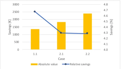
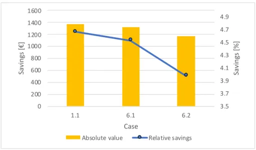
5.7.1 Discounted savings ... 42
6 DISCUSSION ... 42
6.1 Model and methodology ... 42
6.2 Simulation results and economics ... 43
7 CONCLUSIONS ... 46
8 SUGGESTIONS FOR FURTHER WORK ... 47
REFERENCES ... 48
LIST OF FIGURES
Figure 1, Stirling cycle in pV diagram, Source: Mangion et al. (2014) ... 7
Figure 2, Load shifting method applied on 24-hour energy load profile ... 12
Figure 3, Peak shaving method applied on 24-hour energy load profile with maximal reserved power ... 12
Figure 4, Investigated system with implemented PV and SE-HT-TES and with shown electricity and heat flow ... 14
Figure 5, Simulated operation strategy with 24-hour optimization period loop ... 19
Figure 6, Electricity price original (Nord Pool 2019) and increased volatility ... 22
Figure 7, Power demand profile & electricity price (Nord Pool, 2019) ... 23
Figure 8, SOC Thermal energy storage, year ... 24
Figure 9, SOC Thermal energy storage, month ... 25
Figure 10, SOC Battery storage, year ... 25
Figure 11, SOC Battery storage, month ... 26
Figure 12, Annual electricity and heat costs, benchmark ... 26
Figure 13, Thermal energy storage SOC when double electricity price, year ... 27
Figure 14, Thermal energy storage SOC when double electricity price, month ... 28
Figure 15, Thermal energy storage SOC when triple electricity price, year ... 28
Figure 16, Thermal energy storage SOC when triple electricity price, month ... 29
Figure 17, Thermal energy storage SOC when increased electricity price volatility, year ... 29
Figure 18, Thermal energy storage SOC when increased electricity price volatility, month ... 30
Figure 19, Annual savings reached with implemented energy storage, electricity price factor 31 Figure 20, Thermal energy storage SOC when double heat price, year ... 32
Figure 21, Thermal energy storage SOC when double heat price, month ... 32
Figure 22, Thermal energy storage SOC when triple heat price, year ... 33
Figure 23, Thermal energy storage SOC when triple heat price, month ... 33
Figure 24, Annual savings reached with implemented energy storage, heat price factor ... 34
Figure 25, Thermal energy storage SOC with different optimization period, year ... 35
Figure 26, Annual savings reached with implemented energy storage, optimization period factor ... 35
Figure 27, Thermal energy storage SOC with shifted load factor, year ... 36
Figure 28, Thermal energy storage SOC with shifted load factor, month ... 37
Figure 29, Annual savings reached with implemented energy storage system, load profile factor ... 37
Figure 30, Power demand profile & PV production ... 38
Figure 31, Thermal energy storage SOC with storage capacity 600 kWh, year ... 39
Figure 32, Thermal energy storage SOC with storage capacity 600 kWh, month ... 39
Figure 33, Thermal energy storage SOC with storage capacity 400 kWh, year ... 40
Figure 34, Thermal energy storage SOC with storage capacity 400 kWh, month ... 40
Figure 35, Annual savings reached with implemented energy storage, storage capacity factor ... 41
LIST OF TABLES
Table 1, Simulation cases ... 20
Table 2, Simulation input ... 20
Table 3, Basic scenario, technical output ... 24
Table 4, Basic scenario, economic output ... 26
Table 5, Electricity price factor, technical output ... 27
Table 6, Electricity price factor, economic output ... 30
Table 7, Heat price factor, technical output ... 31
Table 8, Heat price factor, economical output ... 33
Table 9, Optimization period factor, technical output ... 34
Table 10, Optimization period factor, economic output ... 35
Table 11, Load profile factor, technical output ... 36
Table 12, Load profile factor, economic output ... 37
Table 13, Energy storage capacity factor, technical output ... 38
Table 14, Energy storage capacity factor, economic output ... 40
Table 15, Discounted savings after 30 years for selected cases ... 42
NOMENCLATURE
Symbol Description Unit
𝐴!" PV module area m2
𝐶#$ Cost for energy €
𝐶%$%&%'( Initial capital cost €
𝐸𝑙)*%+# Electricity price €/kWh
𝐸$ Annual expenses €
𝐺,& Global tilted radiation W/m2
𝐺-. Diffuse horizontal radiation W/m2
𝐺-& Diffuse radiation W/m2
𝐺/. Global horizontal radiation W/m2
𝐺/& Solar radiation W/m2
𝐺*& Reflected radiation W/m2
𝐻𝑒)*%+# Heat price €/kWh
𝑖 Annual interest % p.a.
Symbol Description Unit
𝑁𝑂𝐶𝑇 Nominal operating cell condition °C
𝑃,'&&,+. Battery power charging per hour (p.h.) kWh 𝑃,'&&,-%1 Power from battery discharging p.h. kWh
𝑃23!"# Max. power coupling tech output p.h. kWh
𝑃-#4'$- Power demand per hour kWh
𝑃/*%- Power from the grid p.h. kWh
𝑃!" Power from PV p.h. kWh
𝑃564'7 Max. Stirling engine power output p.h. kWh
𝑃365,+. Power charging HT-TES p.h. kWh
𝑃365,-%1 Power discharging from HT-TES p.h. kWh
𝑃𝑒𝑎𝑘4'7 Max. power peak per hour kWh
𝑄-#4'$- Heat demand p.h. kWh
𝑄(811 Heat hourly loss kWh
𝑄*#+89#* Heat recovered from SE operation kWh
𝑄365 Heat stored in HT-TES kWh
𝑄365!"# HT-TES capacity kWh
𝑄365!$% Min. heat stored in HT-TES kWh
𝑄:&%(%&; Heat from utility kWh
𝑅$ Annual revenues €
𝑆𝑂𝐶 Battery state of charge kWh
𝑡 Time hour
𝑇< Ambient temperature °C
𝑇1%4! Simulated time period hour
𝑇532 Standard test conditions temperature °C
𝑣 Wind speed m/s
𝛼 Solar altitude °
𝛽 Tilt angle °
𝜂,'&& Battery efficiency %
𝜂23 Coupling technology efficiency %
𝜂.#'&_:1# Heat recovery efficiency %
𝜂%$9 Inverter efficiency %
𝜂!"532 PV standard condition efficiency %
𝜂56 Stirling engine efficiency %
Symbol Description Unit 𝜌/ Ground reflectance % 𝜎 Self-discharge % 𝜃 Angle of incidence °
ABBREVIATIONS
Abbreviation DescriptionCHP Combined heat and power
DP Dynamic Programming
HT-TES High-temperature thermal energy storage
LP Linear Programming
NPV Net Present Value
PV Photovoltaic
RES Renewable energy sources
SE-HT-TES Stirling engine and high-temperature thermal energy storage
1 INTRODUCTION
European Union has set an ambitious energy target for following 30 years that is to reduce greenhouse gasses emissions at least by 80 % compared to 1990. Renewable installations are increasing all over the Europe and are expected to do so in following years. The share of renewable energy was increased from just above 8 % in 2004 up to 18 % in 2018 in the EU (Eurostat, 2020). European countries have started implementing EU greenhouse gases reduction strategy into their own regional politics by promoting renewable energy sources (RES) and they encourage people and companies to invest into them. For example, Sweden installed new wind power plants with total capacity over 1.5 GW in 2019, which was one of the highest increase from all European countries (Wind Europe, 2020). However, the energy sources such as wind and solar are weather dependent. This creates the problem where electricity supply does not match the demand. According Brown et al. (2018) the
straightforward way how to address this problem is by using energy storage which can be used both on national utility level and on small residential level.
The installations of RES done by commercial subjects hit the economical boundary. It is economically beneficial to have smaller system with higher self-consumption. As the energy utility companies start using peak-based tariffs, the importance of timing when an energy is saved also increases (Song, J., Wallin, F., & Li, H., 2017). Larger systems are not
economically viable due to mismatch in electricity demand and low price for excess electricity fed back into the grid. In order to promote larger installations of RES, the profitability of such system must increase. It can happen simultaneously by increasing energy prices and decreasing capital costs of RES. Another way is by increasing efficient utilization of on-site generated renewable energy by matching supply with demand. In order to do this and not be forced to change energy user behaviour a form of energy storage must be implemented. Thermal energy storage (TES) is one of the options how to store energy. To transform thermal energy Stirling engine can be used. It is a heat engine operated by a cyclic compression and expansion of working medium driven by temperature difference. This report aims to analyse a system with implemented Stirling engine and high temperature thermal energy storage (SE-HT-TES) from techno-economic side. There are many key factors that can affect the system behaviour. These are tested with different simulation scenarios. The discounted value of savings from such investment is evaluated and compared with battery storage system available at the market.
1.1
Background
Small and medium-scale companies are trying to minimise their carbon footprint and improve their cash flow. Common way how they are trying to achieve this is with PV system installation on top of an available roof in their area. Such company is used for the purposes of this work. The firm is located in Västerås, Sweden. It owns an office building which has an electric and heat demand, both measured in one hour time step. The building is used five days a week since morning till the evening. It is assumed totally 250 kWp of photovoltaic will be installed on site in the following years. This creates new challenges for operation of such system and in order to maximize profit, implementation of new technologies is investigated. As the energy utility companies introduce new peak-based tariffs, the importance of timing when a kilowatt hour energy is saved grows. In order to face the on-site electricity production and electricity demand mismatch energy storage investigation was conducted.
Evans, A., Strezov, V., & Evans, T. J. (2012) divide energy storage technologies into four main categories: mechanical, electrical, thermal and chemical energy storage. The task is to
investigate techno-economic benefits offered by different energy storage technologies. One of them is a thermal energy storage system, which consists of three main parts. The first one is either a parabolic dish which is used to concentrate solar radiation or a coupling technology, which converts electricity into heat. The second one is a thermal energy storage unit where the energy is stored in a form of heat and the third one is a Stirling engine, which uses the stored heat to produce electricity when needed. The system with parabolic dish is usually used in locations with high solar irradiation. The adaptation of the system for European conditions, Swedish in particular, is with the use of coupling technology. It can be done by using the TES for both storing excess electricity from photovoltaic production and as a heat sink when low electricity price shall appear in the power market. According to McPherson, M., & Tahseen, S. (2018) higher volatility is foreseen in the energy market due to increasing renewable penetration, thus opportunities when to use cheap electricity are expected to occur more frequently. This frequent charging and discharging of the system can be significant competitive advantage for SE-HT-TES compared to lithium-ion batteries, that have
significant aging issues. According to Azelio (2020), which is one of the companies involved in SE-HT-TES research and manufacture, their thermal energy storage shows minimal or none degradation through the time while according to Ralon et al. (2017) lithium-ion batteries cycle life is between 500 and 20 000 cycles.
1.2
Purpose
The aim of this project is to determine key factors that affect techno-economic benefits of Stirling engine and high temperature thermal energy storage for installation in energy user system. Furthermore, the purpose of this work is to identify potential energy end-user profile who can benefit from such investment and compare the solution with a system using
1.3
Research questions
What techno-economic benefits could Stirling engine and high-temperature thermal energy storage installation provide at the energy user side?
What are the energy end-user features who can benefit from the system?
How can the energy demand profile affect the feasibility of the SE-HT-TES installation?
1.4
Delimitation
The project is delimitated to simulations with one energy demand data set. The model
describes the energy flow only. High-temperature thermal energy storage is compared only to battery storage solution for only one simulation scenario. The optimisation is done in order to minimise heat and electricity cost. The economical evaluation is based on discounted savings calculation. Price for heat and electricity is simplified that only the cost for commodity is used.
2 METHOD
State of art study is done in order to obtain an overview of the Stirling engine technology and high-temperature heat storage. The literature study focuses on current applications of these technologies both separately and in combination together and the way, how they are
implemented into a system and what is their operational strategy. The phenomena as energy storage optimisation, Peek Shaving and Time of Use method are investigated as well as modelling, governing equations for the Stirling engine and high-temperature storage. The state of art study comes from books, reports and scientific papers. These materials were found through Mälardalen University library database and relevant industry and authority pages.
2.1
Model
According to Hu et al. (2010) different optimization methods can be used for energy system modelling. They mention four main groups: linear, non-linear, dynamic and quadratic programming. Büyüktahtakin (2010) compares in linear programming (LP) and dynamic programming (DP) in her work. According to her the main difference is in problem
formulation and computational time as the DP calculates with exponential number of states, therefore LP is better suitable for simulations with large input data sets. Linear programming was used by Hu et al. (2010) in their work about optimal operation strategy in order to maximize energy storage profit. Hesse et al. (2017) also used the LP for techno-economic analysis of battery energy storage system and therefore it seems linear programming is suitable for energy storage system optimization.
In order to develop an energy system model with implemented thermal energy storage, measured energy data from commercial building during the year 2018 are used as model input. These present the demand side. Electricity data from Nord Pool (2019) spot were collected and used for economic evaluation. Literature review data were used to model Stirling engine and thermal storage characteristics. The model is created using the MATLAB software. It was chosen as a suitable tool for both energy balance simulations and economic analysis and previous software knowledge was considered beneficial. The MATLAB linear programming tool Optisolve using dual-simplex algorithm was used. Case simulations were executed to investigate parameters of the system which effect the economic benefits. The results of the simulations are compared with a system that would use battery storage instead. In order to determine energy end-user characteristics who can benefit from this system, model was run with changed data sets.
2.2
Net Present Value
Beside benefits of the energy storage installation on lowering greenhouse gasses emissions by increased self-consumption from installed PV system and partial improvement of the energy demand stability, the main investors interest is in improving their balance sheet with
profitable investments. According to Chacra et al. (2005), there are two main economical parameters suitable for investment comparison. Also, Santolin et al. (2011) are using the same parameters to evaluate hydropower plant investment in their work. One of these parameters is Net Present Value (NPV).
To make an investment, it is typical to have initial capital costs for realisation and annual cash flow connected with this investment. Investment cash flow is difference between revenues and expenses. In order to have a profitable investment, cash flow must be positive, thus revenues are higher than expenses. However, there is the problem with investment evaluation, because the money available in the present have higher value than money that will be available in the future. The NPV parameter is used to implement this time dependency into economic calculation.
Santolin et al. (2011) describe the NPV as an indicator of investment value in the present. They say, in order to determine this parameter all cash flow expected in the future must be determined as a present value. This is done with discount factor which is a function of interest and time. According to them the Net Present Value (𝑁𝑃𝑉) with annual time step can be determined by equation 1. This equation does not take into consideration any tax benefits.
𝑁𝑃𝑉 = −𝐶%$%&%'(+ ?𝑅$− 𝐸$ (1 + 𝑖)$ >
$?@
Eq.1 Where 𝐶%$%&%'( is the initial capital cost of the investment, 𝑛 is the year, 𝑁 is the expected time of the investment, 𝑅$ are annual revenues, 𝐸$ are annual expenses and 𝑖 is annual interest also known as discount rate. They state reasonable value for discount rate is 5 % for
investments in energy utility. In case when the annual revenues and annual expenses are not expected to change equation 2 can be used.
𝑁𝑃𝑉 = −𝐶%$%&%'(+ (𝑅 − 𝐸) ∙(1 + 𝑖)>− 1
𝑖 ∙ (1 + 𝑖)> Eq. 2
When the value of NPV is positive, the investment is profitable for chosen time period and given annual interest.
However, because the initial capital cost is unknown and the NPV parameter is very sensitive to this value, economic evaluation of the SE-HT-TES installation was done based on the discounted savings through the operation lifetime of the system. The discounted savings were calculated using equation 1 where NPV was set to be zero. This allows to calculate 𝐶%$%&%'( where the obtained value represents the initial capital cost of the storage system where the investment is neither profitable nor losing money.
3 LITERATURE STUDY
The first part of this chapter is dedicated to technologies. Stirling engine and thermal energy storage are investigated from technological perspective and current applications are
described. Furthermore, Li-ion batteries as direct concurrent to thermal energy storage are investigated.
3.1
Stirling engine
Walker (1980) gives overview of the Stirling engine (SE) technology. It was designed and manufactured by Robert Stirling and he patented his work in 1816. SE is a mechanical device that works on closed regenerative thermodynamic cycle where the work is done by working medium (usually gas) inside the engine. Padinger et al. (2019) describe the work cycle as follows. The working gas expands as it is heated from an external heat source. The expansion of the gas drives a power piston which is connected to rotary shaft via connecting rod. The rotary shaft is then connected to generator. This way the expansion work of the gas is
transformed into electricity. After the expansion displacer piston of the Stirling engine moves the gas through regenerator into cooler, where the gas is cooled down and the
thermodynamic cycle can start again.
Invernizzi (2010) says that modern Stirling engines with high performance usually use helium or hydrogen as the working fluid. Both these gases are used for their good thermo-physical characteristics. It allows constructing engines which are operating with increased limiting conditions e.g. the temperature. On the other hand, helium and hydrogen impose severe sealing problem. Invernizzi (2010) mentions that due to the size of the molecules it is common the gas leaks. With better sealing to prevent the leakage friction increases. This creates mechanical engineering challenge finding the optimal balance. To avoid this problem air is often used in engines with lower specific power.
Unlike widely popular diesel engines with internal combustion, a Stirling engine has an external fuel combustion and works based on a temperature difference. This gives an important advantage of heat source variability, which can be used for its operation. Coal, natural gas, biomass and solar energy, all can be used to drive the Stirling engine and especially direct solar-powered Stirling engine are at interest of countries with high solar irradiation (Padinger et al. 2019).
There are three different categories the Stirling engine can be divided into. These categories divide Stirling engines based on how the cylinders are connected. Rahmati et al. (2020) say, that there are 𝛼, 𝛽 and 𝛾 types of the engine. They also describe their main characteristics. The alpha type has two power pistons in separate cylinders which are joined via cooler, regenerator and heater. The beta type is layout which was originally introduced by Dr. Stirling. Unlike in the first type, there is only one cylinder in 𝛽 engine and one power piston. Instead of the second piston there is component called displacer. Its purpose is to transfer fluid between hot and cold compartments. It is not sealed tight to the cylinder so the gas can flow around it one way or another. This type is also the most compact compared to
the others. Gamma Stirling engine is similar to beta layout, except that there are separate cylinders for the power piston and the displacer. This configuration presents the benefit of a simple crank mechanism.
Although there are different mechanical configurations of the Stirling engine, they all operate with the same thermodynamic cycle. An ideal Stirling engine works according to Stirling cycle. The ideal Stirling cycle is composed of four phases. Figure 1 shows the cycle in p-V diagram. It consists of two isothermal processes and two isochoric processes. Mangion et al. (2014) describe the Stirling cycle. According to them, the cycle stars in between the points 3 and 4, where heat is supplied into the working fluid and it expands its volume isothermally. From point 4 to 1 heat is rejected, volume is constant and the pressure drops. The second isothermal process takes part between points 1 and 2, where a rejection of heat occurs. The working fluid is compressed at the lowest temperature in the cycle. Last, from 2 to 3 a heat is absorbed, temperature and pressure of the working fluid are increased, while volume is constant. They say when assuming the cycle is ideal, the isochoric processes (4 to 1 and 2 to 3) are reversible. The rejected heat during 4 to 1 process can be used as heat input for the process 2 to 3. It can be done through regenerator (for ideal cycle it must be 100 % efficient). Eastop & McConkey (1993) say that such regenerator consists of a matrix of materials which isolate the heat source from the heat sink and at the same time is allowed temperature change during isochoric processes.
Figure 1, Stirling cycle in pV diagram, Source: Mangion et al. (2014)
Kongtragool & Wongwises (2003) mention possible applications where Stirling engine is suitable to use. The engine has potential in installations where:
• Multi-fuelled characteristics are required • Good cooling source is available
• Quiet operation is required
• Relatively low speed operation is permitted • Constant power output operation is permitted • Slow change of engine power output is not a problem • A long warm-up period is permitted
The problems Stirling engines are facing relate with the overall awareness of this technology. Kongtragool & Wongwises (2003) say that since its invention it has never been the main area of interest. Firstly, it lagged behind steam engine due to lower efficiency in the 19th century. Later on, Diesel engine gained its popularity and Stirling engine research never reached high intensity. However, they point out a certain improvement, which can be seen during recent decade. Currently the main area where Stirling engines are used is in Combined Heat and Power (CHP) applications, although even there they are in the beginning of their
commercialization. The majority of the market is created by natural gas Stirling engines for CHP and combination with biomass fuelled system is under development (Padinger et al. 2019). According to Alanne & Saari (2004) the Stirling engine reach electrical efficiency in between 15 % and 35 %. Considering it is implemented in a system, where waste heat can be used reasonably e.g. for local heating the overall efficiency can reach up to 93 %. According to industrial company Azelio (2020) the possibilities of Stirling engine sizing are from 100 kW up to 10 MW. Padinger et al. (2019) estimate the current price of Stirling engine in range between € 3300 to € 7500 per kW.
3.2
Energy storage
Energy storage is a capture of energy in order to use it at later time. Evans, Strezov, & Evans (2012) describe the energy storage as a cycle done in three steps; charging, storage and discharging. There are several reasons why to use energy storage. Firstly, it is economical perspective. The energy storage can be charged when prices at energy market drop or use renewable energy sources when there is overproduction an increase self-consumption. The increased self-consumption from renewables can also contribute to 𝐶𝑂A emissions reduction. The energy storage, when operated correctly, increases stability and reliability of the system it is implemented in (Cabeza, 2015). As the energy comes in many forms, there are different types of energy storage. Evans, Strezov, & Evans (2012) divide energy storage technologies into four main categories: mechanical, electrical, thermal and chemical energy storage. Following chapters are dedicated to thermal energy storage with focus on high temperature thermal energy storage and its current greatest competitor, lithium-ion batteries as the representative of chemical energy storage.
3.2.1 Thermal energy storage
Thermal energy storage, as its name says, stores energy in a form of heat. Great example of TES, which is known to wide audience, is hot water electric boiler. It represents all the
principles of thermal energy storage described above. Water in the boiler is usually heated up during night, when electricity price is lower. If there is a Photovoltaics installation on the roof of the owner, surplus of electricity can be used to heat up the water. And if there is a power cut, hot water is still available in certain amount for some time.
Thermal energy storage can be divided into two main categories depending on their purpose. They comprise of either low or high temperatures thermal options. High-temperature
3.2.1.1.
Sensible heat storage
In sensible heat storage, thermal energy is stored by raising temperature of solid or liquid. The storage utilizes heat capacity of the storing medium and temperature change during the process of charging and discharging. Sharma et al. (2009) specify that the amount of heat stored is dependent on the medium specific heat capacity 𝑐), temperature change 𝑑𝑇 and total mass 𝑚 of the material. This relation of stored heat 𝑄 can be seen in equation no. 3.
𝑄 = I 𝑚 ∙ 𝑐)∙ 𝑑𝑇 [𝑘𝐽] 3&
3$
Eq. 3
Gil et al. (2010) mention, that beside these physical properties there are other aspects which needs to be taken into consideration as operational temperatures, thermal conductivity and diffusivity, compatibility among materials stability, vapour pressure heat loss coefficient as a function of the surface area to volume ratio and cost.
The sensible storage method is popular for its development low costs and relatively simple manufacturing. However, the energy density of this thermal storage type is lower compared to other technologies (Evans, Strezov, & Evans, 2012). Sharma et al. (2009) provide table of 12 materials that can be used as storing medium with the physical properties; density, specific heat and temperature range the medium can be used in between. They come to conclusion that water appears to be the best option due to its high specific heat and low cost. However, when the temperature should be higher than 100 °C, oils and molten salts are used and for air heating applications rock bed type storage materials are optimal.
IRENA (2013) mentions the price of thermal storage that use hot water as medium. They say that the technology can vary a lot in performance and have many different applications. That can make the price differ, but the price is between 0.1-10 EUR/kWh. The maintenance rate is mentioned by Jing et al. (2019) and is approximate 0.013 % of capital cost annually.
3.2.1.2.
Latent heat storage
According to Gil et al. (2010) latent heat systems use heat absorption or release when storage medium undergoes a phase change from solid to solid, solid to liquid, solid to gas, liquid to gas and vice versa. This medium is called phase change material. They mention, that nowadays, mainly solid-liquid transition is used, even though liquid-gas phase change has higher latent heat of phase change. However, the radical change in volume of the stored medium presents great engineering obstacle. Phase change materials allow large amount of energy to be stored in relatively small volume which indicate storage media cost
minimization. Gil et al. (2010) also mention unneglectable advantage of this type of storage, which is operation with small temperature differences between charging and discharging which is favourable for cycle efficiency. They give equation no. 4 to calculate energy stored as latent heat where 𝑚 is the mass of changed material [kg] and 𝐿 is the specific latent heat of phase change [kJ/kg]
𝑄 = 𝑚 ∙ 𝐿 [𝑘𝐽] Eq. 4 Alva, Lin & Fang (2018) also point out the importance of the constant temperature. Not only for the benefits it has on the storage tank design, but also the system as whole, because of the steady temperature during discharge. They present different materials as storing mediums: salts, organic materials metals and alloys. As they have found, the main drawback of latent heat storage materials is poor thermal conductivity which appears especially with salts and organic materials. This indicates a problem fast discharge of the thermal storage is not possible. Another issue with materials used for latent TES is that inorganic materials cause corrosion to metal containers and organic materials are flammable. According to Gil et al. (2010) currently the most promising material used in HT-TES is aluminium. Nilsson et al. (2019) investigate SE-HT-TES in their work where the core of TES is made of aluminium-silicon alloy with a melting temperature of 577 °C. The heat is transferred from the TES to SE using liquid sodium fluid loop. Azelio (2020) also mention their thermal energy storage is using aluminium and because of no used additives that could degrade, the expected time of life is to be 30 years.
3.2.2 Coupling technology
Important part of thermal energy storage is coupling technology that is used for converting electricity into heat, thus for energy storage charging. Very common use of this technology is in form of electrodes or other heating elements in electric boilers, where they heat up the medium (water) around them (Schimbke, 1979) and the principle remains the same with other media as well. According to Steinmann et al. (2019) it is possible to neglect losses when transforming electricity into heat when modelling an energy system.
3.2.3 Batteries
Batteries play significant role for further renewable systems development. IRENA (2017) mentions applications where batteries as a technology can be used in order to improve reliability of a system and increase its profitability. These applications are; off-grid electrifications and island systems with renewable deployment, households with
photovoltaics, fast and short-term electricity grid balancing, renewable energy production smoothing and energy load shift. This can be achieved because batteries can respond quickly for cases like power smoothing. The advantage of battery use is increased by the fact the battery can respond both with charging and with discharging fast and accurate.
According to IRENA (2015) the battery market is mainly focused on lithium-ion batteries. They say the shift from sodium-sulphur batteries has happened mainly because lithium-ion show promising performance and reasonable costs. Lithium-ion battery technology have progressed significantly in recent years. The technology has been developing because of its promising features with high energy density, fast charging, long lifespan and low self-discharge. Zhang, Lundblad, Campana & Yan (2016) say that the yearly operational and maintenances cost is around 0.5 % of the battery cost. The energy density is from 100 Wh/kg
to 200 Wh/kg and the battery efficiency is around 93 %. Self-discharge is between 1 % to 5 % per month (Hannan, Lipu, Hussain & Mohamed, 2017). According to IRENA (2017) the Lithium-ion battery efficiency in 2016 was between 90 % - 95 % with cycle life from 500 to 20000 cycles.
Jaiswal et al. (2017) say that the initial price of a battery is the main expense through the whole-time battery is used and therefore replacements of batteries would ideally be avoided. Therefore, a balance between economic benefits from using the battery storage and battery degradation because of intensive usage must be found. Hannan et al. (2017) say that the battery performance is highly affected operating temperature, aging and charging cycles. IRENA (2017) report mentions that Lithium-ion is relatively new technology. They say it has a large potential for cost reduction, because of cost-reduction driving factors such as
increased production, improved materials, more competitive supply chains, performance development and increased experience that will improve design and development. All these factors are connected and together influence the cost and development.
IRENA (2015) mentions serious concern about lithium-ion batteries regarding the energy density combined together with the combustibility of lithium and the presence of oxygen. This combination can cause when cells overheat they catch on fire. This creates a serious safety concern about lithium batteries which can be caused by overheating, overcharging, over-discharging. Integrated management for operation must therefore be applied with these batteries. It should ensure depth of discharge and thermal control.
3.3
Applications of energy storage
During the lasts years energy utility companies have started to introduce new energy tariffs which are not based only on the total kWh demand. According to IRENA (2019) there are trends are to introduce rates based on energy use during peak and off-peak times of day also called time of use pricing. With this, total costs are determined by the amount of used energy and the time when it is used. The prices and peak times can vary based on day of the week and the season; for example, some utility companies consider Weekends as off-peak days. Through the season, peak time can differ as the demand during the summer, compared to winter time, can be shifted because cooling and heating. The price for energy can also be effected by agreed maximum peak demand, its cost and possible penalties when the limit is exceeded. This way utility companies want to promote electricity and heat demand when baseload power plants provide enough electricity. The need of new plants to keep up with the peak demand is reduced and pressure on the electrical grid is eased. These tariffs present complication for the customers. However, they can be taken as opportunity to optimize energy utility bills when appropriate steps are taken. There are operational methods which can be used in combination with energy storage to optimize energy demand from utility. These methods are described in following chapters.
3.3.1 Load shifting method
Load shifting method takes advantage from time of use pricing. The target is to move part of the energy demand from peak times to off-peak time when energy price is lower. This can be done with an energy storage device implemented in the system. The cycles of charging and discharging repeat within a given time period. Specific types of energy storage can be used to shift loads with yearly period, other can be used to shift load through one day (Barzin et al., 2015). In the Figure 2, there a load profile over a 24-hour period can be seen. Load shifting method is demonstrated as partial relocation of energy usage from peak time period around 18 hours, when the tariff prices are higher, to off-peak time period in between midnight and 6 a.m.
Figure 2, Load shifting method applied on 24-hour energy load profile
3.3.2 Peak shaving method
The higher maximum peak demand is agreed among customer and utility company, the higher price for this reserved power. On the other hand, the level cannot be too low, because penalty is introduced when over crossed.
The peak shaving method addresses the maximum peak demand issue. It works based on the maximum reserved power level optimization in a way that majority of the power demand is below this level. However, when higher load shall exceed this level, power from private energy storage or energy source is distributed into the system. Figure 3 represents a peak shaving method with energy storage over 24-hour time period. The red line represents maximum power level in customers tariffs. In order to avoid exceeding this level, energy storage provide power when needed and is charged when current load is safely below the maximum load.
3.4
Solar energy
Although this work is dedicated to energy storage systems a PV installation is considered in the simulation. Therefore, literature study of the specific parameters needed for model was conducted. According to Wong & Chow (2001) there are three main components of solar radiation. It is beam, diffuse and reflected radiation. All together they give the total global radiation at location. The average radiation in Sweden is 1000 kWh/m2 p.a. (SHMI, 2015). In order to use this energy and convert it into electricity solar panels are used. Solar panels are composed of smaller components; solar cells. Duffie & Beckman (2006) describe solar cell as a semiconductor designed to absorb solar energy and convert it into current. They mention three common types of solar cells. These are monocrystalline, polycrystalline and thin film cells. These types differ mainly with the production procedure, thus manufacture price and efficiency. According to Energysage (2019) the most commonly used type of solar panels is the one with polycrystalline solar cells. The Energimyndigheten (2019) mentions the average efficiency of polycrystalline solar cells is around 15 % - 17 % and nominal operating cell temperature 45 °C. They say the efficiency can be higher (up to 22 %) with monocrystalline and lower (from 10 %) with thin film cells.
4 CURRENT STUDY
Using knowledge from the literature study, mathematical model of energy flow in office building was created. Following paragraph is dedicated to system description. Scheme of this system can be seen in the Figure 4. It shows the model scenario when SE-HT-TES is
implemented into the system. The whole system works on main principle, which is meeting both electric and heat demand of the building, which is represented in the picture with number 4. Electricity flow can be followed with thin full lines and the heat flow is pictured with thick dashed line. In order to meet the electric demand, the area is using two sources. The first are own PV modules which to be installed on the roof. These can be seen in the picture as number 2. As the solar energy is weather dependent and inconsistent through the time, the building is also connected into the grid. This ensures the electric demand is always met. It is schematically pictured in the Figure as no. 1. Number 3 represents energy utility
covering the heat demand. Once again, this ensures the heat demand is always covered. In order to improve self-consumption from PV installation and benefit from the electricity price fluctuations SE-HT-TES is installed. This storage is represented in the Figure with three main components. It is the coupling technology (in the Fig. as no. 5), which is used to
transform the electrical energy into heat energy. The heat is then stored in high-temperature thermal energy storage (no.6). When the system evaluates it is beneficial, the heat is released to run a Stirling engine (no. 7). Produced electricity from the Stirling engine is then used to satisfy the demand partially or in full. The engine works with rated electrical efficiency, but it is possible to use part of the secondary heat form the Stirling engine to help covering the heat demand of the building. The system objective is to operate the energy storage in a way the total energy cost for both electricity and heat is minimized.
Figure 4, Investigated system with implemented PV and SE-HT-TES and with shown electricity and heat flow
4.1
Load and weather profile
The created mathematical model represents a commercial office building owned by Castellum company from a perspective of electric and heat flow. The full data sets can be found in Appendix 1. The building located in Västerås and is used five days a week. The model calculates with building demand data gathered through the year 2018. Weather data were retrieved form SoDa (2019) with time step of one hour for the year 2019. SoDa is an original European commission project dedicated to solar radiation and meteorological data providing service (SoDa, 2021). The retrieved weather data contain global radiation, diffuse radiation, wind speed and ambient temperature.
4.2
Optimization objective
The aim of the simulation is to minimize cost for electricity and heat. Thus, the optimization objective is total energy cost 𝐶#$ for the whole simulated time period. Optimization objective can be seen in the equation 5.
min 𝐶#$ = ? 𝑃/*%-'∙ 𝐸𝑙)*%+#'+ 𝑄:&%(%&;'∙ 𝐻𝑒)*%+#' 3($!)
&?@
Eq. 5
Where 𝑡 is the time step of the simulation, 𝑇1%4! is the simulated time period, 𝑃/*%-' is the power taken from the grid at each time step [𝑘𝑊ℎ] and the 𝐸𝑙)*%+#' is electricity price at every time step [€/𝑘𝑊ℎ] determined by the electricity market, 𝑄:&%(%&;' it the heat from utility company [𝑘𝑊ℎ] and 𝐻𝑒)*%+#' is the price payed for one kWh of heat.
4.3
Optimisation constraints and boundaries
In order to run the minimization optimization, system constraints must be introduced. The first one is represented by energy balance equation (eq. no. 6) for the power taken from the grid. During the simulation, this energy balance must be kept at every time step 𝑡. An assumption is made that there is no option feeding extra electricity into the grid and getting payed for it (constraint eq. no. 7). This can be seen from the grid power boundary as the value cannot be negative. Upper boundary is set to 𝑃𝑒𝑎𝑘4'7 , which is the maximum peak demand through the simulation. This boundary is introduced in order to ensure system maximum peak value is not exceed when energy storage is implemented into the system and electricity from grid is used for its charging. This also indicates the optimization focuses on reducing cost using load shifting method, not peak shaving. Constraint equations no. 8 and 9 give the limits for the thermal energy storage charging and discharging.
𝑃/*%-'= 𝑃-#4'$-'+ 𝑃365,+.'− 𝑃365,-%1'− 𝑃!"' [𝑘𝑊ℎ] Eq. 6
0 ≤ 𝑃/*%-'≤ 𝑃𝑒𝑎𝑘4'7 Eq.7
0 ≤ 𝑃365,+.' ≤ 𝑃23!"# Eq. 8
0 ≤ 𝑃365,-%1'≤ 𝑃564'7 Eq. 9
Where 𝑃-#4'$- is electricity demand the office building and is given, 𝑃365,+. is power used for charging the high temperature thermal energy storage and its value must be in between zero and 𝑃23!"# which is the maximum charging power that can be transformed with coupling technology. 𝑃365,-%1 is power produced by Stirling engine when discharging the HT-TES
operating within boundaries of 0 𝑘𝑊 and 𝑃564'7 which is the maximum electricity output of the Stirling engine. The 𝑃!" is the power output from photovoltaics.
4.3.1 Thermal energy storage
Second energy balance equation describes the heat stored in the HT-TES 𝑄365& at every time step. It is described with equation no. 10.
𝑄365& = 𝑄365'*++ 𝑃365,+.'∙ 𝜂23− 𝑃365,-%1'∙ 1
𝜂56 − 𝑄(811 [𝑘𝑊ℎ] Eq. 10
𝑄365!$% ≤ 𝑄365& ≤ 𝑄365!"# Eq. 11
There, it can be seen in the equation 10, that state of charge (stored heat) is dependent on the state of charge in previous time step 𝑡 − 1, power used for charging and discharged power. The stored heat in the HT-TES is limited with minimal heat that needs to be kept in the storage 𝑄365!$% and maximum capacity of the thermal energy storage 𝑄365!"# is it can be seen in inequality constraint number 11. The 𝜂23 is efficiency of the Coupling technology when the electricity is transformed into heat and 𝜂56 is Stirling engine electric efficiency. Heat stored in HT-TES is lowered every hour of thermal losses rated as 𝑄(811.
4.3.1.1.
Heat calculation
The waste heat recovery from the Stirling engine can improve overall system energy
efficiency and cash flow. The recovered waste heat 𝑄*#+89#*' can be used for building heating and it is calculated with equation 12.
𝑄*#+89#*' = 𝑃365,-%1'∙ 1
𝜂56 ∙ 𝜂.#'&_:1# Eq. 12
Where part 𝑃365,-%1'∙ @
B,- gives the heat discharged from thermal energy storage in order to deliver power 𝑃365,-%1' and the 𝜂.#'&_:1# is efficiency of discharged heat use. The total heat from utility company 𝑄:&%(%&;' delivered into the system is then calculated according to the equation 13.
𝑄:&%(%&;'= X
𝑄-#4'$-'− 𝑄*#+89#*' 𝑓𝑜𝑟 𝑄-#4'$-' ≥ 𝑄*#+89#*'
0 𝑓𝑜𝑟 𝑄-#4'$-' < 𝑄*#+89#*' Eq. 13
Where 𝑄-#4'$-' is the office building heat demand at every time step. In the equation, it can be seen the value of 𝑄:&%(%&;' at every time step cannot be negative and if the recovered waste heat should be higher than current demand, the heat is lost. This ensures the assumption the heat cannot be sold back into the system.
4.4
Battery storage
In order to compare the SE-HT-TES with battery system simplified battery model was introduced. Instead of equation 10 the battery storage is described with following energy balance equation (eq. no. 14) for calculation of state of charge 𝑆𝑂𝐶& at every time step.
𝑆𝑂𝐶& = 𝑆𝑂𝐶&C@∙ (1 − 𝜎) + 𝑃,'&&,+.'∙ 𝜂%$9∙ 𝜂,'&&− 𝑃,'&&,-%1'∙ 1
𝜂%$9∙ 𝜂,'&& Eq. 14
Where 𝑆𝑂𝐶&C@ is state of charge of the battery in time step 𝑡 − 1, 𝜎 is the battery
self-discharge rate, 𝑃,'&&,+.' is power used for charging the battery storage, 𝜂%$9 is the efficiency of AC/DC invertor, 𝜂,'&& is efficiency of the battery and 𝑃,'&&,-%1' is the power delivered into the system when discharging the battery system.
When simulating the system with implemented battery storage, the objective function remains the same. However, because with battery energy storage the opportunity to change heat time of use is not considered, the benefits are focused only on the possibility to optimize the electricity costs only. An assumption is made, the battery efficiency remains constant through one year for which the simulation is done.
4.5
Solar power
Unlike electric and heat demand, which are given in initial data set, the power produced by photovoltaic panels needs to be calculated. In order to determine the electricity produced at every hour, climatic data were used. Duffie and Beckman (2006) give method how to proceed with such calculation. Firstly, total solar radiation 𝐺/& needs to be determined. It can be seen in the equation no. 15.
𝐺/& = 𝐺,&+ 𝐺-&+ 𝐺*& [𝑊/𝑚A] Eq. 15 Where 𝐺,& [𝑊/𝑚A] is a beam radiation, 𝐺-&is a diffuse radiation in 𝑊/𝑚A and 𝐺*& [𝑊/𝑚A] is reflected radiation. Global beam radiation can be calculated with equation 16.
𝐺,& = 𝐺/.− 𝐺-.
cos (90 − 𝛼)∙ cos(𝜃) [𝑊/𝑚A] Eq. 16
Where 𝐺/. is a global horizontal radiation in 𝑊/𝑚A, 𝐺-. is a diffuse horizontal radiation in 𝑊/𝑚A, 𝛼 is the solar altitude in degrees and 𝜃 gives angle of incidence. 𝜃 consists of hour angle, tilt angle, azimuth angle, latitude and declination angle. The diffuse radiation can be calculated according to the equation no. 17.
𝐺-& = 𝐺-.∙
1 + cos(𝛽)
2 [𝑊/𝑚A] Eq. 17
Where 𝐺-. [𝑊/𝑚A] is diffuse horizontal radiation and 𝛽 is the tilt angle of the solar panels in degrees. Equation 18 gives the reflected radiation.
𝐺*& = 𝜌/∙ 𝐺-&∙1 − cos(𝛽)
2 [𝑊/𝑚A] Eq. 18
Where 𝜌/ is the ground reflectance and 𝐺-& [𝑊/𝑚A] is diffuse radiation. At this moment, when the total solar radiation is determined, power output from photovoltaics 𝑃!" can be determined according to equation 19 which is presented below.
𝑃!"= 𝜂!"532∙ c1 + 𝜇 𝜂!",./∙ (𝑇<− 𝑇532) + 𝜇 𝜂!",./∙ 9,5 5,7 + 3,8 ∙ 𝑣∙ 𝑁𝑂𝐶𝑇 − 20 800 ∙ i1 − 𝜂!",./j ∙ 𝐺/&k ∙ 𝐴!"∙ 𝐺/& [𝑊] Eq. 19
Where 𝜂!"532 is the solar panel efficiency under standard test conditions in %, 𝜇 is an output temperature coefficient in %/°C, 𝑇< is ambient temperature [°𝐶], 𝑇532 is standard test
conditions temperature [°𝐶], 𝑣 is the wind speed [𝑚/𝑠], 𝑁𝑂𝐶𝑇 is the nominal operating cell temperature [°𝐶], 𝐴!" gives the photovoltaics module area in 𝑚A and 𝐺/& is the global solar radiation calculated above.
4.6
Operation strategy
The logic how the simulated system is operated is visualised in Fig. 5. It can be seen that when the simulation starts and Period counts 1. For the period no. 1 input is loaded. It consists of electric and head demand, prices for electricity and heat and power from PV, which was calculated based on weather data. The Optiproblem solver is used for the optimization problem how to operate the energy storage for one day period. Results of the optimization are saved and the system continues with new minimization problem for period 2. This way the simulation solves 365 optimization problems how to operate the energy storage ideally with input data for one day ahead known.
Figure 5, Simulated operation strategy with 24-hour optimization period loop
4.7
Simulation scenarios
The work is focused on benefits evaluation of energy storage for a customer and the
parameters investigation which can affect the operation of such system. There are many key factors that can affect the economy of SE-HT-TES such as electricity and heat price,
optimisation period length, energy demand pattern and energy storage capacity. The sensitivity study is used to investigate the impact of these factors with different input data. Because of this, the simulations are divided into six scenarios. These scenarios are discussed further down. Every scenario contains simulation for a case when there is no energy storage implemented in the system and a case when energy storage is used. Table 1 contains short summary of every simulation case.
Every simulation consists of case when thermal energy storage is installed in the system and a case with no energy storage used. When the SE-HT-TES is implemented into the system, the energy storage is used when optimal to help covering both electrical and heat demand. In this case, the optimization objective is to minimize cost for both electricity and for the heat over the time period. For the case when no energy storage is implemented into the system all the electricity demand is covered with electricity from utility company and with electricity produced by PV installation. In order to be able comparing cases among each other, the assumption, that there is no revenue when feeding the electricity back into the grid, remains. This means electricity from PV which is not used is lost. All the heat demand is covered from heat providing utility company when no energy storage is installed. For the Basic scenario, there was also done simulation when battery energy storage is implemented into the system. The battery is used to help with covering the electricity demand. The size of the battery was chosen in a way it can provide the same amount of electrical power as the SE-HT-TES
although the efficiencies are different. Optimisation objective it to minimize the electricity cost. There is no use of any waste heat, thus all the heat demand is covered by utility company.
Table 1, Simulation cases
1.1 Basic scenario, SE-HT-TES
1.1N Basic scenario, no energy storage 1.1B Basic scenario, battery energy storage 2.1 Double electricity price, SE-HT-TES
2.1N Double electricity price, no energy storage 2.2 Triple electricity price, SE-HT-TES
2.2N Triple electricity price, no energy storage 2.3 Increased electricity price volatility, SE-HT-TES
2.3N Increased electricity price volatility, no energy storage 3.1 Double heat price, SE-HT-TES
3.1N Double heat price, no energy storage 3.2 Triple heat price, SE-HT-TES
3.2N Triple heat price, no energy storage 4.1 3 days optimisation period, SE-HT-TES
4.1N 3 days optimisation period, no energy storage 4.2 Week optimisation period, SE-HT-TES
4.2N Week optimisation period, no energy storage 5.1 Electricity load shift, SE-HT-TES
5.1N Electricity load shift, no energy storage 6.1 Decreased SE-HT-TES capacity 600 kWh 6.2 Decreased SE-HT-TES capacity 400 kWh
The simulations were executed with electricity and heat hourly demand data from the year 2018. The electricity cost input data were taken from Nord Pool (2019) from the year 2019 and the heat cost was taken from MälarEnergi (2020) current price list. For both electricity and heat, only the energy price is used during the calculations and all other cost parts are not considered. The input values used for simulations are shown in Table 2.
Table 2, Simulation input
Latitude 59.63 Standard meridian 15 Local meridian 16.53 Ground reflectance 0.4 PV 𝜂1&+ 15 % PV Vmp 17.5 V PV Tstc 25 °C PV NOCT 45 PV tilt angle 45 ° PV azimuth angle 0 ° PV power rated 250000 Wp Inverter 𝜂 97 %
TES SOCmin 0 %
TES capacity 2666666 Wh
CT max power 200000 W
SE 𝜂 30 %
SE max power 100000 W
SE-HT-TES 𝜂#(D.#'& 93 %
Battery SOCmin 10 %
Battery SOCmax 90 %
Battery capacity 1111000 Wh
Battery 𝜂 90 %
Battery self-discharge 0.004 %
4.7.1 Scenario 1, Basic scenario
The Basic scenario simulations were executed with optimisation strategy for one day during the one-year period of the simulation. This means the energy storage (when available) was used to optimise electricity and heat use for separated 365 time periods of 24 hours. This scenario is considered and will be referred as a benchmark for all others. This comes from the fact the simulations use original input data and electricity prices for one day ahead are known on the energy market.
4.7.2 Scenario 2, Electricity price
This scenario is investigating the effect of different electricity prices through the year.
Simulations were done for three different electricity price inputs. In the first case (2.1, 2.1N), electricity prices which are given hourly are multiplied by 2. For the second case (2.2 and 2.2N) electricity prices are multiplied by 3. For the last cases (2.3, 2.3N) the effect of higher electricity price fluctuations which can appear in the electricity market is investigated. The electricity price input for cases 2.3 and 2.3N is determined according to equation 20.
𝐸𝐿)*%+#,$#E'=
𝐸𝐿)*%+#'
maxi𝐸𝐿)*%+#'j∙ 𝑎𝑚𝑝 ∙ 𝐸𝐿)*%+#' Eq. 20
Where maxi𝐸𝐿)*%+#'j gives the maximum electricity price through the year and 𝑎𝑚𝑝 is the amplification of the price. In simulations 2.3 and 2.3N, 𝑎𝑚𝑝 was determined to be 2.6587. This value was determined to keep the hourly average electricity price the same as in the original data set (38.3637 €/MWh). The Figure no. 6 demonstrates the effect on the electricity price during 40-day period.
Figure 6, Electricity price original (Nord Pool 2019) and increased volatility
4.7.3 Scenario 3, Heat price
In the scenario 3 the effect of different heat price is investigated. For the cases 3.1 and 3.1N the heat prices are doubled. Simulations 3.2 and 3.2N were executed with heat prices multiplied by 3.
4.7.4 Scenario 4, Optimization period
Scenario 4 is investigating the effect of the optimisation period length. Cases 4.1 and 4.2N have the possibility to optimise the system operation when energy data are known for period of three days. The simulation was done with 121 three-day optimisation periods and one two-day optimisation period. The cases 4.2.and 4.2N have the opportunity to optimise usage of the energy storage when energy data and prices are known for one week ahead through the year. The simulation itself is composed of optimisation for 52 time periods of 168 hours and one period of 24 hours in order to have the total 8760 hours of the year simulated. These simulations can be seen as an investigation of longer time period forecast for operation of the storage.
4.7.5 Scenario 5, Energy demand pattern
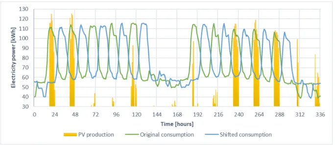
All the previous scenarios were based on original energy demand data, which represent typical energy user behaviour of company with five working days. The power demand pattern during two weeks in January can be seen in Fig. no. 7 with high demand through five days of the week during the day time. However, as it can be seen, the electricity demand peaks are overlapping with electricity price peaks. Therefore, the scenario 5 presents a case, when energy user behaviour is different. For this purpose, the power demand data were shifted by 12 hours as it can be seen in the figure.
10 20 30 40 50 60 70 80 90 0 48 96 144 192 240 288 336 384 432 480 528 576 624 672 720 768 816 864 912 960 Pr ice [€/MW h] Time [hours]
Figure 7, Original power demand (Castellum, 2018, see Appendix 1), shifted power demand & electricity price (Nord Pool, 2019)
4.7.6 Scenario 6, Energy storage capacity
The scenario 6 is investigating the effect of the energy storage capacity. For the case 6.1 the capacity of SE-HT-TES was decreased to 600 kWh. In the case 6.2 the thermal energy storage is reduced to 400 kWh. These two cases do not include paired case simulations when there is no energy storage as the change of the energy storage capacity does not have any effect on input values for the system without it.
5 RESULTS
As it was described in previous chapter, simulations of six scenarios were executed for system with and without energy storage system. In this chapter, the results from simulations are presented. All the simulations were executed with the same weather input data and the PV parameters were also kept constant for all the cases. Because of this, the PV electricity production was calculated to be always the same 279990 kWh per year.
5.1
Scenario 1, Basic scenario
Simulations in basic optimisation scenario were executed as it was described in part 4.6.1. The Table 3 contains technical data from the simulations of one year period. It can be seen from the number of cycles the battery cycle count is almost triple compared to SE-HT-TES. Electricity from grid presents the electricity that needs to be payed for. It can be seen that the heat demand from utility company for battery simulation remains the same as in the case,
when there is no energy storage installed in the system. In case the SE-HT-TES is
implemented, the total heat used from utility company was lowered by 1.3 MWh. It can also be seen from the column used electricity from PV and PV self-consumption that the energy storage systems increase these values, where originally, the PV self-consumption is 67 %. With SE-HT-TES the PV self-consumption reaches up to 98 % and only 2 % of the PV
electricity production is lost or fed back into the grid. Battery storage ensures 89 % of PV self-consumption. Self-sufficiency ratio represents the amount of electricity/energy demand satisfied from own PV source. It can be seen the battery installed in the system gives highest self-sufficient ratio for electricity. However, when it comes to self-sufficiency for both electricity and heat, the difference between battery storage and SE-HT-TES is 1 %. Although the total PV self-consumption in case 1.1B is lower, the self-sufficiency is higher than in case 1.1. This is caused by lower sum of energy which is taken from utility companies.
Table 3, Basic scenario, technical output
Number of cycles [-] Electricity from grid [kWh] Heat from utility [kWh] Used electricity from PV [kWh] PV self- consum-ption [-] Self-sufficiency ratio, electricity [-] Self-sufficiency ratio, tot. energy [-] 1.1 SE-HT-TES 40.2 389200 375080 275450 0.98 0.34 0.22 1.1N No ES - 403340 388560 186236 0.67 0.32 0.19 1.1B Battery 113.3 363380 388560 249510 0.89 0.38 0.23
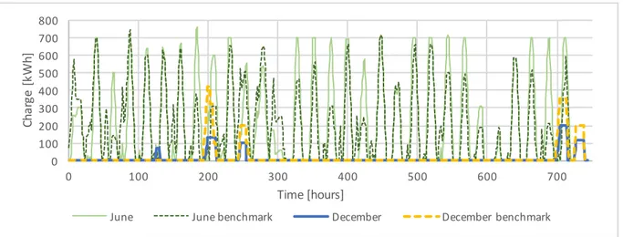
The Fig. 8 shows the SE-HT-TES state of charge through its one year operation. It can be seen, just as in the more detailed Fig. 9, the highest use of the energy storage is during the summer months. On the other hand, the use of SE-HT-TES is reduced during the winter period. The maximum energy stored in one moment it below 900 kWh when the total SE-HT-TES capacity is 2666 kWh. This means, that it was always less than 34 % of the maximum energy storage capacity which used during the one year simulation.
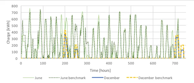
Below in the Figure 9 the SE-HT-TES state of charge during June and December is shown. It can be seen, that the energy storage is rarely used during the winter month. On the other hand, the SE-HT-TES is used regularly during June. Data from Figures 8 and 9 are used to be compared with results in other scenarios and it is referred as the “benchmark”.
Figure 9, SOC Thermal energy storage, month
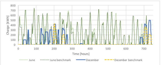
The Figure 10 shows the battery state of charge during case simulation 1.1B for the one year period. It can be seen that the battery energy storage is used more regularly compared to thermal energy storage. This can be seen especially during winter months in the beginning and at the end of the simulation period. It can also be seen, the total energy stored in the battery during the year never exceeds 700 kWh when the total battery capacity is 1111 kWh. This means maximally 63 % of the battery capacity is used.
Figure 10, SOC Battery storage, year
The Figure 11 shows the use of battery energy storage during June and December. Similarly, as in the case of SE-HT-TES, it can be seen the battery is used more often during summer month compared to December. However, it can also be seen that the battery is charged more often during winter compared to SE-HT-TES.
100 200 300 400 500 600 700 0 1000 2000 3000 4000 5000 6000 7000 8000 St at e of c ha rg e [k W h] Time [Hours]