2007 Central Plains irrigation conference, proceedings

(1)

CPIC Proceedings 2007

2007 Central Plains Irrigation Conference

Proceedings

COMPARISON OF SOIL WATER SENSING METHODS FOR

<!--[if

!supportNestedAnchors]-->

IRRIGATION MANAGEMENT AND RESEARCH

... 1

Steven R. Evett, Terry A. Howell, and Judy A. Tolk*

WATER SAVINGS FROM CROP RESIDUE MANAGEMENT No Online

Version

Norm Klocke, Randall Currie, Troy Dumler

CROP RESIDUE AND SOIL WATER

... 28

David Nielsen

CONVENTIONAL, STRIP AND NO TILLAGE CORN

PRODUCTION UNDER DIFFERENT IRRIGATION

CAPACITIES

... 32

Freddie Lamm and Rob Aiken Corrections to graphs on 4-3-07

STRATEGIES TO MAXIMIZE INCOME

WITH LIMITED WATER

... 48

Tom Trout

IRRIGATION WATER CONSERVING

STRATEGIES FOR CORN

... 53

Steve Melvin and Jose Payero

CRITERIA FOR SUCCESSFUL ADOPTION

OF SDI SYSTEMS

... 62

Danny Rogers and Freddie Lamm

SALT THRESHOLDS FOR LIQUID MANURE

APPLICATIONS THROUGH A CENTER PIVOT

... 72

Bill Kranz, Charles Shapiro, and Bill Wortmann

LAND APPLICATION OF ANIMAL WASTE

ON IRRIGATED FIELDS

... 79

Alan Schlegel, Loyd Stone, H. Dewayne Bond, and Mahbub Alam

(2)

CPIC Proceedings 2007

CENTER PIVOTS WHEN APPLYING WASTEWATER

... 88

Jake LaRue

INFLUENCE OF NOZZLE PLACEMENT ON

CORN GRAIN YIELD, SOIL MOISTURE AND RUNOFF

UNDER CENTER PIVOT IRRIGATION

... 93

Joel Schneekloth and Troy Bauder

ECONOMICS OF IRRIGATION ENDING DATE FOR CORN:

USING FIELD DEMONSTRATION RESULTS

... 99

Mahbub Alam, Troy Dumler, Danny Rogers, and Kent Shaw

CENTER PIVOT PRECISION MOBILE DRIP IRRIGATION

... 107

Brian Olson and Danny Rogers

USING YOUR RECORDS TO LOCATE INEFFICIENT

PUMPING PLANTS

... 114

Tom Dorn

COST OF PRODUCTION AND EQUITABLE LEASING

ARRANGEMENTS FOR CENTER PIVOT IRRIGATED

CORN IN CENTRAL NEBRASKA

... 118

(3)

COMPARISON OF SOIL WATER SENSING METHODS

FOR IRRIGATION MANAGEMENT AND RESEARCH

S.R. Evett*, T.A. Howell, and J.A. Tolk

Soil and Water Management Research Unit

USDA-ARS, Bushland, TX

*Voice: 806-356-5775, Fax: 806-356-5750

Email: srevett@cprl.ars.usda.gov

ABSTRACT

As irrigation water resources decrease and deficit irrigation becomes more

common across the Great Plains, greater accuracy in irrigation scheduling will be required. With deficit irrigation a smaller amount of soil water is held in reserve and there is less margin for error. Researchers investigating deficit irrigation practices and developing management practices must also have accurate measures of soil water content – in fact, the two go hand in hand. New management practices for deficit irrigation will require more accurate assessments of soil water content if success is to be ensured. This study

compared several commercial soil water sensing systems, four of them based on the electromagnetic (EM) properties of soil as influenced by soil water content, versus the venerable neutron moisture meter (NMM), which is based on the slowing of neutrons by soil water. While performance varied widely, the EM sensors were all less precise and less accurate in the field than was the NMM. Variation in water contents from one measurement location to the next was much greater for the EM sensors and was so large that these sensors are not useful for determining the amount of water to apply. The NMM is still the only sensor that is suitable for irrigation research. However, the NMM is not practical for on-farm irrigation management due to cost and regulatory issues. Unfortunately, our studies indicate that the EM sensors are not useful for irrigation management due to inaccuracy and variability. A new generation of EM sensors should be developed to overcome the problems of those currently available. In the

meantime, tensiometers, electrical resistance sensors and soil probes may fill the gap for irrigation management based on soil water sensing. However, many farmers are successfully using irrigation scheduling based on crop water use estimates from weather station networks and reference ET calculations. When used in conjunction with direct field soil water observations to avoid over irrigation, the ET network approach has proved useful in maximizing yields.

(4)

INTRODUCTION

For most uses and calculations in irrigation management and research, soil water content (θv, m3 m−3) is expressed as a volume fraction,

soil of volume total water soil of volume θ_v = [1]

Volume per volume units are used in most calculations of soil water movement and crop water uptake, including those in irrigation scheduling computer

programs or back-of-the-envelope checkbook type calculations. These units make it easy to convert water contents, θv, measured in a soil profile over a given depth, z, to an equivalent depth of water (θz) by multiplying the water content by the depth: θz = θv z. The units of θz are the length units of z, typically mm, cm or inches. For example, the depth of irrigation water, IzUL, that a uniform soil can accept without large losses to deep percolation is limited on the upper bound by the depth of the root zone, zr, and the difference between the mean water content of the root zone, θr, and the water content at field capacity, θFC; that is,

IzUL = zr(θFC – θr). For soils that have differences in soil texture with depth, similar calculations can be done layer by layer using the different texture-specific field capacity values and water contents available from most soil surveys or computer programs (e.g., http://staffweb.wilkes.edu/brian.oram/soilwatr.htm)..

Soil texture is quantified by the relative percentages by mass of sand, silt, and clay after removal of salts and organic matter. Both texture and structure determine the soil-water characteristic curve, which quantifies the relationship between soil water content and soil water potential, which is the strength with which the soil holds water against removal by plants. This relationship differs largely according to texture (Fig. 1), but can be strongly affected by organic matter and salt contents. The range of plant-available water (PAW) possible for a given soil is determined by two limits. The upper limit, also know as the field capacity, is often defined as the soil water content of a previously saturated soil after 24 h of free drainage into the underlying soil. The field capacity can be viewed as the water content below which the soil does not drain more rapidly than the crop can take up water. In heavier textured (i.e., more clayey) soils, this limit is often characterized as the water content at −0.10 kPa soil water potential. In more sandy (“lighter”) soils, the upper limit may be more appropriately placed at −0.33 kPa soil water potential. The difference in soil water potentials that are related to the upper limit of PAW is due to the relatively large conductivities for water flux in lighter soils near saturation, which means that lighter soils will drain more rapidly. The lower limit of PAW, also known as the permanent wilting point, is often defined as the soil water content at which the crop wilts and cannot recover if irrigated. The soil water potential associated with the lower limit varies with both the crop and the soil; but is often taken to be −1500 kPa. The amount of PAW differs greatly by soil texture. For example, as illustrated in Figure 1, a clay soil may have a plant available water content range of 0.19 to 0.33 m3 m−3,

(5)

or 0.14 m3_m−3_{PAW; whereas a silt loam may have a larger PAW content range} of 0.08 to 0.29 m3 m−3, or 0.21 m3 m−3 PAW. Sandy soils tend to have small amounts of PAW, such as the 0.04 m3 m−3 for the sandy loam illustrated in Fig. 1 or the 0.06 m3_m−3_{reported by Morgan et al. (2001a) for an agriculturally}

important fine sand in Florida. Thus, irrigation management often focuses on applying smaller amounts of water more frequently on sandy soils.

10 100 1000 10000 100000 1000000 0 0.1 0.2 0.3 0.4 0.5 Water content (m3 m-3) M at ric po te nt ia l ( -cm ) Silt loam Loamy Sand Clay Field capacity Wilting Pt.

Figure 1. The soil water content vs. soil water matric potential relationship for three soil

textures as predicted by the Rosetta pedotransfer model (Schaap et al., 2001).

Horizontal lines are plotted for the field capacity, taken as −333 cm (~−33 kPa), and for the wilting point, taken as −15 000 cm (~−1500 kPa).

Crops differ in their ability to extract water from the soil, with some crops not capable of extracting water to even −1500 kPa, and others able to extract more water, reaching potentials even more negative than -1500 kPa (Ratliff et al., 1983, Tolk, 2003) (Fig. 2). Confounding this issue is the soil type effect on rooting density and on the soil hydraulic conductivity, both of which influence the lower limit of PAW for a particular crop. The fact that soil properties vary with depth means that the lower limit of PAW may be best determined from field, rather than laboratory, measurements.

The available soil water holding capacity (AWHC) is a term used to describe the amount of water in the entire soil profile that is available to the crop. Because water in the soil below the depth of rooting is only slowly available, the AWHC is generally taken as the sum of water available in all horizons in the rooting zone, calculated for each horizon as the product of the horizon depth and the PAW for that horizon. For example, for a crop rooted in the A and B horizons of a soil the AWHC is the product of the PAW of the A horizon times its depth plus the PAW of the B horizon times the rooted depth in the B horizon (Table 1).

(6)

Figure 2. Deviation of the lower limit of water extraction, θLL, measured in the field using

a neutron probe, from that measured at −1500 kPa in the laboratory on soil cores taken at several depths in the soil. Data are for corn, sorghum and wheat crops grown in a Ulysses silt loam (Tolk, 2003).

Table 1. Example calculation of available water holding capacity (AWHC) in the rooting zone of a crop rooted to 0.95-m depth in a soil’s A and B horizons, each with a different value of plant available water (PAW).

Depth

range

Rooting depth

Rooted

depth PAW AWHC

Horizon (cm) (cm) (cm) (m3 m−3) (cm)

A, silt loam 0 to 20 0 to 20 20 × 0.21 = 4.2

B, clay 20 to 100 20 to 95 75 × 0.14 = 10.5

Sum 14.7

For irrigation scheduling using the management allowed depletion (MAD) concept (Fig. 3), irrigation is initiated when soil water has decreased to the θMAD level. The θMAD value may be chosen such that the soil never becomes dry enough to limit plant growth and yield, or it may be a smaller value that allows some plant stress to develop. Choice of the θMAD value needs to consider the irrigation capacity (flow rate per unit land area), which determines how quickly a given irrigation amount can be applied to a specified sized field. It is common to irrigate at some value of water content, θMAD+, that is larger than θMAD. This is done to ensure that the error in water content measurement, which may cause inadvertent over estimation of water content, is not likely to cause irrigation to be delayed until after water content is actually smaller than θMAD. Minimizing the difference, d = θMAD+ - θMAD, allows the irrigation interval to be increased. It is desirable to know the number of samples required to estimate the water content to within d of θMAD at the (1 – α) probability level. Knowing the sample standard deviation, S, of soil water content measurements, the required number of samples, n, can be estimated as

(7)

2 2 / _⎟ ⎠ ⎞ ⎜ ⎝ ⎛ = d S u n α [2]

where uα/2 is the (α/2) value of the standard normal distribution, and (1 – α) is the probability level desired (eg. 0.95 or 0.90). Equation [2] is valid for normally distributed values that are independent of one another and for the population standard deviation estimated from the sample standard deviation, S, of a large number of samples.

Figure 3. Illustration of the soil profile indicating fractions of the total soil volume (here

represented by unity) that are occupied by water at four key levels of soil water content. For this silty clay loam, the soil is full of water at saturation (0.42 m3_m−3_{), drains easily to}

field capacity (0.33 m3_m−3_{), and reaches the permanent wilting point (15 bars) at 0.18}

m3_m−3_{water content. To avoid stress in a crop such as corn, irrigations are scheduled}

when the soil water content reaches or is projected to reach 0.25 m3_m−3_{, the value of} θMAD for this soil and crop.

Because this analysis depends on the sample standard deviation determined by repeated readings with a particular device, it encapsulates the variability of readings from that device; but it does not include bias (non-random error) that may be present in the device readings due to, for example, inaccurate

calibration. Aside from large-scale spatial variability, the calibration is a potentially large source of error; and this error is not reduced by repeated sampling (Vauclin et al., 1984). Thus, careful field calibration is essential to minimize such bias (Hignett and Evett, 2002; Greacen, 1981). In most cases, this analysis may be applied to values of soil profile water storage that are calculated on the basis of samples at multiple depths.

(8)

For example using the data for the three soils in Fig. 1, the differences between the values of water content at field capacity, θFC, and at the permanent wilting point, θPWP, are the plant available water, θPAW (Table 2). Assuming that the management allowed depletion is 0.6 of θPAW, the allowable ranges of water content during irrigation scheduling are 0.126, 0.085, and 0.022 m3 m−3 for silt loam, clay, and loamy sand, respectively (Table 2). These narrow ranges place high accuracy demands on soil water sensing equipment. Assuming that soil-specific calibrations have been performed to minimize bias, and that the

accuracy of calibration is an acceptably small value (as determined by the RMSE of regression << MAD range), a specific sensor must still provide an acceptably precise mean value of field readings (that is, standard deviation of readings at multiple locations < MAD range).

Table 2. Example calculation of management allowed depletion (MAD, m3 m-3) in three soils with widely different textures. The small range of MAD severely tests the abilities of most soil water sensors, particularly for the loamy sand soil.

θFC θPWP θPAW MAD MAD

Horizon (m3 m−3) (m3 m−3) (m3 m−3) fraction (m3 m−3)

silt loam 0.086 0.295 0.209 × 0.6 = 0.126

loamy sand 0.066 0.103 0.037 × 0.6 = 0.022

clay 0.190 0.332 0.142 × 0.6 = 0.085

The ability to provide an acceptably precise mean value of field readings using a cost-effective number of access tubes or sensors in the soil is where some

sensors are lacking (Table 3). In particular, the capacitance sensors appear to be very sensitive to small-scale variations in soil water content, and thus require many more access tubes to attain a precision equal to that attained with much fewer NMM or gravimetric samples. Another example is data from Australia showing that the standard deviation of profile water contents reported by the EnviroSCAN system was 12.36 cm compared with S of 0.93 cm for the NMM in the same flood irrigation basin (Evett et al., 2002b).

If no other information were available about soil water variability, sampling a field for profile water content would typically require many profiles to be sampled, either directly or using water content sensor(s) in access tubes. However, distribution of profile water content tends to be temporally stable in some fields, at least over a growing season (Vachaud et al., 1985; Villagra et al., 1995). This means that there are locations in the field where the profile water content is usually very representative of the mean for the field, or of the extremes (Fig. 4) (Evett, 1989). Irrigators recognize this when they observe the crop in a field for water stress or when they probe the soil for water content. For example, an irrigator may ignore drier crops at the edge of a field, or a low, wet corner of the field when assessing the need to irrigate. The tendency is to make observations in places that show the mean behavior of the field. This is not an adequate way of choosing observation locations for a scientific experiment for which blocking,

(9)

randomization, replication and other considerations are required for statistical validity. But, for irrigation management in production agriculture, the choosing of measurement locations on the basis of observed soil and plant properties that are representative of the field may be the most cost effective and efficient method.

Table 3. Calculation using Eq. [2] of the number of access tubes (N) needed to find the mean profile water storage in a field to a precision d (cm) at the (1 - α) probability level (µα/2 is the value of the standard normal distribution at α/2) for a given field-measured standard deviation (S, cm) of profile storage. Data are from ten access tubes for each device, spaced at 10-m intervals in transects that were 5-m apart. α = 0.05 0.10 µα/2 = 1.96 1.64 d (cm) = 1 0.1 Method Soil condition S (cm) N N Diviner 2000† Irrigated 1.31 6.6 464 Dryland 2.42 22.5 1584 EnviroSCAN† Irrigated 1.52 8.9 625 Dryland 2.66 27.2 1914 Delta-T PR1/6† Irrigated 2.72 28.4 2002 Dryland 12.16 568.0 40006

Sentry 200AP†‡ Overall 3.78 54.9 3866

Trime T3 Irrigated 0.75 2.2 152

Dryland 2.38 21.8 1533

Gravimetric by Irrigated 0.45 0.8 55

push tube Dryland 0.70 1.9 133

CPN 503DR Irrigated 0.15 0.1 6

NMM Dryland 0.27 0.3 20

† Capacitance type sensors

‡ Estimated from data of Evett and Steiner (1995)

The previous paragraph not withstanding, the scheduling of irrigations on the basis of a single profile water content measurement in a field is prone to large errors. Also, there is strong evidence that actively growing vegetation can reduce or eliminate the temporal stability of water content, particularly in the root zone (Hupet and Vanclooster, 2002) and in fields with little topographic relief. A

reasonable minimum for the NMM or gravimetric sampling is three to four profile water content measurements at locations chosen to be representative of the field (Tollner et al., 1991). For other methods, such as the capacitance sensors, that sense smaller volumes resulting in larger values of S, the number of profile measurements needed may be much greater (Table 3).

(10)

A VER AGE R E LATIVE DIF F ER E NCE 1 0 -1 0 3 6 9 12 15 18 21 24 27 30 33 36 39 42 45 48 51 54 57 51 2 35 1434 3727 2425 11283 53 29 44 23 4534 30854 22 3821 327156 19 93649 57 52 18 335639 50 26 51431471340461716 551220 4148 10 42 RANK

Experiment 2, all irrigations, profile water content.

Figure 4. Ranking of locations by their average relative difference from the field mean

profile water content. Vertical bars indicate the range of values observed over the course of the experiment. Location 21 in particular was close to the mean profile water content at all times.

TWO FIELD STUDIES

Electromagnetic (EM) soil water sensing systems are rapidly entering the soil water sensor market. Common systems use sensors based on capacitance or time domain reflectometry (TDR) principles. For three capacitance soil water sensing systems (Sentek EnviroSCAN1, Sentek Diviner 2000, and Delta-T PR1/6), the Trime T3 quasi-TDR soil water sensing system, and the neutron moisture meter (NMM), we developed soil-specific calibrations for the A, Bt, and calcic Bt horizons of the Pullman soil at Bushland, TX (Evett et al., 2006). We applied these calibrations to data acquired in a wheat field in 2003 in order to investigate the variability of soil water estimates without the confounding factor of inaccurate factory calibrations. There were ten access tubes for each system, arranged in linear transects. After the first three measurement cycles, half of the winter wheat field (containing five access tubes) was irrigated to see how the five systems were able to sense the differences in water content. Access tubes were spaced 10-m apart. In addition to the five soil water sensing methods, gravimetric samples were taken with an hydraulic push probe (Giddings) in transects on some of the sampling dates. Sampling points were spaced 10-m apart; and samples were 10-cm in height and had a volume of 75.5 cm3. The data in Table 3 are from this study.

1_{The mention of trade or manufacturer names is made for information only and does not imply an}

(11)

Profile water contents reported by the six methods differed considerably (Figure 5), particularly in the degree of water content variability and the shape of the profile, which is influenced by over and under estimation of water content at different depths. The smallest variability of water content was reported by the NMM; and the NMM data matched the direct gravimetric data better than any other sensor. Variability of gravimetric measurements was only slightly larger than that of the NMM; and variability of Trime T3 results was somewhat more variable, but still representative of the profile water content in much the same way as the NMM. In this field, the depth to the CaCO3-enriched (caliche) layer was ~120 cm. As shown by the NMM and gravimetric results, inherent soil water variability was larger in the caliche horizon below 120 cm than in the Bt and A horizons above 120 cm. The larger variability below 120 cm is due to the

presence of prairie dog burrows that are present in the softer caliche soil (Fig. 5, right). These are invariably found in soil pits dug at the Bushland research station. The burrows contain soil that has washed in from the overlying Bt and A horizons; and they typically exhibit smaller bulk density than the overlying and surrounding soil. Depending on the presence or absence of macropore flow, typically occurring in soil cracks in the overlying A and Bt horizons of this soil, the soil in burrows may exhibit larger or smaller water content than surrounding soil. While all of the EM sensors exhibited more variability than the NMM, the three capacitance sensors exhibited the most variability as well as a tendency to severely underestimate water content in the A horizon above 50-cm depth. This could be indicative of a weakness in the soil-specific calibrations of Evett et al. (2006), or it might be due to poor contact of the plastic access tubes in this soil after more than seven months in the soil. Particularly near the top of the access tubes, vibration from repeated instrument insertion and extraction can cause small annular air spaces to develop between the soil and access tube. Also, shrinkage and swelling of the soil could create air space around the tubes near the surface where the soil is unconstrained. The NMM is not sensitive to such small air gaps, but they can permit water movement down the outside tube walls. The under estimation by the capacitance sensors was so consistent that we think it is due to a very strong dependency of the calibration equation coefficients on clay content of the soil, which increases strongly with depth in this soil. The variability in water contents illustrated in Fig. 5 is reflected in the values of S in Table 3.

A second study was done in a drip irrigated sweet pepper field near Five Points, CA, in the San Joaquin Valley on a Panoche clay loam soil in 2005. Data are presented for two periods in the season (Fig. 6). The first period was during the irrigation season as pepper fruits were developing; and the second period was during field dry down after irrigation had been suspended, but the crop was still transpiring. Sensors studied were the NMM, and three capacitance sensors: the Delta-T PR2/6 (successor to the PR1/6), the Sentek Diviner 2000 and the Sentek

(12)

EnviroSCAN. Data from the NMM showed that, below the surface, the soil water content profile was nearly uniform with depth at both dates, though the decrease in water content during dry down was evident. Gravimetric data (not shown) from the same field showed the same uniformity of water content with depth as did the NMM. Data from the PR2/6 indicated that the water content was much more variable, and that water content increased with depth during the dry down period. Neither indication is true. What is true is that this soil becomes increasingly saline during the irrigation season, and that salinity increases with depth in the profile at the end of the season. Thus, the increasing water contents with depth from the PR2/6 are the result of this sensor being sensitive to salinity, not an indication that water content increased with depth. Data shown are using the factory calibration for clay soils for the PR2/6, which resulted in both over and under estimation of water contents, depending on the depth. Data for the EnviroSCAN and Diviner 2000 for the same two periods are similar. They show more

variability than actually existed at the scale of crop water uptake; and similar to the PR2/6, they showed a false increase of water content with depth late in the season, probably due to salinity increasing with depth. Again, the use of factory calibrations resulted in some large over and under estimations of water content.

Figure 5. (Left) Profile water contents for ten transect locations for each of five sensor

systems, in a winter wheat field on 5 November, 2003, compared with gravimetric measurements. Half of the field (five transect locations) was irrigated. Sensing methods were frequency domain (EnviroSCAN, Diviner 2000, and PR1/6), quasi-TDR (Trime T3), and the neutron moisture meter (NMM). (Right) Photograph of the Pullman soil profile to 2-m depth showing the lighter colored caliche horizon.

(13)

A

B

Figure 6. Water content data from two periods for each sensor during a 2005 study in

California. The first period was during the irrigation season as pepper fruits were developing; and the second period was during field dry down after irrigation had been suspended, but the crop was still transpiring. Sensors studied were the NMM and the Delta-T PR2/6 (shown in A), and the Sentek Diviner 2000 and EnviroSCAN (B).

(14)

EFFECT OF SALINITY

World wide, 20% of irrigated soils are salt affected (Hachicha and Abd El-Gawed, 2003). Sensitivity to soil salinity, measured as the bulk electrical conductivity (BEC), limits the applicability of frequency domain or power loss sensors in many irrigated soils in which BEC varies across the field (Fig. 7) and with time (Fig 8). Variations of BEC of as much as 12 dS m−1 can occur over distances of less than one meter (Burt et al., 2003), and differences equally as large can occur from year to year or even within an irrigation season in one location (Hanson et al., 2003). Abdel gawad et al. (2003) measured periodic soil solution EC variations of 5 to 6 dS m−1 under drip irrigation in Syria. Mmolawa and Or (2000) measured a BEC change from 0.3 to 2.3 dS m−1_{in a few hours under drip irrigation of corn.} While it is possible to calibrate most sensors for a particular BEC, in these situations of temporally and spatially variable BEC, such a calibration is not applicable. From the available data, it is clear that errors larger than 50% in soil water content at a single location, and errors similarly large in soil profile water content are possible given the range of BEC values measured. Spatial and temporal variations of BEC are not confined to drip irrigation, but are present under furrow, flood, and sprinkler irrigation as well.

Figure 7. Variations in EC of saturation paste soil extracts (ECe) in two dimensions of a

(15)

Figure 8. Variations in EC from saturation paste soil extracts from a single location in a

drip-irrigated tomato field in California in two different years. No yield variation was found. (Hanson et al., 2003)

Sensors based on electromagnetic principles are often also sensitive to clay content and type even in non-saline soils. This is because clays exhibit varying degrees of charge and are associated with cations or anions in the soil solution to varying degrees. Commonly, clays exhibit negative charge and are associated with cations to a degree that is evaluated as the cation exchange capacity (CEC). As the soil content of high CEC clay increases, the soil becomes more

electrically lossy, that is, more capable of affecting the movement of electrical fields. This affects the frequency of oscillation of capacitance systems and the power loss of power loss systems in a way that is separate from, but not completely independent of, the soil water content. Examples include the much different calibration equations developed for the several soils existing under one center pivot irrigation system in France (Fig. 9) (Ruelle et al., 2003, personal communication), and the different calibration equations reported by Baumhardt et al. (2000) at Lubbock, TX, and Morgan et al. (1999) for the Sentek EnviroSCAN system.

(16)

Figure 9. Calibrations of the model CS615 soil water probe from Campbell Scientific,

Inc. in nine different soil layers of three different soils (A, B, and C), illustrating the wide variance in calibration equations for different layers in a particular soil and among soils (Ruelle et al., 2003, personal communication).

GRANULAR MATRIX SENSORS

Several types of granular matrix sensors (GMS) are on the market. The sensor consists of a porous medium in which are embedded two wires, often connected to wire mesh electrodes inside the sensor. The reading is of the electrical

resistance in the medium between the wires or mesh electrodes. Often, a quantity of gypsum (calcium sulfate) is included to buffer the soil water solution and decrease effects of salinity on the resistance. The greater the soil water tension, the less water is in the porous medium, and the greater the electrical resistance. Calibration may be done in a porous medium covering a pressure plate, which is subjected to several values of pressure in a pressure chamber. Calibrations are soil specific, so it is wise to use the soil to be measured as the porous medium. Installation and contact problems are similar to those for a tensiometer or gypsum block, including contact problems in coarse sands and shrink/swell clays. At tensions less than 30 kPa, Taber et al. (2002) found that tensiometers responded more rapidly than GMS sensors in silt loam, loam, and coarse sand. As with gypsum blocks, reading requires an alternating current to minimize effects of capacitive charge build up and ionization. Lack of precision and calibration drift over time may limit use of GMS for determining soil water potential gradients.

The useful range of readings is approximately −10 to −200 kPa matric potential, though Morgan et al. (2001b) were able to use GMS sensors to −5 kPa in a fine sand. Sensors may be manually read or data logged (resistance reading). Some

(17)

hysteresis is noted with these sensors; and they are temperature sensitive (as much as 20 kPa per 10°C, Shock, 2003). Like gypsum blocks, GMS may be installed to practically any useful depth, limited only by wire length. Fewer

problems with soil contact are noted with GMS. The usefulness of GMS systems for irrigation scheduling has been illustrated by work done with onions, potato (Fig. 10), alfalfa, and sugar beet in the Malheur Valley of Oregon (Shock, 2003; Shock et al., 2003). Because of soil and irrigation variability, at least six sensors should be used to provide data for irrigation scheduling (Shock, 2003). For irrigation science, the GMS can be useful if calibrated for the soil over a range of temperatures and soil water potentials, and if soil temperature is measured at the location of each sensor so that calibration corrections for temperature can be applied. Automatic irrigation scheduling has been successfully implemented using GMS for high-value row crops (Shock et al., 2002) and for landscapes (Qualls et al., 2001).

Figure 10. Soil water potential in a sprinkler-irrigated potato field as sensed with six

granular matrix sensors datalogged using a Hansen model AM400 data logger, showing very good control of soil water potential. Note the dry-down period at the end of the irrigation season (Shock et al., 2003)

DIRECT OBSERVATION

Direct observations can be very useful in guiding irrigation management. The soil feel and appearance method involves squeezing a ball of soil in the hand and comparing its feel and appearance to photographs that show the appearance of different soil textures at various water contents. The USDA-NRCS publishes a handy guide with the photographs and descriptions of how the soil feels in the

(18)

hand at different water contents. While it is an approximate guide, this method is fairly simple, and when used by an experienced irrigator can give the amount to irrigate. It does require a trip to field, during which the leaf and crop appearance can also be assessed (curl, color, wilting). Usually, these are apparent only after stress is enough to limit yield. The feel and appearance guide can be found at

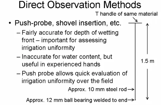
http://www.mt.nrcs.usda.gov/technical/ecs/agronomy/soilmoisture/index.html. Another method of direct observation common in irrigated Great Plains soils is the push probe (Fig. 11). The probe consists of a 3/8 or ½-inch diameter steel rod with a T handle at the top and a ball bearing of slightly larger diameter welded to the bottom end. The ball bearing makes a hole larger than the

diameter of the rod so that most of the resistance to penetration into the soil is at the ball, not due to friction between the soil and the rod. An experienced irrigator can fairly quickly assess variability in irrigation infiltration depth across a field, and perhaps most importantly can identify deep wetting of the profile that can result in deep percolation losses. Water lost to deep percolation carries with it costly fertilizers, the loss of which can reduce yield appreciably. Indeed, among farmers who have been over irrigating in the past, it is a common observation that reduction in water application is accompanied by increase in yield.

Figure 11. The push probe, a useful device for assessing irrigation penetration depth

(19)

CONCLUSIONS

The relatively expensive and high tech capacitance and other electromagnetic (EM) sensors are too inaccurate to be useful for assessing when and how much water to apply through irrigation. Sensitivities to soil bulk electrical conductivity, whether derived from clay type and content or from salt content, are too great with the current crop of EM sensors. A new generation of EM sensors should be developed to overcome the problems of those currently available. The neutron moisture meter, even though posing negligible health hazard, faces stiff

regulation and is useful mostly for research. Granular matrix sensors (resistance blocks) are useful in some soils and are particularly justified when produce quality is a concern. Direct observation remains the most used method of irrigation scheduling. Although not addressed in this paper, producers who can take advantage of a weather station network that provides crop water use estimates based on reference evapotranspiration are successfully using those networks to schedule irrigations. When used in conjunction with direct

observations (e.g. push probes) to avoid over irrigation, the ET network approach has proved useful in maximizing yields. One example is the Texas High Plains ET Network (http://txhighplainset.tamu.edu/) (Howell, 1998; Howell et al., 1998; Marek et al., 1998). For a more in-depth and technical discussion of soil water properties and soil water sensing systems, see Evett (2007).

REFERENCES

Abdel gawad, G., A. Arslan, A. Gaihbe, and F. Kadouri. 2003. The effects of saline irrigation water management and salt tolerant tomato varieties on sustainable production of tomato in Syria (1999-2002). Sustainable Strategies for Irrigation in Salt-prone

Mediterranean Region: A System Approach. Proc. International Workshop. Cairo, Egypt, Dec. 8-10, 2003. Centre for Ecology and Hydrology, Wallingford, UK. Dec. 2003.

Baumhardt, R.L., R.J. Lascano, and S.R. Evett. 2000. Soil material, temperature, and salinity effects on calibration of multisensor capacitance probes. Soil Sci. Soc. Amer. J. Vol. 64, No. 6. pp. 1940-1946.

Burt, C.M., B. Isbell, and L. Burt. 2003. Long-term salinity buildup on Drip/Micro irrigated trees in California. In "Understanding & Addressing Conservation and Recycled Water Irrigation", Proceedings of the International Irrigation Association Technical Conference. Pp. 46-56. November 2003. (CD-ROM)

Evett, S.R. 1989. Field investigations of evaporation from a bare soil. Ph.D. dissertation, Dept. of Soil and Water Science, College of Agriculture, University of Arizona, Tucson, AZ 85721. Available at

http://www.cprl.ars.usda.gov/wmru/srevett/dissertation.html.

Evett, S.R. Soil Water and Monitoring Technology. 2007. Chapter 2. Irrigation of Agricultural Crops. American Society of Agronomy, Crop Science Society of America, Soil Science Society of America, Madison, WI. In press.

Evett, S.R., and J.L. Steiner. 1995. Precision of neutron scattering and capacitance type moisture gages based on field calibration. Soil Sci. Soc. Amer. J. 1995. 59:961-968. Evett, Steven, Jean-Paul Laurent, Peter Cepuder, and Clifford Hignett. 2002b.

(20)

Compared on Four Continents. 17th World Congress of Soil Science, August 14-21, 2002, Bangkok, Thailand, Transactions, pp. 1021-1 - 1021-10. (CD-ROM).

Evett, S.R., J.A. Tolk, and T.A. Howell. 2006. Soil profile water content determination: Sensor accuracy, axial response, calibration, temperature dependence and precision. Vadose Zone J. 5:894–907.

Greacen, E.L. (ed.) 1981. Soil Water Assessment by the Neutron Method, CSIRO, Melbourne, Australia.

Hachicha, M., and G. Abd El-Gawed. 2003. Aspects of salt-affected soils in the Arab world. In Sustainable Strategies for Irrigation in Salt-prone Mediterranean Region: A System Approach. Proc. International Workshop, Cairo, Egypt, Dec. 8-10, 2003. Centre for Ecology and Hydrology, Wallingford, UK. ISBN 1 903741 08 4. pp. 295-310.

Hanson, B., D. May, and W. Bendixen. 2003. Drip irrigation in salt affected soil. In "Understanding & Addressing Conservation and Recycled Water Irrigation", Proceedings of the International Irrigation Association Technical Conference. Pp. 57-65. November 2003. (CD-ROM).

Hignett, C., and S.R. Evett. 2002. Neutron Thermalization. Section 3.1.3.10 In Jacob H. Dane and G. Clarke Topp (eds.) Methods of Soil Analysis. Part 4 – Physical Methods. pp. 501-521.

Howell, T. A. 1998. Using the PET network to improve irrigation water management. In Proc. The Great Plains Symposium 1998: The Ogallala Aquifer, March 10-12, 1998. pp. 38-45.

Howell, Terry, Marek, Thomas, New, Leon, and Dusek, Don. 1998. Weather network defends Texas water tables. Irrig.Business & Technology VI(6):16-20.

Marek, Thomas H., New, L. Leon, Howell, Terry A., Dusek, Don, Fipps, Guy, and Sweeten, John. 1998. Potential evapotranspiration networks in Texas: Design, coverage and operation. In Proc. 25th Water Conf. for Texas. Water Planning Strategies for Senate Bill 1, Texas Water Resources Institute and Texas A&M University System. pp. 115-124.

Hupet, F., and M. Vanclooster. 2002. Intraseasonal dynamics of soil moisture variability within a small agricultural maize cropped field. J. Hydrology. Vol. 261. pp. 86-101.

Morgan, K.T., L.R. Parsons, T.A. Wheaton, D.J. Pitts, and T.A. Obreza. 1999. Field calibration of a capacitance water content probe in fine sand soils. Soil Sci. Soc. Am. J. Vol. 63. pp. 987-989.

Morgan, K.T., T.A. Obreza, T.A. Wheaton, and L.R. Parsons. 2001a. Comparison of soil matric potential measurements using tenisometric and resistance methods. Proc. Soil Crop Sci. Soc. Florida. Vol. 61, June 10-12, pp. 63-66.

Morgan, K.T., L.R. Parsons, and T.A. Wheaton. 2001b. Comparison of laboratory- and field-derived soil water retention curves for a find sand using tensiometric, resistance and capacitance methods. Plant and Soil. Vol. 234. pp. 153-157.

Qualls, R.J., J.M. Scott, and W.B. DeOreo. 2001. Soil moisture sensors for urban landscape irrigation: effectiveness and reliability. J. Am. Water Resour. Assoc. June 2001. v. 37 (3) p. 547-559.

Ratliff, L.F., J.T. Ritchie, and D.K. Cassel. 1983. Field-measured limits of soil water availability as related to laboratory-measured properties. Soil Sci. Soc. Am. J. Vol. 47, pp. 770-775.

Schaap, M.G., F.J. Leij, and T. van Genuchten. 2001. ROSETTA: a computer program for estimating soil hydraulic parameters with hierarchical pedotransfer functions. J. Hydrol. Oct 1, 2001. v. 251 (3/4) p. 163-176.

(21)

Shock, C.C. 2003. Soil water potential measurement by granular matrix sensors. Pp. 899-903 In B.A. Stewart and Terry A. Howell (eds.). Encyclopedia of Water Science, Marcel Dekker, Inc. New York, NY.

Shock, C.C., E.B.G. Feibert, L.D. Saunders. 2002. Plant population and nitrogen fertilization for subsurface drip-irrigated onions. pp. 71-80 In Special Report 1038.

(http://www.cropinfo.net/AnnualReports/2001/ondrip01.htm; accessed 31 March 2004).

Also see: (http://www.cropinfo.net/granular.htm) Oregon State University Agricultural Experiment Station.

Shock, C.C., K. Kimberling, A. Tschida, K. Nelson, L. Jensen, and C.A. Shock, 2003. Soil moisture based irrigation scheduling to improve crops and the environment. pp. 227-234 In Special Report 1048.

(http://www.cropinfo.net/AnnualReports/2002/Hansen2002.htm) Oregon State University

Agricultural Experiment Station.

Taber, H.G., V. Lawson, B. Smith, and D. Shogren. 2002. Scheduling microirrigation with tensiometers or Watermarks. International Water Irrig. Vol. 22, No. 1. pp. 22-23, 26. Tolk, J.A. 2003. Plant Available Soil Water. Pp. 669-672 In B.A. Stewart and Terry A. Howell (eds.). Encyclopedia of Water Science. Marcel Dekker, Inc., New York, NY. Tollner, E.W., A.W. Tyson, and R.B. Beverly. 1991. Estimating the number of soil-water measurement stations required for irrigation decisions. Appl. Engr. Agric. Vol. 7, No. 2, pp. 198-204.

Vachaud, G., A. Passerat De Silans, P. Balabanis, and M. Vauclin. 1985. Temporal stability of spatially measured soil water probability density function. Soil Sci. Soc. Am. J. 49:822-828.

Vauclin, M., R. Haverkamp, and G. Vachaud. 1984. Error analysis in estimating soil water content from neutron probe measurements: 2. Spatial standpoint. Soil Sci. Vol. 137, No. 3, pp. 141-148.

Villagra, M.M., O.O.S. Bacchi, R.L. Tuon, and K. Reichardt. 1995. Difficulties of estimating evapotranspiration from the water balance equation. Agric. Forest Meteor. Vol. 72. pp. 317-325.

(22)

CROP RESIDUE AND SOIL WATER

D.C. Nielsen

Research Agronomist

USDA-ARS

Central Great Plains Research Station

Akron, CO

Voice: 970-345-0507 Fax: 970-345-2088

Email:

David.Nielsen@ars.usda.gov

INTRODUCTION

Final crop yield is greatly influenced by the amount of water that moves from the soil, through the plant, and out into the atmosphere (transpiration). Generally, the more water that is in the soil and available for transpiration, the greater the yield. For example, dryland wheat yield is strongly tied to the amount of soil water available at wheat planting time (Fig. 1). In this case an additional inch of water stored in the soil at wheat planting time would increase yield by 5.3 bu/a. For wheat selling at $4.00/bu, that inch of stored soil water is worth over $21/a. Similar relationships can be defined for other crops. But the point is that in the Great Plains where precipitation is low and erratic, an important production factor is storing as much of the precipitation and irrigation that hits the soil surface as possible.

Fig. 1. Relationship between winter wheat grain yield and available soil water at wheat planting at Akron, CO.

FACTORS AFFECTING WATER STORAGE

Time of Year/Soil Water Content

The amount of precipitation that finally is stored in the soil is determined by the precipitation storage efficiency (PSE). PSE can vary with time of year and the

Available Soil Water (in)

0 2 4 6 8 10

Wheat Yield (bu/a

) 0 10 20 30 40 50 60 70 1993 1995 1996 1997 1999 2001 bu/a = 5.56 + 5.34*in r2 = 0.76

(23)

water content of the soil surface. During the summer months air temperature is very warm, with evaporation of precipitation occurring quickly before the water can move below the soil surface. Farahani et al. (1998) showed that precipitation storage efficiency during the 2 ½ months (July 1 to Sept 15) following wheat harvest averaged 9%, and increased to 66% over the fall, winter, and spring period (Sept 16 to April 30) (Fig. 2). The higher PSE during the fall, winter, and spring is due to cooler temperatures, shorter days, and snow catch by crop residue. From May 1 to Sept 15, the second summerfallow period, precipitation storage efficiency averaged -13% as water that had been previously stored was actually lost from the soil. The soil surface is wetter during the second

summerfallow period, slowing infiltration rate, and increasing the potential for water loss by evaporation.

Fig. 2. Precipitation Storage Efficiency (PSE) variability with time of year. (after Farahani, 1998)

Residue Mass and Orientation

Studies conducted in Sidney, MT, Akron, CO, and North Platte, NE (Fig. 3) demonstrated the effect of increasing amount of wheat residue on the

precipitation storage efficiency over the 14-month fallow period between wheat crops.

Fig. 3. Precipitation Storage Efficiency (PSE) as influenced by wheat residue on the soil surface. (after Greb et al., 1967)

As wheat residue on the soil surface increased from 0 to 9000 lb/a, precipitation storage efficiency increased from 15% to 35%. Crop residues reduce soil water evaporation by shading the soil surface and reducing convective exchange of water vapor at the soil-atmosphere interface. Additionally, reducing tillage and

PSE ( % ) -20 0 20 40 60 80 July 1- Sept 15 Sept 16-April 30 May 1-Sept 15 Residue Level (lb a-1) 0 2000 4000 6000 8000 10000

PSE (%)

0

10

20

30

Sidney, MT Akron, CO North Platte, NE

(24)

maintaining surface residues reduce precipitation runoff, increase infiltration, and minimize the number of times moist soil is brought to the surface, thereby

increasing precipitation storage efficiency (Fig. 4).

Fig. 4. Precipitation Storage Efficiency (PSE) as influenced by tillage method in the 14-month fallow period in a winter wheat-fallow production system. (after Smika and Wicks, 1968; Tanaka and Aase, 1987)

Snowfall is an important fraction of the total precipitation falling in the central Great Plains, and residue needs to be managed in order to harvest this valuable resource. Snowfall amounts range from about 16 inches per season in southwest Kansas to 42 inches per season in the Nebraska panhandle. Akron, CO

averages 12 snow events per season, with three of those being blizzards. Those 12 snow storms deposit 32 inches of snow with an average water content of 12%, amounting to 3.8 inches of water. Snowfall in this area is extremely efficient at recharging the soil water profile due in large part to the fact that 73% of the water received as snow falls during non-frozen soil conditions.

Standing crop residues increase snow deposition during the overwinter period. Reduction in wind speed within the standing crop residue allows snow to drop out of the moving air stream. The greater silhouette area index (SAI) through which the wind must pass, the greater the snow deposition (SAI =

height*diameter*number of stalks per unit ground area). Data from sunflower plots at Akron, CO showed a linear increase in soil water from snow as SAI increased in years with average or above average snowfall and number of blizzards. Typical values of SAI for sunflower stalks (0.03 to 0.05) result in an overwinter soil water increase of about 4 to 5 inches (Fig. 5).

Fig. 5. Influence of sunflower silhouette area index on over-winter soil water change at Akron, CO. (after Nielsen, 1998) Tillage Method

PSE (%)

0

10

20

30

40

50

_{North Platte, NE} Sidney, MT Plow Stubble Mulch Red. Till No Till 0.00 0.02 0.04 0.06 0.08 Soi l Water Ch an ge (in )

0

2

4

6

8

10

(25)

Because crop residues differ in orientation and amount, causing differences in evaporation suppression and snow catch, we see differences in the amount of soil water recharge that occurs (Fig. 6). The 5-year average soil water recharge occurring over the fall, winter, and spring period in a crop rotation experiment at Akron, CO shows 4.6 inches of recharge in no-till wheat residue, and only 2.5 inches of recharge in conventionally tilled wheat residue. Corn residue is nearly as effective as no-till wheat residue in recharging soil water, while millet residue gives results similar to conventionally tilled wheat residue.

Fig. 6. Change in soil water content due to crop residue type at Akron, CO.

Good residue management through no-till or reduced-till systems will result in increased soil water availability at planting. This additional available water will increase yield in both dryland and limited irrigation systems by reducing level of water stress a plant experiences as it enters the critical reproductive growth stage.

REFERENCES

Farahani, H.J., G.A. Peterson, D.G. Westfall, L.A. Sherrod, and L.R. Ahuja. 1998. Soil water storage in dryland cropping systems: The significance of cropping intensification. Soil Sci. Soc. Am. J. 62:984-991.

Greb, B.W, D.E. Smika, and A.L. Black. 1967. Effect of straw mulch rates on soil water storage during summer fallow in the Great Plains. Soil Sci. Soc. Am. Proc. 31:556-559.

Nielsen, D.C. 1998. Snow catch and soil water recharge in standing sunflower residue. J. Prod. Agric. 11:476-480.

Smika, D.E., and G.A. Wicks. 1968. Soil water storage during fallow in the central Great Plains as influenced by tillage and herbicide treatments. Soil Sci. Soc. Am. Proc. 32:591-595.

Tanaka, D.L., and J.K. Aase. 1987. Fallow method influences on soil water and precipitation storage efficiency. Soil Till. Res. 9:307-316.

Residue Type

Wheat(CT) Wheat(NT) Corn Millet

Cha nge in Soi l Water (in ) 0 1 2 3 4 5 October-April (2000-2004)

(26)

CONVENTIONAL, STRIP, AND NO TILLAGE CORN

PRODUCTION UNDER DIFFERENT IRRIGATION

CAPACITIES

Dr. Freddie Lamm

Research Irrigation Engineer

Email:

flamm@ksu.edu

Dr. Rob Aiken

Research Crop Scientist

Email:

raiken@ksu.edu

KSU Northwest Research-Extension Center

105 Experiment Farm Road, Colby, Kansas

Voice: 785-462-6281 Fax: 785-462-2315

ABSTRACT

Corn production was compared from 2004 to 2006 for three plant populations (25,400, 28,600 or 32,000 plants /acre) under conventional, strip and no tillage systems for irrigation capacities limited to 1 inch every 4, 6 or 8 days. Corn yield increased approximately 12% from the lowest to highest irrigation capacity in these three years of varying precipitation and near normal crop

evapotranspiration. Strip tillage and no tillage had 8.8% and 7% higher grain yields than conventional tillage, respectively. Results suggest that strip tillage obtains the residue benefits of no tillage in reducing evaporation losses without the yield penalty sometimes occurring with high residue. The small increases in total seasonal water use (< 1.5 inch) for strip tillage and no-tillage compared to conventional tillage can probably be explained by the higher grain yields for these tillage systems.

INTRODUCTION

Declining water supplies and reduced well capacities are forcing irrigators to look for ways to conserve and get the best utilization from their water. Residue

management techniques such as no tillage or conservation tillage have been proven to be very effective tools for dryland water conservation in the Great Plains. However, adoption of these techniques is lagging for continuous irrigated corn. There are many reasons given for this lack of adoption, but some of the major reasons expressed are difficulty handling the increased level of residue from irrigated production, cooler and wetter seedbeds in the early spring which may lead to poor or slower development of the crop, and ultimately a corn grain yield penalty as compared to conventional tillage systems. Under very high production systems, even a reduction of a few percentage points in corn yield can have a significant economic impact. Strip tillage might be a good

compromise between conventional tillage and no tillage, possibly achieving most of the benefits in water conservation and soil quality management of no tillage, while providing a method of handling the increased residue and increased early growth similar to conventional tillage. Strip tillage can retain surface residues

(27)

and thus suppress soil evaporation and also provide subsurface tillage to help alleviate effects of restrictive soil layers on root growth and function. A study was initiated in 2004 to examine the effect of three tillage systems for corn production under three different irrigation capacities. Plant population was an additional factor examined because corn grain yield increases in recent years have been closely related to increased plant populations.

GENERAL STUDY PROCEDURES

The study was conducted under a center pivot sprinkler at the KSU Northwest Research-Extension Center at Colby, Kansas during the years 2004 to 2006. Corn was also grown on the field site in 2003 to establish residue levels for the three tillage treatments. The deep Keith silt loam soil can supply about 17.5 inches of available soil water for an 8-foot soil profile. The climate can be

described as semi-arid with a summer precipitation pattern with an annual rainfall of approximately 19 inches. Average precipitation is approximately 12 inches during the 120-day corn growing season.

A corn hybrid of approximately 110 day relative maturity (Dekalb DCK60-19 in 2004 and DCK60-18 in 2005 and 2006) was planted in circular rows on May 8, 2004, April 27, 2005 and April 20, 2006, respectively. Three seeding rates (26,000, 30,000 and 34,000 seeds/acre) were superimposed onto each tillage treatment in a complete randomized block design.

Irrigation was scheduled with a weather-based water budget, but was limited to the 3 treatment capacities of 1 inch every 4, 6, or 8 days. This translates into typical seasonal irrigation amounts of 16-20, 12-15, 8-10 inches, respectively. Each of the irrigation capacities (whole plot) were replicated three times in pie-shaped sectors (25 degree) of the center pivot sprinkler (Figure 1). Plot length varied from to 90 to 175 ft, depending on the radius of the subplot from the center pivot point. Irrigation application rates (i.e. inches/hour) at the outside edge of this research center pivot were similar to application rates near the end of full size systems. A small amount of preseason irrigation was conducted to bring the soil water profile (8 ft) to approximately 50% of field capacity in the fall and as necessary in the spring to bring the soil water profile to approximately 75% in the top 3 ft prior to planting. It should be recognized that preseason irrigation is not a recommended practice for fully irrigated corn production, but did allow the three irrigation capacities to start the season with somewhat similar amounts of water in the profile.

The three tillage treatments (Conventional tillage, Strip Tillage and No Tillage) were replicated in a Latin-Square type arrangement in 60 ft widths at three different radii (Centered at 240, 300 and 360 ft.) from the center pivot point (Figure 1). The various operations and their time period for the three tillage treatments are summarized in Table 1. Planting was in the same row location each year for the Conventional Tillage treatment to the extent that good farming

(28)

practices allowed. The Strip Tillage and No-Tillage treatments were planted between corn rows from the previous year.

Figure 1. Physical arrangement of the irrigation capacity and tillage treatments.

Fertilizer N for all 3 treatments was applied at a rate of 200 lb/acre in split applications with approximately 85 lb/ac applied in the fall or spring application, approximately 30 lb/acre in the starter application at planting and approximately 85 lb/acre in a fertigation event near corn lay-by. Phosphorus was applied with the starter fertilizer at planting at the rate of 45 lb/acre P2O5. Urea-Ammonium-Nitrate (UAN 32-0-0) and Ammonium Superphosphate (10-34-0) were utilized as the fertilizer sources in the study. Fertilizer was incorporated in the fall

concurrently with the Conventional Tillage operation and applied with a mole knife during the Strip Tillage treatment. Conversely, N application was broadcast with the No Tillage treatment prior to planting.

A post-plant, pre-emergent herbicide program of Bicep II Magnum and Roundup Ultra was applied. Roundup was also applied post-emergence prior to lay-by for all treatments, but was particularly beneficial for the strip and no tillage

treatments. Insecticides were applied as required during the growing season.

Weekly to bi-weekly soil water measurements were made in 1-ft increments to 8- ft. depth with a neutron probe. All measured data was taken near the center of each plot. These data were utilized to examine treatment differences in soil water conditions both spatially (e.g. vertical differences) and temporally (e.g.

(29)

differences caused by timing of irrigation in relation to evaporative conditions as affected by residue and crop growth stage).

(30)

Table 1. Tillage treatments, herbicide and nutrient application by period.

Period Conventional tillage Strip Tillage No Tillage

Fall 2003

1) One-pass chisel/disk plow at 8-10 inches with

broadcast N, November 13, 2003.

1) Strip Till + Fertilizer (N) at 8-10 inch depth,

November 13, 2003. 2) Plant + Banded starter N &

P, May 8, 2004.

2) Plant + Banded starter N & P, May 8, 2004

1) Broadcast N + Plant + Banded starter N & P, May 8, 2004 Spring 2004 _{3) Pre-emergent herbicide} application, May 9, 2004. 3) Pre-emergent herbicide application, May 9, 2004. 2) Pre-emergent herbicide application, May 9, 2004. 4) Roundup herbicide

application near lay-by, June 9, 2004

4) Roundup herbicide application near lay-by, June 9, 2004

3) Roundup herbicide application near lay-by, June 9, 2004 Summer 2004 5) Fertigate (N), June 10, 2004 5) Fertigate (N), June10, 2004 4) Fertigate (N), June 10, 2004 Fall 2004

1) One-pass chisel/disk plow

at 8-10 inches with

broadcast N, November 05, 2004.

Too wet, no tillage operations

1) Strip Till + Fertilizer (N) at 8-10 inch depth, March 15, 2005.

2) Plant + Banded starter N & P, April 27, 2005.

2) Plant + Banded starter N & P, April 27, 2005

1) Broadcast N + Plant + Banded starter N & P, April 27, 2005 Spring 2005 3) Pre-emergent herbicide application, May 8, 2005. 3) Pre-emergent herbicide application, May 8, 2005. 2) Pre-emergent herbicide application, May 8, 2005. 4) Roundup herbicide

3) Roundup herbicide application near lay-by, June 9, 2005 Summer 2005 5) Fertigate (N), June 17, 2005 5) Fertigate (N), June 17, 2005 4) Fertigate (N), June 17, 2005 Fall 2005

1) One-pass chisel/disk plow at 8-10 inches with

broadcast N, November 10, 2005.

1) Strip Till + Fertilizer (N) at 8-10 inch depth,

November 10, 2005. 2) Plant + Banded starter N &

P, April 20, 2006.

2) Plant + Banded starter N & P, April 20, 2006

1) Broadcast N + Plant + Banded starter N & P, April 20, 2006 Spring 2006 _{3) Pre-emergent herbicide} application, April 22, 2006. 3) Pre-emergent herbicide application, April 22, 2006. 2) Pre-emergent herbicide application, April 22, 2006. 4) Roundup herbicide

3) Roundup herbicide application near lay-by, June6, 2006 Summer 2006 5) Fertigate (N), June 13, 2006 5) Fertigate (N), June 13, 2006 4) Fertigate (N), June 13, 2006

(31)

140 160 180 200 220 240 260

Day of year

0 4 8 12 16 20 24

E

T

c

o

r P

re

c

ip

it

a

tio

n

(

in

c

h

e

s

)

_{ETc, 2004} ETc, 2005 ETc, 2006 ETc, Avg. 1972-2006 Rain, 2004 Rain, 2005 Rain, 2006 Rain, Avg. 1972-2006

Similarly, corn yield was measured in each of the 81 subplots at the end of the season. In addition, yield components (above ground biomass, plants/acre ears/plant, kernels/ear and kernel weight) were determined to help explain the treatment differences. Water use and water use efficiency were calculated for each subplot using the soil water data, precipitation, applied irrigation and crop yield.

RESULTS AND DISCUSSION

Weather Conditions

Summer seasonal precipitation was approximately 2 inches below normal in 2004, near normal in 2005, and nearly 3 inches below normal in 2006 at 9.99, 11.95 inches, and 8.99 inches, respectively for the 120 day period from May 15 through September 11 (long term average, 11.86 inches). In 2004, the last month of the season was very dry but the remainder of the season had

reasonably timely rainfall and about normal crop evapotranspiration (Figure 2). In 2005, precipitation was above normal until about the middle of July and then there was a period with very little precipitation until the middle of August. This dry period in 2005 also coincided with a week of higher temperatures and high crop evapotranspiration near the reproductive period of the corn (July 17-25). In 2006, precipitation lagged behind the long term average for the entire season. Fortunately, seasonal evapotranspiration was near normal as it also was for the other two years (long term average of 23.07 inches).

Figure 2. Corn evapotranspiration and summer seasonal rainfall for the 120 day period, May 15 through September 11, KSU Northwest Research-Extension Center, Colby Kansas.

(32)

140 160 180 200 220 240 260 Day of year 0 4 8 12 16 Ir ri ga ti on a m ount ( inc he s ) Limited to 1 in/4 d Limited to 1 in/6 d Limited to 1 in/8 d 2004 140 160 180 200 220 240 260 Day of year 0 4 8 12 16 Ir ri ga ti on a m ount ( inc he s ) Limited to 1 in/4 d Limited to 1 in/6 d Limited to 1 in/8 d 2005

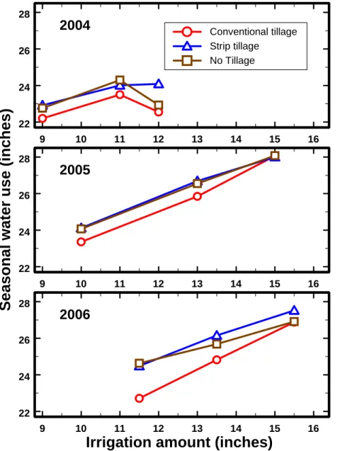
Irrigation requirements were lowest in 2004 with the 1 inch/4 day treatment receiving 12 inches, the 1 inch/ 6 day treatment receiving 11 inches and the 1 inch/8 day treatment receiving 9 inches (Figure 3).

Figure 3. Seasonal irrigation for the 120 day period, May 15 through September 11, 2004 for the three irrigation treatments in an irrigation capacity and tillage study, KSU Northwest Research-Extension Center, Colby Kansas.

The irrigation amounts in 2005 were 15, 13, and 10 inches for the three respective treatments (Figure 4).

(33)

140 160 180 200 220 240 260 Day of year 0 4 8 12 16 Ir ri ga ti on a m ount ( inc he s ) Limited to 1 in/4 d Limited to 1 in/6 d Limited to 1 in/8 d 2006

The irrigation amounts were highest in 2006 at 15.5, 13.5, and 11.50 inches for the three respective treatments (Figure 5).

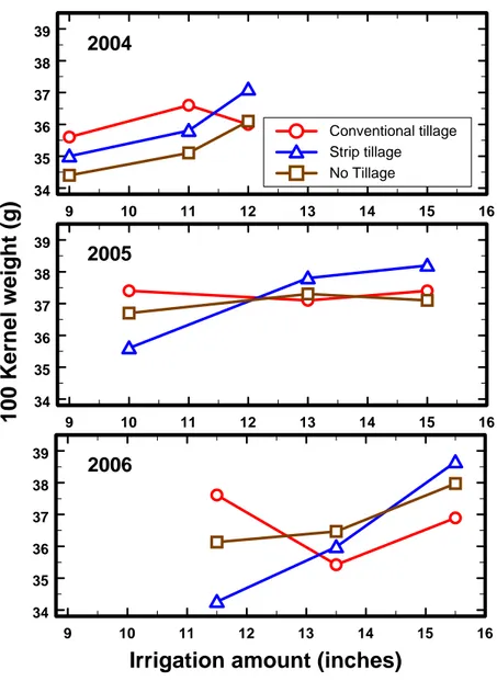
Crop Yield and Selected Yield Components

Corn yield was relatively high for all three years ranging from 161 to 262 bu/acre Table 2 through 4, and Figure 6). Higher irrigation capacity generally increased grain yield, particularly in 2005 and 2006. Strip tillage and no tillage had higher grain yields at the lowest irrigation capacity in 2004 and at all irrigation capacities in 2005 and 2006. Strip tillage tended to have the highest grain yields for all tillage systems and the effect of tillage treatment was greatest at the lowest irrigation capacity. These results suggest that strip tillage obtains the residue benefits of no tillage in reducing evaporation losses without the yield penalty sometimes associated with the higher residue levels in irrigated no tillage management.

Higher plant population had a significant effect in increasing corn grain yields (Tables 2 through 4, Figure 7) on the average about 10 to 20 bu/a for the lowest and highest irrigation capacities, respectively. Higher plant population gives greater profitability in good production years. Assuming a seed cost of

$1.49/1,000 seeds and corn harvest price of $3.75/bushel, this 14 to 20 bu/acre yield advantage would increase net returns approximately $27 to $65/acre for the increase in plant population of approximately 6,100 seeds/acre. Increasing the plant population by 6100 plants/a on the average reduced kernels/ear by 48 and reduced kernel weight by 1.5 g/100 kernels (Tables 2 through 4). However, this

(34)

was compensated by the increase in population increasing the overall number of kernels/acre by 12.8% (data not shown).

Table 2. Selected corn yield component and total seasonal water use data for 2004 from an irrigation capacity and tillage study, KSU Northwest Research-Extension Center, Colby, Kansas.

Irrigation Capacity Tillage System Target Plant Population (1000 p/a) Grain Yield bu/acre Plant Population (p/a) Kernels /Ear Kernel Weight g/100 Water Use (inches)

1 in/4 days Conventional 26 229 27878 550 37.1 23.0

(12 inches) 30 235 29330 557 36.2 22.6 34 234 32234 529 34.6 22.0 Strip Tillage 26 245 27588 537 38.9 23.5 30 232 30492 519 37.0 24.4 34 237 33106 514 35.5 24.3 No Tillage 26 218 25846 548 37.7 22.0 30 226 29330 539 36.8 23.6 34 251 33686 553 33.8 23.2

(35)

Table 3. Selected corn yield component and total seasonal water use data for 2005 from an irrigation capacity and tillage study, KSU Northwest Research-Extension Center, Colby, Kansas.

Irrigation Capacity Tillage System Target Plant Population (1000 p/a) Grain Yield bu/acre Plant Population (p/a) Kernels /Ear Kernel Weight g/100 Water Use (inches)

2007 Central Plains irrigation conference, proceedings