Evaluation of Roadway Embankment Under Repetitive Axial Loading Using Finite Element Analysis

(1)

Evaluation of Roadway Embankment

Under Repetitive Axial Loading Using

Finite Element Analysis

Rayan Albarazi

Civil Engineering, master's level (120 credits)

2020

Luleå University of Technology

(2)

1

Acknowledgements

The present work is the end of the master studies in in Civil Engineering, with specialization in Mining and Geotechnical Engineering which I had the opportunity to finish in the Luleå University of Technology at Geotechnical department.

In the process of preparing this research, I was in contact with many people who contributed directly or indirectly to improve my thoughts and understanding.

In the first place, I would like to thank my God for giving me this opportunity to complete my Master's program.

Then I would like to take the opportunity to thank my supervisor and examiner, Professor Jan Laue who has guided me with his knowledge and experience during the development of this thesis.

Next, I would like to thank Jonas Majala, PhD student in the Geotechnical department of Luleå University of Technology; who was my second supervisor and helped me in gathering the parameters and data.

Also, I would like to thank Tan Do, PhD student in the Geotechnical department of Luleå University of Technology; who helped me with his expertise in the finite element program Plaxis 2d.

Finally, I would also like to thank Nelson García Iglesias, Research Engineer in the Geotechnical department of Luleå University of Technology; who helped me with his recommendations and references.

Luleå, September 2020

(3)

2

Abstract

Roadway pavement structure provides a suitable running surface for traffic movement and reduces the pressure from heavy vehicles tires to a value that the subgrade and soil layers under the pavement can support. Pavement distress or wear is a process in which several different deterioration processes act, interact and influenced by axle loading. The increased load and number of wheel axles have greater effects on roadway deterioration.

The objective from this report is to analyze the cycling loading of a 500 on the roadway embankment and on the water pipelines that induced by five-axles truck with a numerical software, PLAXIS 2D, and to increase the knowledge of axle load accumulations.

As the number of cycles is increased, the reduction of axial load, speed and water flow level produce less deformation. Also, using of different wheel path loading and increasing the number of axles produces less deformation (heaving) on the road embankment. In addition,

As the truck speed decreases, the axial force on the pipelines increases while, as the level of water flow decreases, the axial force on the pipelines decreases.

(4)

3

Introduction

Today, with the existing standard trucks and increase in demand in transportation, the number of trucks on roads have increased.The amount of carbon emissions has therefore increased in the transportation sector. Studies on trucks with more wheel axles to take more load are therefore important compared to standard trucks. Nevertheless, the increased load and number of wheel axles have greater effects on the roadways compared to standard trucks. This approach with less trucks on the roads willreduce the traffic jam and the amount of carbon dioxide emissions. Continuous pressure on improving the efficiency of roadway transportation has led to the tendency of increasing traffic loads which has mostly been accomplished by increasing the number of axles in heavy vehicles rather than increasing the allowable axle loads.

Roadway pavement structure provides a suitable running surface for traffic movement and reduces the pressure from heavy vehicles tires to a value that the subgrade and soil layers under the pavement can support.

Pavement distress or wear is a process in which several different deterioration processes act, interact and influenced by traffic loading. The main wear modes due to increased axle load arefatigue cracking, primary and secondary rutting (Mattias et al. 2008). Fig. 1.1 shows the primary and secondary rutting on a flexible pavement.

A substantial increase in heavy vehicles on the road involve multiple adverse effects in the form of increased routine maintenance, reduction in the service level, reduction in the lifetime of the road and increased gas emissions and noise pollution (Dave and Graham 2015).

From the discussions above, investigations into the additional axel was carried out to monitor, check and improve the roadways conditions over its intended period of use. The residual deformation in road layers increases with the number of loading cycles. This is due to the fact that in each cycle, irreversible deformation remains in the layers of the road.

Today many of finite element (FE) analysis software is capable of computing many phenomenon’s which have to be considered in roadway pavement, such as simulating of dynamic loading, deformation behaviour of material under different loading conditions and strain levels. It is having been shown by several researchers that stress deformation behaviour of soils layers under cyclic load is totally different from its static loading condition. Main behaviour characteristics of soil deposit under cyclic or dynamic loading are stress dependent stiffness, response to unloading, reloading and hysteric damping due to energy dissipation. On the opposite hand, Finite Element (FE) analyses has been usual used to simulate highway embankment responses under tire load recently. (Hüseyin et al. 2018).

(7)

6 This project therefore seeks to investigate the effect of axle load on road damages and analyse how the load responds to the increasedload and the number of axles that affect the pavement deterioration. The project also seeks to address and summarize the effects of increasing axle load on roadway structure.

The present work studies this topic from a theoretical point of view, and evaluate the axle load and deformation behaviour of flexible road pavement layers and around the water pipelines under the road embankment. Also, to study the differences between using the same and different wheel path during the cycles If autonomous driving is applied to the vehicle by using a finite element model in the Plaxis software.

Background

2.1 Load Spreading on Pavement

The standing tires of a heavy vehicle on a road pavement, apply a direct pressure on the small areaof contact between its wheel and the pavement surface. An additional dynamic stress is also applied,due to the up and down movement of the vehicle. This movement is also known as hammering effect and is caused by the slight unevenness of the road surface. The pressure intensity is greater on the pavement surface and spreads in a pyramid form through the thickness of the road structure and the underlying soil also known as subgrade. As the area of influence is widening, the pressure intensity decreases until the pressure at the subgrade level is low enough for the soil to support the traffic load without causing damage or deformation to the road pavement (Ministry of work 2000). Fig. 2.1 shows the typical load spreading in road pavement.

(8)

7

2.2 Axle Load Effect

According to the department of transport in South Africa report in 1997, road damages caused by the passage of heavy vehicles are determined by the magnitude of their axle types, axle loads, the spacings between the axles, the number of wheels, the contact pressures of the tires and the travelling speed.

The roadway damage or wear also depends on the axle weight, axle group configuration, number of applications on the road, tire width and vehicle speed (David 2014).

The evaluation of the pavement structural life can be done by analysing the impact of the increased number of vehicleswith the assumption that the spectrum of axle loads remains constant and the number of vehicles passing on each lane increases. In the calculation of the structural life of road pavement, it is often assumed that the structural wear increases proportionally with increasing passes. Consequently, the pavement life decreases proportionally. Furthermore, the evaluation can be done by analysing the impact of increased axle loads. Studies by several researchers have revealed that small increase in individual axle loadings induced disproportionately large decrease in road pavement lifetime (Dave and Graham 2015).

Several factors reduce pavement lifetime if the number of axles is increased. These includes: increased number of axles on the same vehicle causes rising of the pore water pressure in the road pavement. With long vehicle combination, the deformation does not have enough time to recover before the next consecutive axle loads passes the same spot. This is because the weak subgrades dose not behave in a fully elastic mode. Again, increasing the number of axles causes more tires to load the same wheel path, which leads to increasing rutting speed (Petri and Timo 2014).

Cracks development in roadway pavement material, is affected by the effect of axleloads, repetitions and spacing on dissipated creep strain energy (DCSE). General road distress is viewed in relation to strain-fatigue caused by load repetitions. In this relation it is very important to take into consideration the spacing between the load repetitions, because the complete strain released does not happen between the load applications with narrow spacing (Mattias et al. 2008).

2.3 Axle Configuration

Axle configuration is the total number of axles of the vehicle that comes in the form of combinations and/or with a different number of wheels. The following are some of the different axle combinations according to (Transport Styrelsen, 2018):

• Single axle: a single axle, with 1m to 1.8m spacing to other axles.

• Double axle: a configuration of two axles, with more than 1.8m spacing between the axles. • Triple axle: a configuration of three axles, with relatively long longitudinal distance between the

axles 2.7m to 4.7m.

Also, it depends on the respective specific bearing capacity.

According to COST 334, generally is not possible to handle the tandem axles and tri-axles by summation of the effects of their constituting individual axles. This is because of the increased responses of stresses and strains under the axle considered. This is due to loads spreading on thick road pavements and non-linearity of the performance relations of the neighbouring axles in tandem and tri-axle configuration. The increase in response will therefore lead to much pavement damage more than the summed responses of individual axles. Again, bituminous materials areviscoelastic in nature, hence the stresses and strains need some time to relax after passing of the axle. Therefore, some of residual stresses and strains will still be present when another axle arrives within that period and is compound with the new stresses and strains that are caused by the new axle in tandem and tri-axle configurationresulting in higher total values (Mattias et al. 2008).

(9)

8 The constant pressure to improve road transportation efficiency has led to an increase in number of axles in the vehicles rather than increasing the allowable axle loads. At the same time, the continually increase in the proportion of heavy vehicles with single tires have a greater damaging effect on the road pavement structure more than dual tires that have a larger footprint. (Pauli 2019).

2.4 ESAL and Fourth Power Law Method

The main parameters for the design stage are the traffic and subgrade bearing capacity. The (traffic) term is determined by the repetitions ESAL, Equivalent Single Axle Load. It is easyto determine an axle load for an individual vehicle. However, it is complicated to determine the number and types of axle loads that a specific pavement will be subject to over its design life. The Fourth Power Law has been generalized to be used for LDF, Load Damage Factors calculation, for different load and axle configuration (Volkan 2016).

In Sweden, according to (ATB VÄG 2005), the standard number of axles of heavy vehicles is a crucial parameter for road dimensioning. The standard axle has a load of 100 kN and supposed to have twin mounted wheels with load evenly distributed. Each wheel is supposed to have a circular contact patch between the pavement surface and the wheel and is exposed to a load with 800 kPa inflation pressure. Fig. 2.2 show the schematic shape of the standard axle.

Fig. 2.2 The schematic shape of the standard axle used in Sweden (ATB VÄG 2005).

By far, ESAL is the most widely roadways pavement concept in the world. Determination of the damages caused by specific loads is related to the load by a power of four which is known as the fourth power law. The formula for calculation of the ESAL for each heavy vehicle type that is recommended by (ATB VÄG 2003) is given in Eq. 1.

𝐸𝑆𝐴𝐿 = (𝑊 100)

4

(1)

Where W Weight of the specific axle in kN.

When the measurements cannot be carried out, it is suggested to use four or five of the most common heavy truck classes with an estimate of the weight from the local experience.

(10)

9 According to Swedish Road Administration concerning (B-WIM 2004 - 2005) measurements, another method to calculate ESAL using the fourth power rule was illustrated. No specific formula is given, but from the communication with Tomas Winnerholt of the Swedish Road Administration, the fourth power rule it has been used together with other factors taking the axle configuration into account (Mattias et al. 2008). See Eq. 2. 𝐸𝑆𝐴𝐿 = ∑ (𝑊𝑖 10) 4 × 𝐾𝑖 𝑖 𝑛=1 (2)

Where i Number of axles or axle groups Wi Weight of axle group in Ton

Ki Effect reduction factor of axle group K = 1 for single axle

K = (10/18) 4 = 0.0952 for tandem axle K = (10/24) 4 = 0.0302 for tri-axle

The factors have been chosen for different axle configurations in Sweden with the maximum allowable loads in metric tons. The weight of single axle is 10 tons, 18 tons for tandem axle / 19 tons are road friendly as well and 24 tons for triple axle, with each resulting in ESAL of 1. This is the calculating ESAL values, which is based on the legal loads and axle distances. Therefore, if the interaxle distance is longer than what has been defined as a tandem axle, the axle will be considered as a single axle. This approach takes the entire weight of a tandem or tri-axles to the power of four, in which the loads of tandem axles and tri-axles are converted to an ESAL by summing the results of the individual axles (Mattias et al. 2008).

2.5 Previous Investigation

2.5.1 Vesilahti Test Site

Pauli et al. (2015) conducted a series of response measurement to monitor the loading effects of heavy truck wheel configurations on LVRs, Low Volume Road. The site was located near to the village of Vesilahti about 30 km south of Tampere in Southern Finland. The road thickness was around 50 cm and consist of soft asphalt concrete layer on top of a crushed rock base course, old asphalt surfacing mix milled with old base course and crushed gravel layer. The test site was considered to carry low traffic volumes and can be exposed to heavy truck loads due to related transportation. The test site included three soil pressure measurement cells, installed at 120mm, 230mm and 390mm depths below the wheel path. Also, it included two displacement transducers and six digital acceleration transducers that were embedded in the base course layer to monitor deflections under the truck wheels.

The loading vehicle used in the test consisted of a four-axle truck and two-axle trailer. The third axle of the triple bogie of the truck was lifted up during the tests. Therefore, the truck load transmitted to the pavement surface via a front axle with 74 kN of axle load on single wheels, and a tandem axle equipped with dual wheels with 152 kN of combined axle load. To provide a reference load for all measurement runs, all truck axle loads were kept constant throughout the tests. For the trailer, different tire configurations were used by changing the wheels on one side of the trailer. The front trailer was adjusted to 100 kN axle load, while the rear axle had 80 kN axle load. Fig. 2.3 show the test site measurement instruments and the loading vehicle type.

(11)

10

Fig. 2.3 Overview on the Vesilahti test site and the loading vehicle type (Pauli et al. 2015).

After 55 overruns of the loading vehicle, the response measurement results were obtained. Fig. 2.4 points out the recorded result of the loading truck. Correspondingly, the left side of the figure indicates the vertical stresses under the front tires of the truck equipped with single tire, and the right side indicates the vertical stresses under the first axle of the triple bogie axle equipped with dual tires.

Fig. 2.4 Vertical stresses at different depths below the front wheel with single tire on the left side, and below the first triple bogie axle with dual tires on the right side (Pauli et al. 2015).

Different peak stress values have been shown nearest to the road surface. For single tire case with 37 kN of wheel load, the peak values were close to 400 kPa. In dual tire configuration case with 38 kN of wheel load, the peak values were slightly above 300 kPa. Therefore, the damaging impact of single tires is higher compared to dual tires as a result of lower tire inflation pressure.

2.5.2 Inari Test Site

Pauli (2018) conducted further studies. The purpose of the test was to monitor the pumping effect on soft subgrade areas due to the cycling loading effect of heavy trucks that have more consecutive axles acting on

(12)

11 a road surface. The site was located in Inari, about 350 km north from Rovaniemi in Finnish Lapland. The test was performed in 2015. The thickness of the road structure on the measurement site was about 60 cm including an asphalt concrete layer. The conditions of pumping effect were optimal where the ground water level in the subgrade soil was near the ground surface and consisted of peat and moraine. The loading tests were performed by using a nine-axle timber truck. The overruns were made in three stages, first overruns were made with an empty truck, then with a half-loaded truck and finally with fully loaded truck which weighed around 760 kN. The monitoring measurements were done in between each truck overrun on the road surface by using a GRP technology analysis performed by Road-scanners Ltd which includes laser scanning of the road surface profile.

The result of the laser scan was interpreted as the rut development rate of the road surface which have been observed on the peat subgrade area. The maximum rut depth in wheel paths was 1 mm per overrun of truck. Fig. 2.5 show the accumulated rut depth during the loading tests and the respective changes in the interpreted GPR images.

Fig. 2.5 Accumulated rut depth during the loading tests in the upper part of the figure and the respective changes in the interpreted GPR images in the lower part of figure (Pauli 2018).

From Fig. 2.5, the colour changes from blue to red when water content in the structural layers or road embankment increases. The areas indicating the most noticeable changes are marked with yellow arrows.

2.5.3 Highway 77 Test Site

Pauli (2019) conducted a testto study the effect of the wheel path variation on the roadway damaging effect of the heavy trucks. The test site was located on highway number 77 about 100 km north from the city of Jyväskylä in Central Finland. The road was rehabilitated in 2015 and overlain with an additional asphalt

(13)

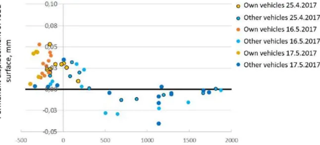
12 concrete layer in 2016. The thickness of the asphalt concrete layer was around 20 cm and the overall thickness of the structural layers of the embankment was about 1 m which lied on the peat subgrade. The roadway comprised oftwo 3.25 m wide lanes and narrow shoulders which was about 7.0 m in total width. The measurement tool at the test site included a five measurement probes monitoring temperature, dielectric value and electric conductivity at different levels from 0.25 m to 1.3 m below the roadway surface. In addition, two displacement transducers were installed below the outer wheel path of the lane from east to west direction. The transducers have been anchored into a stiff subgrade layer by using steel rods while the tips of the transducers were attached to the base of the asphalt layer, which rested against small steel plates. Fig. 2.6 shows the test site with the measurement tools. The loading test was in 2017,and the trucks had seven axles with total weight of 640 kN for each truck. During the loading test, the laser scanning and GPR measurement were under observation between the truck overruns.

A very interesting result was obtained from the distance of the wheel path from the point of displacement measurement. Fig. 2.7 shows the permanent displacements of road surface measured after each heavy vehicle overpass. The yellow dots indicate the permanent displacements caused by each overpass of the loading vehicles used for the study while the blue dots indicate the respective measurement results corresponding to other heavy vehicles that had passed over or nearby the displacement measurement point during the monitoring sessions.

(14)

13

Fig. 2.7 Permanent displacements of road surface measured for test truck and other vehicles (Pauli 2019).

The result from Fig. 2.7 shows that the rutting is continuously increasing due to the accumulating of the permanent displacement of the road surface when all vehicles are following the same wheel path by driving exactly above the measurement point. The rut development has levelled off due to the bouncing back of the road surface when the other vehicle passed around 0.5 to 1.5 far from the measurement point on the measurement site.

2.5.4 Malmvägen Test Site

Jonas (2019) set up a measurement to investigate the development of deformations on a test road with respect to the overpassing truck with a 5-axles and 22 tons of loading weight. The test roadway is constructed at Malmvägen 10 115 41 in Stockholm. The test road is built with BK2 standard, which is designed for 7000 vehicles per day, 3500 vehicles per direction. The length and width of the test roadway are 25m and 4m respectively. The 5-axle truck with 22 tonnes of payload was used as a vehicle to drive over the test road. The deformation measurements were done using a total station that scanned the roadway surface. The deformation development was evaluated according to the predetermined intervals on the number of crossing. A zero measurement of the roadway was made before the truck loading began to create a reference area. Then measurements were made at the following intervals: 10, 30, 70, 100, 140, 180, 220, 280, 360, 460 and 600 crossings. The time period of the measurements was made between 2019-06-18 and 2019-07-11.

The development of the total deformations is presented in Table 2.1, where the average values of the deformations are given.

Table 2.1 Average values of total deformations caused by number of truck passages (Jonas 2019).

Number of trucks passages 100 220 360 600

Total deformation [mm] 3 3 4 5

The development of the deformations on the road was less than expected. Since the truck did not drive in the same wheel path at each crossing, the road materials that were most tight to the sides of the wheels from

(15)

14 the previous crossing have been pushed back at the next crossing. Therefore, it is reasonable to assume the development of less deformation has occurred.

2.6 Summary of Previous Investigation

During recent years, road networks have been exposed to increasing stresses caused by axle load, spacing, weight, configurations and number of tires. This has been accompanied by the tendency to increase the total weight and length of trucks due to economic and environmental reasons. It has become an important debate on what would be the impacts on pavement deterioration.

This paper reviews the previous investigations related to roadway deterioration due to increased axle load to increase the knowledge and clarity of this research area for current and future researches.

Axle weights have a great effect on the remaining lifetime of a road. Increasing the total weight of heavy vehicles by Increasing the number of axles have an effect on road damages. Under several consecutive heavy loading, repetitions can lead to increased deformations and rutting speed, and in the worst case cause rapid plastic deformations. Moreover, weak subgrades dose not behave in a fully elastic fashion and because of this the deflections and deformations caused by a long vehicle combination does not have enough time to recover before the next consecutive axle loads at the same spot.

Using a narrow spacing in truck axle increases the road damage because the complete strain release does not happen between the load applications.

There are several and continuous developments that changes the condition of roadway pavements. These includes the increasing vehicle masses on roads, transition from dual tires to single tires in road transport and potential diminishment of the wheel path wander due to autonomous driving.

Results from Vesilahti test indicated that the peak values of vertical stresses of using single tires are about 30% higher than that of dual tire configuration. Therefore, the tire inflation pressure, which determines the size of the contact area between the tire and the road surface.

Inari test also revealed that, continuous cyclic loading and increasing the number of consecutive axles that resulting of heavier trucks or autonomous driving increases of road deterioration in wet and soft subgrade soil areas due to the impact of water pumping into the structural layers of the road.

From Highway 77 test, it can be inferred that the forthcoming introduction of autonomous vehicles and the rutting rate of the road surface will drastically increase if all the heavy vehicles are controlled by the same algorithms (follows exactly the same wheel path). Technology can make it possible to avoid this risk by enforcing the use of controlled algorithms of wheel path variation.

According to Malmvägen test, less deformation occurred than expected due to road materials that were most tight to the sides of the wheels from the previous crossing have been pushed back at the next crossing.

For upcoming and future measurement tests and studies:

It is important to determine the aim of the measurements. Is it to predict the deformation trend, to determine the roadway deterioration speed or to see how the underlying road infrastructure is affected especially if there are gas and water pipe or electricity extensions under the roadway.

For deformations measurements, it is preferable to install strain gauges into the road structure to be able to see which material layers are most affected. Moreover, displacement transducers and digital acceleration

(16)

15 transducers should be installed into the base course layer to monitor deflections under the truck wheels. In addition, GRP analysis and laser scanning for monitoring the road surface profile should be carried out.

In order to know how the infrastructure under the road is affected, similar infrastructure should be built under the test roadways. Also, deflection sensors and electrical conductivity should be installed into the road structure.

Study and determine a suitable method to avoid load repetitions on exactly the same wheel path in (2+1 roads), that is a specific category of three-lane road, consisting of two lanes in one direction and one lane in the other.

Finally, roadway spray seal or other materials can be used to reduce the pavement wear due to traffic load.

2.7 Linear Elastic Perfectly Plastic Model (Mohr Coulomb Model)

Elastoplastic soil means that all deformations are divided into elastic part, which is reversible portion and plastic part, which is irreversible part (Axelsson & Mattsson 2016). Fig. 2.8 shows the actual behaviour of the soil.

Fig. 2.8 Actual behaviour of elastoplastic soil (Axelsson & Mattsson 2016).

Fig 2.8 above shows that the soil would still deform plastically for small strains after unloading of the soil. The behaviour of the soil is complex and to simplify the soil behaviour, it is described as linear elastic and perfectly plastic (Knappett & Craig 2012). Fig. 2.9 shows the simplified behaviour of the soil.

(17)

16 Fig. 2.9 above shows that no deformation would be irreversible after unloading, as long as the shear stress does not exceed the shear stress in point Y’.

Mohr coulomb model is a linear elastic perfectly plastic model. The elastic part is depending on the isotropic elasticity of Hooke’s law. The plastic part is defined by the stress and strain, which is the yield function. The stress states illustrated by points. Points within the yield surface, all stresses are purely elastic, and all strains and deformations are reversible. Points which are outside the yield surface are perfectly plastic and the strains are irreversible. The yield functions are described by friction angle and cohesion and principal stresses (Plaxis 2019). Fig 2.10 shows the illustration of Mohr-Coulomb yield surface in principal stress space (C=0).

Fig.2.10 Mohr-Coulomb yield surface in principal stress space (Plaxis 2019).

2.8 Hardening Soil Model with Small Strain Stiffness

HS small model is a modification of the Hardening Soil model which that considered for increased stiffness of the soils at small strains. The advanced features of this model are most apparent in working load conditions. Also, the model gives more reliable displacements than other models. Using this model in the dynamic applications introduces hysteretic material damping. This model considers elastic in a very short strain range. When the strain amplitude is increasing, the soil stiffness is reducing nonlinearly. For an example for the stiffness-strain relation, Fig 2.8 show stiffness reduction curves (Plaxis 2019).

(18)

17 This reduction of soil stiffness correlated with loss of intermolecular and the forces of surface within the soil structure. The stiffness regains a heights recoverable value which is almost the same value of the initial soil stiffness, when the loading direction is reversed (Plaxis 2019).

According to Masing in 1926, the rules description of the hysteretic behaviour of soil materials in the cycles of unloading and reloading illustrated in Fig. 2.9 and stated in the following:

• Once unloading, the shear modulus is similar to the initial tangent modulus for the initial loading curve.

• The unloading – loading curves shape is similar to the initial loading curve but in double of size.

Fig. 2.9 Hysteretic material behaviour (Plaxis 2019).

Masing’s rule has been adopted in this model with an increase of the plastic stiffness during the cycles. Stiffness will be in the original range at the beginning of each loading. but the stiffness will decrease in a non-linear way when the stiffness decreases. In the sequential cycles, the stiffness is higher than in the original loading. In addition, during the initial loading, the stiffness reduces more rapidly within the cycle than in the rest of the cycles. Fig. 2.10 show the loading – unloading materials behaviour.

(19)

18

2.9 UBCSAND Model

UBCSAND is a 2D model developed by Puebla, Byrne and Phillips in 1997 at University of British Columbia, which the model name came from (UBC). The model is formulated based on the classical plasticity theory with a hyperbolic strain hardening rule. The model specifically used the plastic hardening count on the principle of strain hardening. The hardening rule links the mobilised friction angle to the plastic shear strain at a given stress. Fig. 2.11 shows the original UBCSAND hardening rule. The model includes a 2D Mohr Coulomb yield surface and an identical unrelated plastic potential function (Plaxis 2019).

Fig. 2.11 Original UBCSAND hardening rule (Plaxis 2019).

The model has been justified in several applications related to liquefaction. The hysteric response of sand under cyclic loading in the model is captured in a simplified method. Therefore, the model can be used to predict the unload and reload cycles in more accurately. UBCSAND model can be used in dynamic loading cases due to the features of exhaustive loading and unloading for dynamic loading (Puebla 1999).

According to Mujtaba et al in 2017, the SPT-N could be calculated form friction angle relation. See Eq.3 for the rest of material parameters see Eq. 4, 5, 6 and 7.

ᵠ = (20 × (𝑁1₎

60)0.5+ 20 (3)

𝐾_𝐺∗𝑒= 21.7 × 20 × (𝑁₁)₆₀0.3333 (4)

𝐾_𝐵∗𝑒 = 𝐾_𝐺∗𝑒× 0.7 (5)

𝐾_𝐺∗𝑝 = 𝐾_𝐺∗𝑒× 20 × (𝑁₁)₆₀2 × 0.003 + 100 (6)

(20)

19 ᵠ𝑝= ᵠ𝑐𝑣+ (𝑁₁)60 10 + max (0; (𝑁₁)60− 15 5 ) (7)

According to Hamidi et al in 2009, the constant volume friction angle could be calculated from the maximum friction angle relation. See Eq. 8

ᵠ𝑚𝑎𝑥 = ᵠ𝑐𝑣+ 0.8 𝛹𝑚𝑎𝑥 ₍₈₎

2.10 Aim and Objectives

As mentioned, there are several studies presents problem with the roadway embankment system that can be most likely caused by traffic loading. But in the lack of focused studies on cyclic loading in flexible pavement embankment with water pipelines, this study is the preface of a more detailed investigation and study of how the changing of wheel path loading effect the deformation behavior comparing with the using of the same wheel path of the roadway embankment. The purpose with this master thesis is to analyze the cycling loading of a 500 on the roadway embankment and the water pipelines induced by five-axles truck with a numerical software, PLAXIS 2D, and to increase the knowledge of axle load accumulations. The established objectives are:

• Model a flexible roadway and three water pipelines under the road embankment in Plaxis 2D. • Understand some of the main parameters that influence the cyclic and dynamic loading.

• Analyze the stress – deformation behavior, and the developed failure mechanisms and stresses conditions around the water pipelines.

• Compare three different material models under 500 cycles. • Compare with different wheel path loading under 500 cycles.

• Compare two different axle loads and gross vehicle weight under 500 cycles. • Compare two different truck speed under 500 cycles.

• Compare two models with different flow conditions with and without water table level. • Compare two different truck standards.

(21)

20

Methodology

Plaxis 2D has been used to analyse the deformation behaviour in the roadway embankment. Plaxis 2D is a two-dimensional finite element which models and simulate the soil behaviour. The software used form stability, deformation and groundwater flow analysing in geotechnical engineering (Brinkgreve et al. 2017).

3.1 Road Design

The roadway consists of road embankment layers and water pipelines under the embankment.

3.1.1 Design of Road Embankment

Flexible pavement road with two-lanes has been used in this research. The road width is 4m for one way with a 1:3 slope according to (TRV Geo 2011). Fig. 3.1 shows the roadway embankment dimensions.

Fig.3.1 Road embankment cross-section.

The flexible roadway superstructure was assumed to be of gravel bitumen superstructure (GBÖ) (TRV 2011). The layers’ dimensions and materials of the superstructure are illustrated in figure 3.2.

Fig. 3.2 GBÖ superstructure layers (TRV 2011).

The road embankment consists of three main layers, 0.15m of Asphalt, 0,08m of Base (crushed stone) and 0.42m of Sub-Base (crushed stone) lying on 15m of Subgrade (Sand).

(22)

21 3.1.2 Design of Water Pipelines

Three water pipelines under the road embankment has been used in this project. The pipelines design stander is (Principritning CBB.311) according to (AMA Anläggning17 2017). Fig. 3.3 shows the water pipelines depth and dimensions for the specific road in this project.

Fig. 3.3 Pipelines cross-section under road embankment according to (AMA Anläggning 2017).

The water pipelines made of PVC material with 10mm of wall thickness. From Fig 3.3 above: pipe with green (D) is a 400mm rainwater drainage pipe, pipe with red (S) is a 200mm wastewater pipe and pipe with blue (V) is a 160mm drinking water pipe.

3.2 Material Parameters

3.2.1 Material Parameters of Road Layers

Three different material models have been used in this project. The layers properties and parameters are according to (Hüseyin et al. 2018). Some parameters have been medicated to be suitable with the specific roadway in this project.

The material parameters for the three different material models are under (3.5.1 Different Material Models) in tables 3.3, 3.4 and 3.5.

(23)

22 3.2.2 Material Parameters of Water Pipelines

The pipes have been model as plate element in Plaxis 2D software. The pipelines Young’s Modulus is according to (Suleiman 2002), which the PVC pipe stiffness, E equal to 2,756,000 KN/m3. In addition, the unit weight of the PVC pipe is around 13.7 KN/m3 and 10mm wall thickness. Therefore, the pipe parameters have been calculated from the follow equations. See Eq. 9, 10, 11 and 12.

𝐸𝐴 = 𝐸 × 𝐵 × 𝐻 (9) 𝐸𝐼 = 𝐸 × 𝐵 ×𝐻3 12 (10) Where H = Thickness (d) B = 1 ml 𝐷𝑒𝑞= √ 12𝐸𝐼 𝐸𝐴 (11)

Where Deq Equivalent thickness

𝑊 = γ × 𝑑 (12)

Where W Weight of plate

The calculated parameters for the pipes are shown in Table. 3.1.

Table 3.1 Pipe parameters.

The interaction between the pipe wall and the soil is modelled at the external pipe boundary by means of interfaces. The interfaces allow for the specification of a reduced wall friction compared to the friction in the soil (Plaxis 2019).

An interface has been created for assigning a compliant boundary condition with an assumed Strength reduction factor inter, Rinter equal to 0.7.

3.3 Model Design

A full cross-section of flexible roadway embankment with water pipelines were modelled with the Plaxis software. The section consisted asphalt bitumen layer above base and subbase of crushed stone that rested on a subgrade layer of sand.

The truck consists of 5 axels with single wheel of each axel. The axle load is supposed to be divided equally into both wheels of the axle. A line load is distributed on top of the plate which is supposed to illustrate the behaviour of the wheels load. The line load is equal to the wheel width. The water table level is assumed to

Material Unit PVC

Set Type Plate

Normal Rigidity Stiffness, EA KN/m 27560

Flexional Rigidity Stiffness, EI KN/m2/m 0.23

Equivalent Thickness, d m 0.01

Specific Weight, W KN/m/m 0.137

(24)

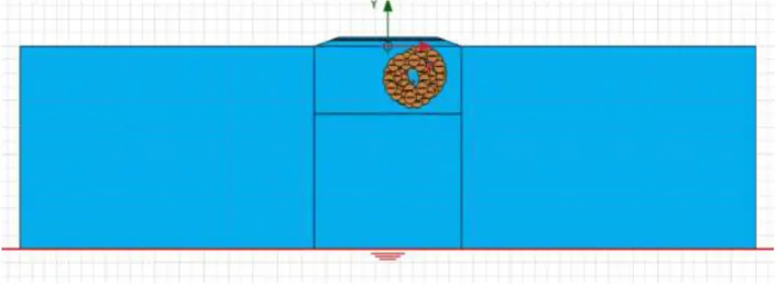
23 be under the road embankment. Fig 3.4 and 3.5 shows the original model of simplified cross-section of the roadway.

Fig.3.4 Original geometry of the model.

Fig. 3.5 Original geometry of road embankment.

From Fig 3.5 the road layers are shown as asphalt is black, base is yellow, subbase is brown and subgrade is silver.

The truck axle was assumed to be 10 tons for each axle and the load assumed to be divided into 5 tons for each wheel. line load with green express wheel load which is assumed to 5 tons. this gives the truck a gross vehicle weight of 50 ton. The width of line load is 0.385m equal to the wheel width and the distance between the both lines load is 2.2m from centre to centre as the distance between the truck wheels. Each line load equal to 127.4 kN/m which is (5ton × 9.81N/kg / 0.385m).

(25)

24 The model was meshed with a fine element distribution with15 nodes. A coarseness factor has been applied with 0.75 around the subgrade boundaries and with 0.5 around the embankment layers. Fig 3.6 shows the mesh of the model.

Fig. 3.6 Mesh element of the model.

Refined mesh areas marked with different shades of green. Lighter shades are more refined. The mesh was generated, and the quality of the mesh was not good enough, so more refine mesh has been applied to the layer embankment until the mesh quality became good, so the models were able to be computed. Fig. 3.7 shows the mesh quality.

(26)

25

3.4 Model Procedure

When the modelling was done, the initial state had to be calculated. This could be done by generation the initial effective stresses with K0 producer and by a phreatic pore pressure calculation, for the initial soil (subgrade / sand). Then the pipelines were created in the next construction phase under plastic loading. After that, each layer of the embankment created in separated construction phase from subbase to asphalt under plastic loading type of calculation. All deformation created during these phases were reset before the cyclic loading calculation.

To illustrate the behaviour of cyclic loading from the truck, a calculating phase was used for each loading and unloading from the truck wheels axles

This phase was a dynamic with consolidation loading under a given dynamic time interval, which is the loading, unloading and consolidation of each truck cycle. This type of loading was used to let the road layers subjected to the cyclic loading and to consolidate before subjected to loading again by the next truck.

3.4.1 Phases Construction

Since the truck consists of five axles with a single wheel of each. The time between the axles varies depending on the distance between the axles. Therefore, repeating the same phase for five hundred times illustrated the five hundred trucks. The time interval between each truck is two seconds. Fig. 3.8 shows the truck dimensions that have been used in the model.

(27)

26 Therefore, five hundred and five phases were needed for five hundred cycles, and they are:

• Initial phase, K0 producer.

• Phase 1: Pipelines construction, plastic loading. • Phase 2: Subbase construction, plastic loading. • Phase 3: Base construction, plastic loading. • Phase 4: Asphalt construction, plastic loading.

• Phase 5: One cycle, dynamic and consolidation loading.

Phase number 5 was repeated five hundred times and illustrated therefore a total of 500 trucks as a total of 505 phases.

3.4.2 Time Calculation

Time for loading, unloading and consolidation. Each wheel is assumed to load the embankment periodical with a sinus shape. See Eq. 7.

𝑞(𝑡) = 𝐿 𝑠𝑖𝑛 (𝜔𝑡) (6)

Where q(t) The time dependent load that is acting on the embankment L Traffic load for each wheel (5 ton)

𝜔 Angular frequency/ circular frequency of the wheel. t Time

To calculate the circular frequency of the wheel, the circumference of the wheel and speed of the track are needed. The wheel circumference is 3.34m and the maximum truck speed is b 50km/h. See Eq. 7, 8 and 9.

𝑅𝑃𝑀 =𝑇𝑟𝑢𝑐𝑘 𝑆𝑝𝑒𝑒𝑑 (𝑐𝑚/𝑚𝑖𝑛)

𝐶𝑖𝑟𝑐𝑢𝑚𝑓𝑒𝑟𝑒𝑛𝑐𝑒 (𝑐𝑚) (7)

Where RPM Revolution Per Minutes

=83333.33

334 = 249.5 𝑅𝑃𝑀

𝑓 =𝑅𝑃𝑀

60 (8)

Where f Oscillation frequency

𝑓 =249.5

60 = 4.158 ℎ𝑒𝑟𝑡𝑧

𝜔 = 2𝜋 𝑓 (9) 𝜔 = 2𝜋 × 4.158 = 26.125 𝑟𝑎𝑑/𝑠

(28)

27 Fig 3.9 shows the sinus curve. It is though only the first part of the sinus curve that is loading and unloading the embankment.

Fig. 3.9 Illustration of loading and unloading for the wheel.

The time it takes for the wheel to load the road embankment is the same as the unloading time of the wheel, and the time is calculated to 0.06 seconds. The full load is applied when the centre of the wheel is above the determined point, this phase is where loading changes to unloading.

Each wheel is loading and unloading the road embankment, therefore the time between each wheel is needed. The distance between the wheels is showing in Fig. 3.8. The time between each wheel have been calculated by using Eq. 10.

Where [0.06 × 2] The unloading time for first wheel and the loading time for second wheel. The time between each wheel of the truck showing in Table 3.2.

Table 3.2 The time between each wheel of the truck. 𝑡 =𝐷𝑖𝑠𝑡𝑎𝑛𝑐𝑒 𝑏𝑒𝑡𝑤𝑒𝑒𝑛 𝑡𝑤𝑜 𝑤ℎ𝑒𝑒𝑙𝑠 (𝑚)

𝑇𝑟𝑢𝑐𝑘 𝑆𝑝𝑒𝑒𝑑 (𝑚/𝑠) − [0.06 × 2] (𝑠) (10)

Distance between Distance (m) Time between (s)

First wheel to Second wheel 1.995 0.02365

Second wheel to Third wheel 2.605 0.06757

Third wheel to Fourth wheel 1.370 - 0.02135

Fourth wheel to Fifth wheel 1.380 - 0.02063

(29)

28 Fig. 3.10 shows the calculated loading curves of the wheels truck.

Fig. 3.10 Loading and unloading of one truck.

3.5 Model Differences

As mentioned in 2.10 Aim and Objectives, the original model was changed to be compared with different material models, truck speeds, axle loads, water flow level and wheel path loading.

3.5.1 Different Material Models

Three different material models have been analysed in this project. To see how the changing of the material model will affect the road deformation. Mohr coulomb model, hardening soil model with small strain stiffness and UBCSAND model. The definition and theoretical part of the three models were written in the background chapter 2.7, 2.8 and 2.9. The material properties are according to (Hüseyin et al. 2018). Tables 3.3, 3.4 and 3.5 shows the material parameters for each model.

Table 3.3 Material parameters for Mohr coulomb model.

Material Asphalt Base (Crushed Stone) Sub-base (Crushed Stone) Sub-grade (Sand)

Model Linear elastic Mohr Coulomb Mohr Coulomb Mohr Coulomb

Thickness (m) 0.150 0.080 0.42 15

Young’s modulus (KN/m2₎ _4500×103 _506.7×103 _166.7×103 _150×103

Poisson’s ratio 0.35 0.35 0.35 0.3

Dry unit weight (KN/m3₎ ₂₄ _21.65 _21.65 ₁₈

Cohesion (KN/m2₎ _- ₀ ₀ ₀

Friction angle (degree) - 40 40 35

(30)

29

Table 3.4 Material parameters hardening soil model with small strain stiffness.

Table 3.5 Material parameters for UBCSAND model.

Material Unit Asphalt _{(Crushed Stone)}Base _{(Crushed Stone)}Sub-base Sub-grade _(Sand)

Model Linear elastic HSsmall HSsmall HSsmall

Thickness m 0.150 0.080 0.42 15

Young’s modulus, E KN/m2 _4500.103

Secant stiffness, E50ref KN/m2 260.103 100.103 55.103

Tangent stiffness, Eoedref KN/m2 235.103 90.103 55.103

Unloading reloading stiffness, Eurref KN/m2 608.103 200.103 180.103

Poisson’s Ratio, ν 0.35 0.35 0.35 0.3

Surface shear modulus, G0ref KN/m2 255.103 110.103 65.103

Shear strain, 𝛄𝟎.𝟕 5.10-6 5.10-6 2.10-4

Power, m 0.7 0.7 0.6

Dry unit weight, 𝛄 KN/m3 ₂₄ _21.65 _21.65 ₁₈

Cohesion, C KN/m2 ₀ ₀ ₀

Friction angle, ϕ degree 40 40 35

Dilation, Ψ degree 10 5 5

Material Unit Asphalt _{(Crushed Stone)}Base _{(Crushed Stone)}Sub-base Sub-grade _(Sand)

Model Linear elastic UBCSAND UBCSAND UBCSAND

Thickness m 0.150 0.080 0.42 20

Young’s modulus, E KN/m2 _4500.103

Poisson’s Ratio, ν 0.35

Dry unit weight, 𝛄 KN/m3 ₂₄

K* Be 824.56 824.56 680.68 K* Ge 1177.94 1177.94 972.4 K* Gp 1513.53 1513.53 469.2 me 0.5 0.5 0.5 ne 0.5 0.5 0.5 np 0.5 0.5 0.5 ᵠcv degree 32 36 31 ᵠP degree 35 39 33.125 Cohesion, C KN/m2 ₀ ₀ ₀ σt KN/m2 0 0 0 (N1)60 20 20 11.25

(31)

30 For the rest of the model differences, UBCSAND model was used as a material model.

3.5.2 Different Truck Speeds

As mentioned above, the truck speed was 50km/h which is the maximum speed. So, another speed has been used to see how the truck speed or velocity will affect the road deformation. Therefore, truck speed with 30km/h was used in the model. Same equations have been used for time calculation of loading, unloading and consolidation. Se Eq. 6, 7, 8 and 9.

Fig 3.11 shows the sinus curve. It is though only the first part of the sinus curve that is loading and unloading the embankment.

Fig. 3.11 Illustration of loading and unloading for the wheel.

The time it takes for the wheel to load the road embankment is the same as the unloading time of the wheel, and the time is calculated to 0.1 seconds. The full load is applied when the centre of the wheel is above the determined point, this phase is where loading changes to unloading.

The time between each wheel have been calculated by using Eq.10. The time between each wheel of the truck showing in Table 3.6.

Table 3.6 The time between each wheel of the truck.

Second wheel to Third wheel 2.605 0.1126

Third wheel to Fourth wheel 1.370 -0.0356

Fourth wheel to Fifth wheel 1.380 -0.0344

(32)

31 Fig. 3.12 shows the calculated loading curves of the wheels truck.

Fig. 3.12 Loading and unloading of one truck.

3.5.3 Different Axel Loads and Gross Vehicle Weight

As mentioned before, the axle load of the truck was 10 tons which assumed to be 5 tons for each wheel. So, another axle load has been used to see how the increasing of axle load will affect the road deformation. Therefore, axle load with 12 tons was used in the model. Which is assumed to be 6 tons for each wheel. Which this gives the truck a gross vehicle weight of 60 ton. Each line load will increase to be equal to 164.4 kN/m which is (6ton × 9.81N/kg / 0.385m).

3.5.4 Different Water Flow Level

As aforementioned, the water table level was assumed to be under the road embankment. So, another model has been analysed without water level to see how the water table affect the subgrade soil layer around the pipelines and how will affect the road embankment deformation. Fig. 3.13 shows the water table level under the subgrade layer.

(33)

32 3.5.5 Different Wheel Path Loading

A different wheel path loading has been used in the model to see how it will affect the road deterioration and to compare with the same wheel path loading as in autonomous vehicles. Therefore, three phases with three different wheel path were used in the model to illustrate the random wheel path passing of the truck. First Phase is the same wheel pass loading as the original model. Fig. 3.14 shows the first wheel path loading.

Fig. 3.14 First wheel pass.

Second phase is when the truck passing to the right beside the previous wheel path. Fig. 3.15 shows the second wheel path loading.

(34)

33 Third phase is when the truck passing to the left beside the first wheel path. Fig. 3.16 shows the second wheel path loading.

Fig. 3.16 Third wheel path.

Therefore, these three phases have been repeated randomly for the 500 cycles.

3.5.6 Different Truck Standards

A new different truck standard has been used in the model to see how using different wheelbase (WB) will affect the road deterioration and to compare between the different standards. The new truck consists of four axles with a single wheel of each. Fig. 3.17 shows the new truck dimensions that have been used in the model. WB = 5.618m according to Volvo Truck Corporation (Modellutbud).

(35)

34 The axle loads equal to 8 tons for each axle which have a gross vehicle weight of 32 ton. The time it takes for the wheel to load and unload the road embankment is the same as the five axles truck (Volvo X-PRO Truck). The time between each wheel of the truck showing in Table 3.7.

Table 3.7 The time between each wheel of the truck.

Fig. 3.18 shows the calculated loading curves of the wheels truck.

Fig. 3.18 Loading and unloading of the new truck.

Result and Discussion

After inputting soil, vehicle, pipelines and superstructure parameters. The roadway deformation was performed in Plaxis 2D software. More results that are not presented in the report can be found in Appendix A, B, C, D and E. All results needed for following the analysis are presented in the report.

Second wheel to Third wheel 1.370 - 0.02135

Third wheel to Fourth wheel 1.380 - 0.02063

(36)

35

4.1 Difference Between the Models

Three different material models were used in this research. Mohr coulomb model, hardening soil model with small strain stiffness, and UBCSAND model. The result of vertical deformation after one cycle of the truck is shown respectively in the figures below. See Fig. 4.1, 4.2 and 4.3.

Fig. 4.1 Total displacement after one cycle of the truck for Mohr coulomb model.

(37)

36

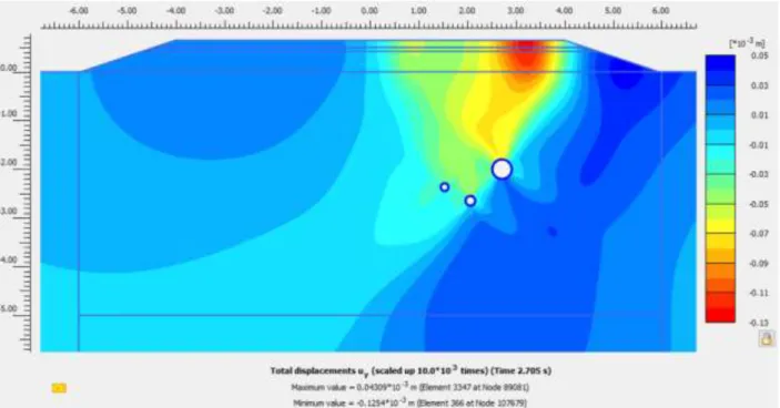
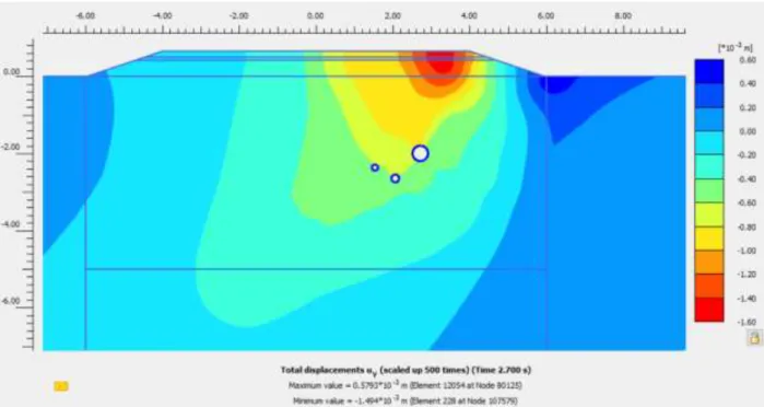
Fig. 4.3 Total displacement after one cycle of the truck for UBCSAND model.

The result shows that UBCSAND model has the highest settlement and heaving result by around (-1.5mm) under the wheels passing and (+0.5mm) at the end of the road slope. Hardening soil model with small strain stiffness comes second by around 1.16mm) and (+0.33mm). Then Mohr coulomb model by around (-0.13mm) and (+0.04mm). The difference may not be that large, but these differences are just after one cycle. Therefore Fig. 4.4, 4.5 and 4.6 shows the deformation after 500 cycles.

(38)

37

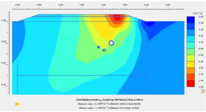
Fig. 4.5 Total displacement after 500 cycles of the truck for hardening soil model with small strain stiffness.

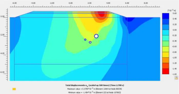
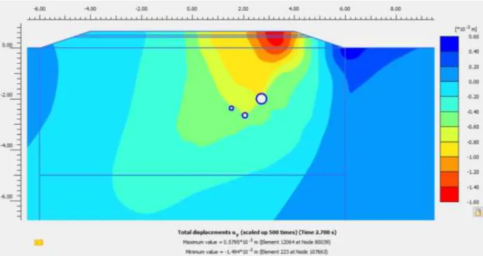
Fig. 4.6 Total displacement after 500 cycles of the truck for UBCSAND model.

Table 4.1 shows the result of settlement and heaving of the roadway after 500 cycles of the truck for the three models.

(39)

38

Table 4.1 Result of settlement and heaving of the roadway after 500 cycles of the truck for three different models.

Material Model Maximum displacement (Heaving) (mm)

Minimum displacement (Settlement) (mm)

Mohr coulomb 0.04 0.15

HSs 17 18

UBCSAND 38.5 44

4.2 Difference Between the Speeds

Two different truck speed was used in this research which are 50 km/h and 30 km/h with using of UBCSAND model. The result of vertical deformation after one cycle of the truck is shown respectively in the figures below. See Fig. 4.7 and 4.8.

(40)

39

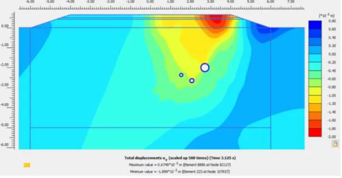
Fig. 4.8 Total displacement after one cycle of the truck for 30 km/h speed.

The result shows that after one cycle of the truck, the truck with a speed of 50 km/h has a displacement (- 1.5mm) and (+0.58mm) while the truck with a speed of 30 km/h has (-1.9mm) and (0.68mm). Therefore, the result shows that after one cycle, the highest speed has less deformation. Fig 4.9 and 4.10 shows the deformation after 500 cycles of the truck.

(41)

40

Fig. 4.10 Total displacement after 500 cycles of the truck for 30 km/h speed.

The result shows that the highest truck speed (50km/h) has the highest settlement and heaving result by around (-38mm) under the wheels passing and (+44mm) at the end of the road slope. While the lower speed (30km/h) has around (-20mm) and (+20mm). Therefore, the result indicates that with increasing the number of cycles, the lower speed produces less deformation on the roadway layers.

4.3 Difference Between the Axle Loads

Two different Axle loads were used in this test, which are10 tons and 12 tons with using of UBCSAND model. The result of vertical deformation after one cycle of the truck is shown respectively in the figures below. See Fig. 4.11 and 4.12.

(42)

41

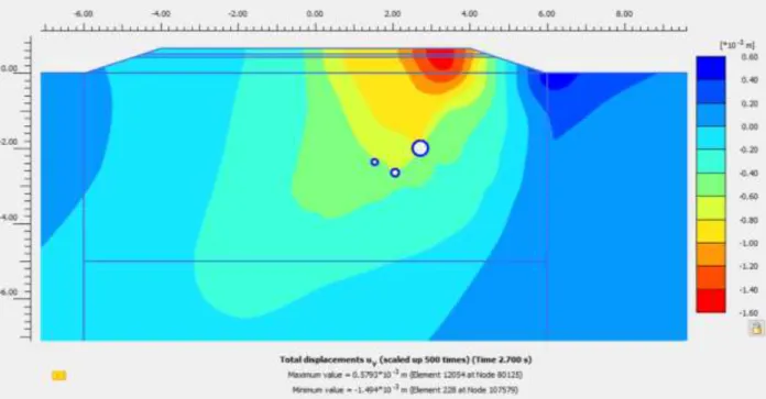
Fig. 4.11 Total displacement after one cycle of the truck for 10 tons load for each axle.

Fig. 4.12 Total displacement after one cycle of the truck for 1 ton’s load for each axle.

The result shows that after one cycle of the truck, the truck with axle load of 10 tones has a displacement (- 1.5mm) and (+0.58mm) while the truck with axle load of 12 tons has (-2.2mm) and (+1mm). Therefore, the result shows that after one cycle, the heavier axle load has higher deformation. Fig 4.13 and 4.14 shows the deformation after 500 cycles of the truck.

(43)

42

Fig. 4.13 Total displacement after 500 cycles of the truck for 10 ton’s loads for each axle.

Fig. 4.14 Total displacement after 500 cycles of the truck for 12 tons load for each axle.

The result shows that the heavier truck axle load (12 tons) has a slightly high settlement and heaving by around (-45mm) under the wheels passing and (+45mm) at the end of the road slope. While the lightest truck axle load (10 tons) has around ((-38mm) and (+44mm). Therefore, result indicates that with increasing the axle load of the truck, the heavier truck produces slightly higher deformation on the roadway layers.

(44)

43

4.4 Difference Between the Water Flow Level

Two different water flow level were used in this study, which are at under the road embankment (0m) and at -15m of the road embankment with using of UBCSAND model. The result of vertical deformation after one cycle of the truck is shown respectively in the figures below. See Fig. 4.15 and 4.16.

Fig. 4.15 Total displacement after one cycle of the truck when the water level below the road embankment.

(45)

44 The result shows that after one cycle of the truck, model with the lower water flow level has a displacement 0.8mm) and (+0.17mm) while the model with higher water flow level under the road embankment has (-1.5mm) and (+0.58mm). Therefore, the result shows that after one cycle, the model with the lower water level has lower deformation on the roadway layers. Fig 4.17 and 4.18 shows the deformation after 500 cycles of the truck.

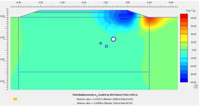
Fig. 4.17 Total displacement after 500 cycles of the truck when the water level below the road embankment.

(46)

45 The result shows that the model with lower water flow level (-15m) has a Significant less settlement and heaving by around (-0.01mm) under the wheels passing and (+0.13mm) at the end of the road slope. While the model with higher water flow level (0m) has around ((-38mm) and (+44mm). Therefore, the result indicates that with the reduction of the water flow level the roadway embankment deformation was reduced.

4.5 Difference Between the Wheel Path Loading

Two different wheel path loading were used in this study, which are at same and randomly different wheel path loading on the road embankment with using of UBCSAND model. The result of vertical deformation after one cycle of the truck is shown respectively in the figures below. See Fig. 4.19 and 4.20.

(47)

46

Fig. 4.20 Total displacement after one cycle of the truck for different wheel path loading.

The result shows that after one cycle of the truck, model with same wheel path loading has a displacement (-1.5mm) and (+0.58mm) while the model with different wheel path loading has (-1.5mm) and (+0.58mm). Therefore, the result shows that after one cycle, the models with same and different wheel path loading have the same deformation amount on the roadway layers. Fig 4.21 and 4.22 shows the deformation after 500 cycles of the truck.

(48)

47

Fig. 4.22 Total displacement after 500 cycles of the truck for different wheel path loading.

The result shows that the truck with the same wheel path loading has almost the same settlement and higher heaving by around (-38.5mm) under the wheels passing and (+44mm) at the end of the road slope. While the truck with different wheel path loading has around ((-39mm) and (+37mm). Therefore, result indicates that with different wheel path loading of the truck produces lower deformation (heaving) on the roadway slope surface.

4.6 Difference Between the Standards of Trucks

Two different truck standards were used in this study, which are truck with 5 axles and truck with four axles with using of UBCSAND model. The result of vertical deformation after one cycle of the truck is shown respectively in the figures below. See Fig. 4.23 and 4.24.

(49)

48

Fig. 4.24 Total displacement after one cycles of the truck for the new standard of the truck (four axels).

The result shows that after one cycle of the truck, truck with five axles wheel has a displacement (-1.5mm) and (+0.58mm) while the model with four axles truck has (-1.34mm) and (+0.5mm). Therefore, the result shows that after one cycle, the truck with five axle has higher deformation on the roadway layers. Fig 4.25 and 4.26 shows the deformation after 500 cycles of the truck.

(50)

49

Fig. 4.26 Total displacement after 500 cycles of the truck for the new standard of the truck (four axles).

The result shows that the truck with five axles has almost higher settlement by around (-38.5mm) under the wheels passing and lower heaving by (+44mm) at the end of the road slope. While the truck with four axles has around ((-33mm) and (+47mm). Therefore, result indicates that the truck with five axles produces lower deformation (heaving) on the roadway slope surface.

4.7 Pipeline Axial Force

Table 4.2 shows the amount of axial force that acting on the pipe due to truck loading. See Appendix A for more details.

Table 4.2 Axial force on the pipeline after 500 cycles.

Differences Axial Force (kN/m)

Maximum Minimum Material Model Mohr Coulomb -2.4 -3.6 HSs -5.8 -8.4 UBCSAND -4.25 -6 Truck Speed 50 km/h -4.25 -6 30 km/h -9.8 -10.7

Axle Load 10 tones -4.25 -6

12 tones -4.6 -6

Water Level Under road embankment -4.25 -6

-15m 1.86 -3.17

Wheel Path Loading Same -4.25 -6

Different -4.45 -6.5

Truck Standard

5 Axels -4.25 -6

4 Axels -4.83 -6.22

The result shows that the UBCSAND model has less axial force than HSs model on the pipe. The reducing of truck speed increases the axial force by around 40%. The increasing of the axle load does not have a real

(51)

50 effect on the increasing axial force. Reducing the water flow level has a great effect on axial force reduction. The use of different wheel path loading produces slightly higher axial force more than using the same wheel path loading. Reducing the number of axles led to increased axle force.

Conclusion and Future Work

5.1 Conclusion

The aim of this thesis has been to analyze the deterioration and deformation, induced by 5-axles truck, in the road embankment with a numerical software, PLAXIS2D, and to increase the knowledge of axle load accumulations. The following conclusions were drawn.

The development and accumulation of truck axle load in this thesis could be seen with the help of the different created models. The result indicates that:

• UBCSAND model is the most suitable material model with the cyclic loading cases, which has the highest deformation.

• As the number of cycles increases, the truck with lower speed produces less deformation on the roadway layers.

• The truck with a heavier axle load has higher deformation.

• As the level of water flow decreases, the deformation of the road embankment is reduced.

• The truck with different wheel path loading produces lower deformation (heaving) on the roadway slope surface.

• The truck with five axles standard produces lower deformation (heaving) and higher (settlement) on the roadway slope surface.

• As the truck speed decreases, the axial force on the pipelines increases.

• As the level of water flow decreases, the axial force on the pipelines decreases.

The results are reasonable and therefore, the modeling presented in this thesis can be used to give a forecast of the problems related to the increased axle load and cyclic loading. 2.6 shows the summary of previous investigation.

5.2 Future Work

Since this is the first approach to the problem, further investigation has to be done. Physical experiments can be performed as well as data collection from real sites.

An interesting point for further work is to look from a perspective where we should transport X amount of sand from A to B. So, different gross vehicles weight has different cycles. Also, the models can be tested with Different road slope angles in order to see how the slope angles affect road deterioration.

The regular trucks in Stockholm the standard truck is 3-axle with approximate 25 tons gross weight. this gives 8.33 ton on each axle. would be interesting to calculated with these load cases.

In this report the roadway was loaded with 500 cycles, to further investigate the road deterioration, would be interesting to see the situation at a bigger number of cycles.

(52)

51

References

Department of Transport in South Africa (1997) The Damaging of Overloaded Heavy Vehicles on Roads. CSIR, Roads and Transport Technology Report. Fourth edition.

Puebla, H. (1999). A constitutive model for sand analysis of the CANLEX embankment, PhD Thesis, University of British Columbia, Vancouver, Canada.

Ministry of Works (2000) Axle Load Surveys. Transport & Communications, Roads Department Report. Gaborone, Botswana.

BWIM-mätningar (2002 och 2003) Slutrapport. VV Publication 2003:165.

BWIM-mätningar (2004 och 2005) Projektrapport. VV Publication 2006:136.

ATB VÄG (2005) VV Publication 2005:112.

Mattias Hjort, Mattias Haraldsson, Jan M. Jansen (2008) Road wear from Heavy Vehicles – an overview. NVF committee Vehicles and Transports Report. Borlänge, Sweden.

COST 334 (2011) Effects of Wide Single Tyres and Dual Tyres. Report, Chapter 4, version 29.

Knappett, J.A., & Craig, F. (2012). Craig’s Soil Mechanics (8 ed.). New York: Spon Press.

David Huft (2014) Truck Axle Configuration Effect on Roads. DOT, Connecting South Dakota and the Nation.

Petri Varin, Timo Saarenketo (2014). Effect of Axle and Tire Configurations on Pavement Durability. ROADEX Network Report.

Dave Stevens, Graham Salt (2015) Effects of Increased Axle Loadings on Local Roads. GeoSolve Pavements Group.

Pauli Kolisoja, Antti Kalliainen, Ville Haakana (2015) Effect of tire configuration on the performance of a Low Volume Road exposed to heavy axle loads – response measurements, Transportation Research Record 2474, pp. 166 – 173. DOI: 10.3141/2474-20.

Axelsson, K., & Mattsson, H. (2016). Geoteknik. Lund: Studentlitteratur AB.

Volkan Emre Uz, Mehmet Saltan, Islam Gökalp (2016). Feasibility of Using 4th Power Law in Design of Plastic Deformation Resistant Low Volume Roads. Procedia Engineering.

AMA Anläggning 17. (2017). Allmän material- och arbetsbeskrivning för anläggningsarbeten.

Hüseyin Karatağ, Seyhan Firat and Nihat Sinan Işik. (2018). Evaluation of Flexible Highway Embankment Under Repetitive Wheel Loading Using Finite Element Analysis.