Application of the Cowell Index to Monthly Streamflow Analysis
Robert T Milhous1Hydrologist, Torries Peak Analysis Fort Collins, Colorado 80526
Abstract. Temporal patterns of streamflows are important in the fluctuating physical and
biological environment of rivers. Colwell proposed two measures of predictability: constancy, and contingency. The measures are based on the mathematics of information theory. The Colwell Index, predictability, is the sum of the two measures. A consistent method of calculating the Colwell Index for monthly streamflows data was developed and is 1) use monthly discharge time steps, 2) uses 12 discharge classes with the 12th class being all monthly discharges larger than the
11th class boundary, 3) use the equation B(i) = 0.015625 (2)α Q
m where α = i-1 from i = 1, 2, ,11
and Qm is a reference discharge to define the discharge class boundaries, 4) use the median monthly
discharge as the reference discharge. The Colwell Indices for eight rivers are presented. The rivers were selected because they show the variation in the index that is possible. The eight rivers
represent a wide range of watershed types and climates. The range of the Colwell Index for the eight rivers was from 0.21 to 0.84, of consistency 0.10-0.46 and of contingency 0.09-0.44. The contingency is a measure of the seasonal predictability of streamflows. The Gunnison River in Colorado has three periods with difference in the water management. The Cowell Indices was calculated for each of the periods. The consistence increased in all three periods but the contingency was reduced. The principle value of the Colwell Index is in making comparisons, between rivers and water management actions, of the uncertainty of the variable stream
environments. This ability to use one index to make a comparison of uncertainty may make the Colwell Index a valuable tool in the analysis of environmental flow needs.
1. Introduction
Temporal patterns in fluctuating physical and biological phenomena are of interest in several fields of biology because of their importance as evolutionary constraints (Colwell, 1974). Colwell proposed two ‘simple’ measures of predictability: constancy, and
contingency. Predictability is the sum of the two measures. The measures were expected by Colwell ‘to clarify and simplify the wide variety of terms used to describe aspects of temporal pattern’. According to Colwell the measures are based on the mathematics of information theory. In fact, the measures are not simple and are difficult to place in prospective. This paper attempts to show how the measures might be calculated using monthly streamflows and what they might show about variation between rivers and between water management actions. Poff and Ward (1989) used the index in a paper on understanding hydrology as a variable in the aquatic ecosystem. Thoms and Sheldon (2000), and Gordon et al (2004) also present information on the use of the index.
This paper uses the term ‘Colwell Index’ to be the Predictability (P) of streamflows in
1 Hydrologist. Torries Peak Analysis.
rivers calculated using the equations presented in Colwell (1974). As stated above, Predictability (P) has two separable components, constancy (C) and contingency (M). When used in the analysis of streamflows, constancy is a measure of the degree the
streamflows are the same (constant) and contingency is a measure of the degree the annual pattern of streamflows repeat. Maximum predictability can be attained by complete constancy, complete contingency (repeatability), or a combination of constancy and
contingency. For complete constancy, the state is the same for all time periods in all years. For complete contingency, the state is different for each time period, but the value of the state in each time period is the same for all years. A pattern invariant for all years, but with some states characteristic of more than one month is also completely predictable, but its predictability has partial contributions from both constancy and contingency.
The time periods in the calculation of the Colwell Index can vary depending on the objectives of the analysis. Typical time periods are day, month, or season. A pattern of streamflows is maximally predictable if the streamflows have the very same streamflows for a time period in all years. The pattern is designated minimally predictable if all states of streamflows are equally likely in all time steps so that nothing can be predicted about the streamflows based on the time in the year. Typically, in streamflow analysis the states are called classes.
This paper has three principle objectives. The first objective is to present the Colwell Index. The second objective is to develop a consistent method of calculating the Colwell Index for monthly streamflow data. The third objective is was to take an empirical look at how the Colwell Index works with a range of rivers both in terms of the size of the river and the climate in which the river is located.
1.1 Example Stream
Data for a stream in southern Guam is used to present the concepts of the Colwell Index and to illustrate the impact on the index of alternative assumptions made in calculating the index. The stream is the Pago River near Ordot, Guam (USGS Station 16865000). The watershed is in a region with relatively impervious rocks and has an area of 5.67 mi². There is a distinct dry season (January - April) and wet season (July-October). The monsoon season in the north central Pacific is from June to December. The range of daily discharges in the streamflow record is from zero to 2600 cfs with a median daily discharge of about 7.5 cfs and mean of 25.4 cfs. The median monthly discharge is 14.2 cfs. Guam also has tropical cyclones during the monsoonal wet season, especially in August, that can be rather impressive. However, tropical storms and typhoons may occur in other months. Typhoon Chataʼan passed over Guam on 5 July 2002 with storm rainfall totals exceeding 21 inches over the mountainous areas in south-central Guam. During the peak of the storm, rain fell at rates of up to 6.48 inches per hour. The maximum discharge in the Pago River near Ordot was 16,500 cfs. The previous maximum discharge had been 10,100 cfs on 21 May 1976 (Fontaine, 2003). The period of record is September 1951 to December 1982, and October 2003 to September 2010. There is data for some months between October 1998 and November 2002. Streamflow data was downloaded from the USGS National Water Information System during the fall of 2011.
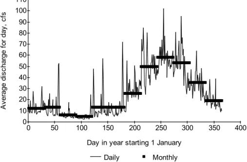
The average of the daily discharges and the monthly discharges are presented in Figure 1. Two observations are illustrated by Figure 1. The first is the large variability of the average daily streamflows even when each day has between 39 and 44 observations and 2) is the damping effect of the average monthly streamflows on the variability. There are a total of 456 months in the data set. Only years with discharges for all twelve months are used. There are data for 38 water years (1952-1980, 1982, 1999, and 2004-2010).
0 10 20 30 40 50 60 70 80 90 100 110 0 50 100 150 200 250 300 350 400 Av er ag e di sc ha rg e fo r da y, c fs
Day in year starting 1 January Daily Monthly
Figure 1. Average daily and monthly streamflows in the Pago River near Ordot, Guam. USGS Station 16865000.
2. The Colwell Index.
The basic concept of the Colwell Index, as applied to monthly streamflows, is that the time periods of the data are calendar months and the state is the monthly discharge which is placed into a class of streamflows. The time (a month) and class define a ‘bin’
containing the number of monthly streamflows in the specific month that are also in the class. Each ‘bin’ has an upper and lower bound of monthly streamflows. The discharge and months form a matrix of rows (discharge classes) and columns (months). Constancy (C) is maximized when all row sums but one are zero (i.e. the variable is constant). Contingency (M) represents the degree time determines state (discharge), or the degree they are dependent on each other.
2.1. Calculation of the Colwell Index
The calculation of the Colwell Index requires a number of decisions. 2.1.1 Decision 1. Select number of time steps.
The literature and logic of the presentation in the Colwell paper indicates the time steps should be the same as the data. If daily data is used the time steps should be days and if
time steps –in that case the data should be by season. In this paper monthly data are used; hence, monthly time steps are used.
2.1.2 Decision 2. Define the class (bin) boundaries.
The bins have boundaries with a uniform difference between the upper and lower boundary of the bins. Sometimes a linear progression is used (B(i) = B(i-1) + C) for the boundary, and sometimes a log progression is used (log(B(i)) = log(B(i-1)) + C). In this paper the log progress is called a log-2 progression because the constant in the log equation has been assumed to be 2. The equations used to determine the bin boundaries in this paper are:
linear bins: B(i) = α C1 Qm α = i from i = 1, 2, ,n-1 log-2 bins: B(i) = 2α C2 Qm α = i-1 from i = 1, 2, ,n-1
where B(i) is the upper bound on class i, Qm is either the median monthly discharge or the mean discharge, n is the number of classes, and C1 and C2 are constants. The last class (i = n) contains the values larger than the upper boundary of the n-1 state.
For the calculation the Colwell Index using monthly streamflow data, the following equations define C1 and C2:
C1 = 4.4/(n-1) C2 = 16.0/(2.0(n-1))
for 12 classes C1 is 0.4 and C2 is 0.015625. The upper bound of the n-1 cell is 4.4 times Qm for arithmetic cell and 16.0 times Qm for log-2 cells. The Guam streamflow data was used in an empirical process using judgment to develop the constants C1 and C2.
There is a third alternative that has been used to calculate the class boundaries. That is the method used in the daily model developed by Henriksen et al (2006). This model calculates the Colwell Index using the following equation for the class boundaries:
B(i) = Qm0.25α α = 0.4, 1, ···, 9
Eleven discharge classes are used in the Henriksen et al model.
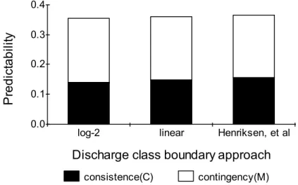
The Cowell Index calculated using the three alternative methods of defining the class boundaries is presented in Figure 2 for the Pago River near Ordot, Guam. There is not much difference. Log-2 progression will be used in this paper.
2.1.3 Decision 3. Select number of discharge classes.
The number of discharge classes can have a significant impact on the values of the Colwell parameters as is illustrated in Figure 3. The reason for the high predictability for the smallest number of discharge classes is that the first class has most of the monthly values. For the Pago River data analyzed with 6 streamflow classes, 51% of the monthly streamflows are in the first class. This contrasts to the situation with 12 discharge classes where 0.6% of the monthly discharge values are in the first class and the highest
percentage. 20% is in the 9th class. Placing a high percentage of the values in the first class makes for a rather constant river.
2.2.4 Decision 4. Select the reference discharge.
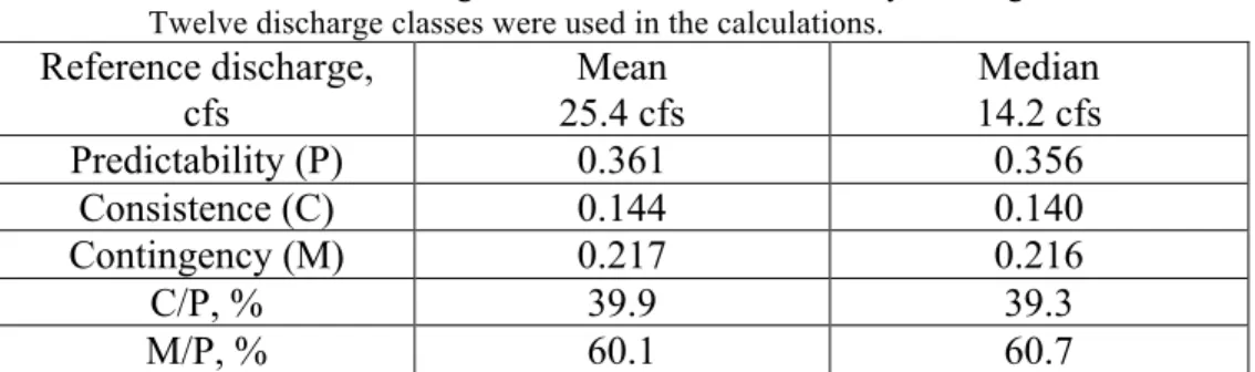
reference discharge could be any discharge – the most common are the mean (average) discharge and the median discharge. The choice of reference discharge does have some impact on consistence as is shown in Table 1. The selection of the reference discharge between median and mean does not have a major impact on the Colwell parameters when 12 discharge classes are used in the analysis. The reference discharge has a significant impact on the Colwell Index when a small number of discharge classes are used.
0.0 0.1 0.2 0.3 0.4
log-2 linear Henriksen, et al
P re d ict a b ili ty
Discharge class boundary approach
consistence(C) contingency(M)
Figure 2. The Colwell Index calculated using three alternative methods of defining class (bin) boundaries for monthly streamflows in the Pago River near Ordot, Guam. There were twelve classes with a reference discharge being the median monthly discharge for the log-2 and linear analysis.
0.0 0.1 0.2 0.3 0.4 0.5 0.6 0.7 6 9 12 15 P re d ict a b ili ty
Number of discharge classes
consistence(C) contingency(M)
Figure 3. The Colwell parameters for the Pago River near Ordot, Guam as related to the number of discharge states used in the analysis. The reference discharge used in the calculation of the discharge states was the median monthly discharge of 14.2 cfs.
2.1.5 Summary of decisions
The Colwell Index model adopted for this paper has the following characteristics: 1. Uses monthly discharge time steps
2. Uses the equation B(i) = 0.015625 (2)α Qm where α = i-1 from i = 1, 2, ,11 for the discharge class boundaries where Qm, is the reference discharge.
3. Uses 12 discharge classes with the 12th class being all monthly discharges larger than the 11th class boundary.
4. Uses the median monthly discharge as the reference discharge.
Table 1. The Colwell parameters for the Pago River near Ordot, Guam (USGS Station 16865000). The reference discharge used in the calculation of the bin sizes was either the mean discharge of 25.4 cfs or the median daily discharge of 14.2 cfs. Twelve discharge classes were used in the calculations.
Reference discharge, cfs Mean 25.4 cfs Median 14.2 cfs Predictability (P) 0.361 0.356 Consistence (C) 0.144 0.140 Contingency (M) 0.217 0.216 C/P, % 39.9 39.3 M/P, % 60.1 60.7
3. Application of the Colwell Index
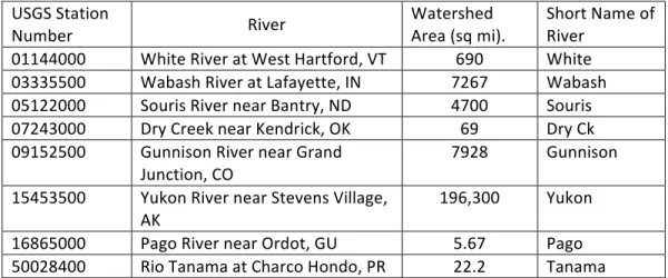
3.1. Variation between riversEight streams were selected to demonstrate variation in the Colwell Index. The watershed areas and USGS station numbers of the eight streams are given in Table 2. The short names in Table 2 will be used on the figures in this section. Results of the Colwell Index calculations are presented in Figure 4. All of the data used to calculate the Colwell Indices were downloaded from the National Water Information System of the US
Geological Survey. The complete record available in December 2011 was used for seven of the eight streams. The exception was the Gunnison River where the record used was up to and including water year 1965.
The eight rivers represent a wide range of watershed types and climates. The White River in Vermont is a vegetated watershed with older geologic materials. The Wabash River watershed is mostly till and is heavily farmed. Both the Souris River and Dry Creek are in the prairies with the Souris in the north and Dry Creek in the south. The Gunnison River starts in the southern Rocky Mountains with lower part in the Colorado Plateau area. The Yukon River is a large northern river. The Pago River has a volcanic watershed on the island of Guam in the middle of the Pacific Ocean. The Rio Tanama, Puerto Rico,
transports water from volcanic material in the upper part and karst terrain in the lower part. Selected statistical parameters for the eight rivers are presented in Table 3. The
skewness shown in the table is the ratio between the mean and the median discharge and is not the same as data skew. Not only do the eight rivers represent a wide range of climate and watershed characteristics but a wide range of discharges (median discharge between 6.2 cfs and 75,510 cfs).
Table 2. USGS station numbers, name and watershed areas for eight American rivers. 0.0 0.1 0.2 0.3 0.4 0.5 0.6 0.7 0.8 0.9
White Wabash Souris Dry Ck Gunnison Yukon Pago Tanama
P re d ict a b ili ty o f st re a m flo w s River consistence contingency
Figure 4. Colwell Index for eight American rivers. The index was calculated using twelve discharge classes defined using the median discharge.
The Cowell Index does allow for a comparison of rivers. Remember, the consistency represents the annual, or seasonal, pattern of flows. As an example, the three rivers with strongest seasonal pattern, contingency, are the Gunnison River (mountain snowmelt), the Yukon River (major spring melting), and the Pago River (wet-dry seasonal pattern). The contingency for the Pago and Gunnison Rivers is essentially the same (0.22) but the reasons for the contingency are rather different.
USGS Station
Number River Watershed Area (sq mi). Short Name of River 01144000 White River at West Hartford, VT 690 White
03335500 Wabash River at Lafayette, IN 7267 Wabash 05122000 Souris River near Bantry, ND 4700 Souris 07243000 Dry Creek near Kendrick, OK 69 Dry Ck 09152500 Gunnison River near Grand
Junction, CO 7928 Gunnison
15453500 Yukon River near Stevens Village,
AK 196,300 Yukon
16865000 Pago River near Ordot, GU 5.67 Pago 50028400 Rio Tanama at Charco Hondo, PR 22.2 Tanama
Table 3. Selected statistical parameters for eight American Rivers. The skewness is the ratio between the mean and the median discharge. The discharge units are cubic feet/second (cfs).
river discharge, median cfs mean discharge, cfs skewness minimum discharge, cfs maximum discharge, cfs number of Years White 814.5 1221.1 1.499 77.5 7286 94 Wabash 4731.5 6866.7 1.451 434.8 42,040 87 Souris 57.35 257.46 4.489 0 11,110 74 Dry Creek 6.18 26.3 4.260 0 308.8 39 Gunnison 1115 2607 2.338 152.8 19,630 57 Yukon 75510 119200 1.579 14800 614,100 35 Pago 14.15 25.42 1.796 0 194.6 38 Rio Tanama 81.8 100.8 1.232 15.8 447.9 30 3.2 Variation caused by water management
Streamflows of the Gunnison River in western Colorado have been measure stating in 1897 and continuing thru the present with 12 incomplete or missing years in the early part of the record. The record may be divided into three periods. The first period is from the beginning of record until construction of a major upstream reservoir completed in 1937 and then thru to construction of Blue Mesa Reservoir which was completed in 1965
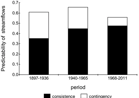
(Milhous 1995). Selected statistical parameters for the three periods are presented in Table 4. The Cowell Index was calculated for each of the periods and presented in Figure 5 with the numbers in Table 5. The consistence increased in all three periods and the contingency decreased.
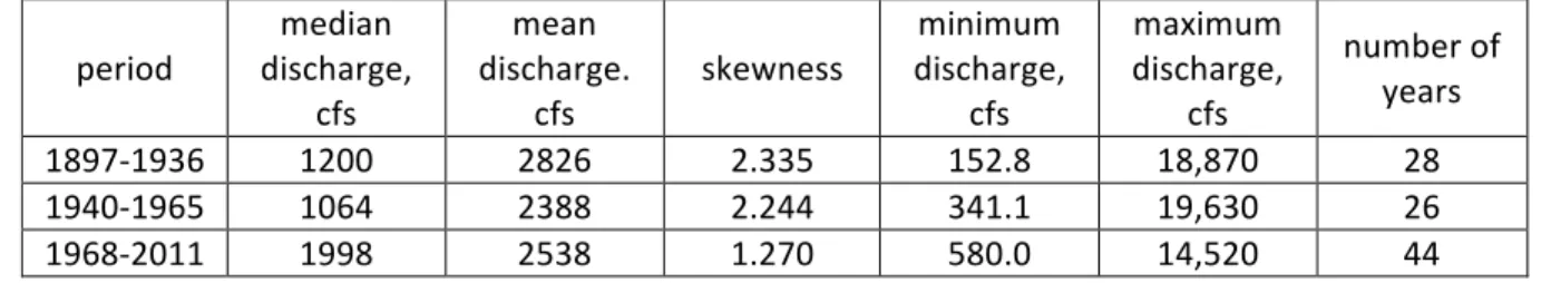
Table 4. Selected statistical parameters for three periods of streamflows in the Gunnison River, Colorado. The skewness is the ratio between the mean and the median discharge. The units for all the discharge are cubic feet/second (cfs).
period discharge, median cfs mean discharge. cfs skewness minimum discharge, cfs maximum discharge, cfs number of years 1897-‐1936 1200 2826 2.335 152.8 18,870 28 1940-‐1965 1064 2388 2.244 341.1 19,630 26 1968-‐2011 1998 2538 1.270 580.0 14,520 44 Thoms and Sheldon, 2000, made an analysis of four rivers in the Barwon–Darling River Basin in Australia comparing simulated natural flows to managed flows. The study showed that water management using nine headwater dams, 15 main channel weirs and 267 diversions resulted in an increase in predictability of streamflows, as represented by the Colwell Index, in all four rivers. The consistency also increased in all four. In two of the rivers the contingency was about the same but in the other two the contingency was slightly reduced. The increase in the consistency also increased in the Gunnison River but the reduction in the contingency was much larger.
4 Discussion and Conclusions
This paper had three principle objectives. The first objective was to present the
Unfortunately, there were many alternative approaches to actually calculating the index. For that reason it is the second and third objectives that are of most interest.
The second objective was to develop consistent method of calculating the Colwell Index for monthly time series of streamflows. That consistent method presented includes 12 discharge states with log-2 scaling of the divisions between the discharge states based on a reference discharge of the median of the monthly streamflows. The series of
boundaries is 0.015625Qm, 0.03125Qm, 0.0625Qm, 0.125Qm, 0.25Qm, 0.5Qm, 1.0Qm, 2.0Qm, 4.0Qm, 8.0Qm, and 16.0Qm where Qm is the median monthly discharge. The 12th discharge state is all monthly discharges larger than 16.0Qm.
The third objective is was to take an empirical look at how the Colwell Index works with a range of rivers both in terms of the size of the river and the climate in which the river is located. A conclusion from this analysis is that the index does show significant difference in the consistency and the annual variation (contingency) of the streamflows. The analysis also showed the impacts on the index of water management in the Gunnison River. 0.0 0.1 0.2 0.3 0.4 0.5 0.6 0.7 1897-1936 1940-1965 1968-2011 P re d ict a b ili ty o f st re a m flo w s period consistence contingency
Figure 5. Colwell Predictability Index for three time periods of streamflow in the Gunnison River in Western Colorado. Index was calculated using twelve discharge states defined using the median discharge.
In this paper no attempt was made to link biology to the Colwell Index. Beissinger (1986) did make a link when the Colwell Index and biology in an application of the index liking Everglades water levels to the reproduction of the Snail Kite (Rostrhamus
Kite demographic traits appear to be adaptations to or results of an uncertain environment. Based on 67 years of Everglades water levels, environmental predictability, measured by spectral analysis and Colwell's (1974) index, was low and influenced by water management regimes: (1) water levels were lowered, (2) annual variation in levels increased and annual cycles became stronger, (3) the period length of long-term drought-flood cycles shifted from 10 or more years toward 5 years, and (4) levels became a less predictive cue for favorable nesting conditions.
The principle value of the Colwell Index is in the making of a comparison of the
uncertainty of the variable stream environments. This ability to use one index to make a comparison of uncertainty may make the Colwell Index a valuable tool in the analysis of environmental flow needs.
A final cautionary note: the Colwell index from different studies should not be
compared unless the same approach to the definition of the limits on the discharge states is used.
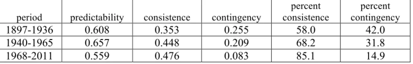
Table 5. Colwell Predictability Index for three time periods of streamflow in the Gunnison River in Western Colorado. The index was calculated using twelve discharge classes defined using the median discharge for the first period (1897-1936).
period predictability consistence contingency
percent consistence percent contingency 1897-1936 0.608 0.353 0.255 58.0 42.0 1940-1965 0.657 0.448 0.209 68.2 31.8 1968-2011 0.559 0.476 0.083 85.1 14.9
References
Beissinger, Steven. 1986. Demography, environmental uncertainty, and the evolution of mate desertion in the Snail Kite. Ecology, Vol. 67, No. 6 (Dec., 1986), pp. 1445-1459.
Colwell, R.K. (1974) Predictability, constancy, and contingency of periodic phenomena. Ecology, 55, 1148-1153.
Fontaine, Richard A. 2003. Flooding Associated with Typhoon Chata’an, July 5, 2002, Guam. Fact Sheet 061-03. U.S. Geological Survey. Honolulu, HI. 96813. 4 pages. Downloaded from
http://hi.water.usgs.gov/ on 15 November 2011.
Gordon, Nancy D., Thomas A. McMahon, Brian L. Finlayson, Christopher J. Gippel, Rory J. Nathan. 2004. Stream Hydrology: An Introduction for Ecologists, Second Edition. John Wiley & Sons, Ltd. Henriksen, J. A., Heasley, J., Kennen, J.G., and Niewsand, S. 2006. Users' manual for the hydroecological
integrity assessment process software (including the New Jersey Assessment Tools). U.S. Geological Survey. Open File Report 2006-1093. 71 p.
Milhous, R.T. 1995. Changes in sediment transport capacity in the lower Gunnison River, Colorado, USA. in Petts, Geoffrey. editor. Man’s Influence on Freshwater Ecosystems and Water Use. IAHS Publication 230. pp 275-280.
Poff, N.L., Ward, J.V. 1989. Implications of streamflow variability and predictability for lotic community structure: a regional analysis of streamflow patterns. Canadian Journal of Fisheries and Aquatic Sciences 46: 1805–1818.
Thoms, M.C., F. Sheldon. 2000. Water resource development and hydrological change in a large dryland river: the Barwon–Darling River, Australia. Journal of Hydrology, 228, 10–21