DISSERTATION
THE ACTIVE COMPLEX ELECTRODE (ACE1) ELECTRICAL IMPEDANCE TOMOGRAPHY SYSTEM & ANATOMICALLY INSPIRED MODELING OF
ELECTRODE-SKIN CONTACT IMPEDANCE
Submitted by Michelle M. Mellenthin
Graduate Degree Program in Bioengineering
In partial fulfillment of the requirements For the Degree of Doctor of Philosophy
Colorado State University Fort Collins, Colorado
Summer 2016
Doctoral Committee:
Advisor: Jennifer L. Mueller Kevin Lear
Diego Krapf Ali Pezeshki
Copyright by Michelle M. Mellenthin 2016 All Rights Reserved
ABSTRACT
THE ACTIVE COMPLEX ELECTRODE (ACE1) ELECTRICAL IMPEDANCE TOMOGRAPHY SYSTEM & ANATOMICALLY INSPIRED MODELING OF
ELECTRODE-SKIN CONTACT IMPEDANCE
Electrical Impedance Tomography (EIT) is a technique used to image the varying elec-trical properties of biological tissues or tissue conductivity and permittivity. There are many clinical uses of EIT, but as a newer imaging modality, there is interest in improving hard-ware to acquire EIT data, creating models of the system and generating high quality images. The two main contributions of this work include: (1) EIT hardware advancements and (2) software modeling to simulate measured human subject data. Specifically, this dissertation includes the design and testing of Colorado State University’s first EIT system, the pairwise current injection active complex electrode (ACE1) system for phasic voltage measurement. The ACE1 system was primarily designed for thoracic EIT applications, and its performance and limitations were tested through a variety of experiments. Additionally, the EIT forward problem was used to investigate electrode-skin contact impedance.
ACKNOWLEDGEMENTS
I am grateful for the many people that have supported me during my academic pursuits. Firstly, I would like to thank my parents, Jim and Mary Mellenthin for supporting me throughout the entirety of my education. I also would like to thank my husband, Christopher Huizenga, for his encouragement.
I thank Jennifer Mueller for her efforts and assistance as my advisor. Not only has she taught me about the field of Electrical Impedance Tomography (EIT), but also about life. Additionally, I’d like to acknowledge the other members of my committee Kevin Lear, Diego Krapf and Ali Pezeshki. A special thanks are extended to my Colorado State University (CSU) colleagues in the EIT lab, especially Melody Alsaker and Rashmi Murphy.
During 2012-2013, the International Institute of Education Whitaker Fellowship Program gave me the opportunity to collaborate internationally. I am extremely grateful to present and former members of the EIT lab at the Universidade de S˜ao Paulo (USP): Raul Gonzalez Lima, Fernando Silva de Moura, Erick Dar´ıo Le´on Bueno de Camargo, Olavo Luppi Silva and Talles Batista Rattis Santos. I sincerely thank them for their advice and assistance. There were many hours spent soldering, testing components, making cables, and the construction of the the ACE1 device would have been very difficult without the efforts of those at CSU and USP.
Much of this doctoral research project was supported by Award Number 1R21EB016869-01 A1 from the National Institute of Biomedical Imaging and Bioengineering. The content is solely my responsibility and does not necessarily represent the official view of the National Institute of Biomedical Imaging and Bioengineering or the National Institutes of Health.
TABLE OF CONTENTS
Abstract . . . ii
Acknowledgements . . . iii
List of Tables . . . ix
List of Figures . . . xii
Chapter 1. Specific Aims and Research Summary . . . 1
1.1. Aim One: The Active Complex Electrode (ACE1) EIT System . . . 1
1.2. Aim Two: Anatomically Inspired Modeling of Electrode-Skin Contact Impedance . . . 3
Chapter 2. An Overview of Electrical Impedance Tomography . . . 4
2.1. Tissue Impedance . . . 4
2.2. EIT for Medical Imaging . . . 7
2.2.1. Types of EIT Images . . . 7
2.2.2. Brain Imaging. . . 8
2.2.3. Breast Cancer Detection . . . 10
2.2.4. Thoracic Imaging . . . 11
2.3. A Brief History of Medical EIT Hardware . . . 13
2.4. A Review of EIT Systems . . . 14
2.4.1. EIT Systems with Planar Arrays . . . 15
2.4.2. EIT Systems for Thoracic Imaging . . . 15
2.4.2.1. Common Current Injection Configurations in Thoracic EIT . . . 16
2.4.2.3. A Review of Existing Academic Thoracic EIT Systems . . . 17
Chapter 3. Analog Hardware Overview: The ACE 1 System. . . 21
3.1. Active Electrodes . . . 25
3.1.1. Active Complex Electrode Design Used in ACE1 . . . 25
3.1.2. Practical Cable Design Considerations . . . 28
3.2. Current Source Design . . . 30
3.2.1. Bipolar Current Source Design . . . 31
3.3. Application of Current through Multiplexers and Logic Circuits . . . 32
3.4. Safety Considerations in ACE1 Design . . . 33
Chapter 4. System Tests Relating to Performance . . . 36
4.1. Estimating Improved Howland Source Output Impedance . . . 36
4.1.1. Ideal Output Impedance . . . 37
4.1.2. Simulated Effects of Op Amp Selection on Source Performance . . . 39
4.2. ACE1 Source Output Impedance . . . 41
4.2.1. Effective Source Output Impedance . . . 42
4.2.2. Mismatch of the Source . . . 47
4.3. System Characteristics . . . 51 4.3.1. Resolution . . . 53 4.3.2. Precision . . . 53 4.3.2.1. Relative Precision . . . 59 4.3.3. Accuracy . . . 61 4.3.3.1. Relative Accuracy . . . 65 4.3.4. Reproducibility . . . 66
4.4. Distinguishability Experiments . . . 78
4.5. Select Reconstructed Images from ACE1 . . . 86
4.5.1. Tank Phantom Images . . . 86
4.5.2. Images of Healthy Human Subjects . . . 86
Chapter 5. System Tests Relating to Noise . . . 89
5.1. Signal-to-Noise Ratio (SNR) . . . 89
5.1.1. Variations in SNR in Comparison to Electrode Position. . . 91
5.1.2. Variations in SNR of Injection Electrodes Compared to Skip Pattern and Acquisition Rate . . . 94
5.1.3. Psuedo-SNR of Human Subject Data . . . 98
5.2. Frequency Components in ACE1 Data . . . 101
5.3. Stray Capacitance Influencing ACE1 . . . 104
5.3.1. Stray Capacitance and Injected Current . . . 104
5.3.2. Stray Capacitance at the Electrode . . . 105
5.3.3. In Between the Source and Node Vc . . . 107
Chapter 6. The Effects of Contact Impedance in EIT . . . 111
6.1. Metal Electrode - Saline Contact Impedance . . . 111
6.1.1. Contact Impedance and ACE1 Tank Phantom Data . . . 113
6.2. Electrode - Skin Contact Impedance . . . 114
6.2.1. Contact Impedance and ACE1 Human Subject Data . . . 115
6.2.2. Determining the Conductivity of the ECG Electrodes. . . 116
6.3. Anatomy of the Human Skin . . . 120
6.5. Modeling Current Penetration Through the Skin . . . 124
Chapter 7. The EIT Forward Problem . . . 131
7.1. The Conductivity Equation . . . 131
7.2. Finite Element Formulation . . . 133
7.3. Electrode Models . . . 135
7.3.1. The Gap Model . . . 135
7.3.1.1. Gap Model Simulations . . . 136
7.3.2. The Shunt Model . . . 136
7.3.3. The Complete Electrode Model (CEM) . . . 137
7.3.3.1. CEM - Skin Interface Simulations . . . 139
7.3.4. The Patacon Model . . . 140
7.4. Implementing an Anatomically Inspired Electrode Model . . . 142
7.4.1. Creation of an Anatomically Representative Mesh . . . 144
7.4.1.1. Set-up in the Finite Element Mesh . . . 145
7.4.2. Comparisons of Different Electrode Models and Human Subject Data . . . 146
7.4.2.1. Implementing the Anatomically Inspired Model . . . 146
Chapter 8. Conclusions . . . 154
8.1. The ACE1 System . . . 154
8.2. The Anatomically Inspired Model . . . 155
References . . . 157
Appendix A. Current Source Design . . . 173
A.2. Improved Howland Design . . . 175
A.3. Bipolar Source from One AC Voltage Input . . . 176
A.4. Increasing Source Output Impedance . . . 177
A.4.1. NIC Design Theory . . . 178
A.4.2. GIC Design Theory . . . 179
Appendix B. Additional System Test Results . . . 182
B.1. Additional Precision Figures & Discussion . . . 182
B.2. Additional Distinguishability Figures . . . 183
Appendix C. Additional Results from Tests Relating to Noise . . . 204
C.1. SNR on a Homogeneous Tank . . . 204
C.2. Additional FFTs of ACE1 Raw Data at Multiple Frequencies . . . 209
Appendix D. Detailed Formulation of 2-D Triangular Finite Elements in EIT . . . 212
D.1. Shape Functions for Triangular Elements . . . 213
D.2. Weak Form Derivation for Local Conductivity Matrix . . . 214
D.3. Example of Assembling Local Matrices . . . 216
Appendix E. Testing of the Forward Problem Code . . . 218
E.1. Comparison of the Forward Problem to Tank Data. . . 218
E.2. Comparison of Anatomical Cross-Section Forward Problem Model to Human Data . . . 219
LIST OF TABLES
2.1 Accepted values for bulk conductivity and permittivity of human tissues at 100 kHz [1–3]. . . 6 2.2 A comparison of key features of commercial thoracic EIT Systems is presented. . . 18 2.3 A comparison of key features of selected academic thoracic EIT Systems is
presented. . . 20
3.1 Frame rates for ACE1 for varying numbers of electrodes and data point acquisition rates. . . 24
4.1 Percent accuracy (%Apk)mean and percent precision (%Ppk)mean of voltage
amplitudes at the 512 and 1024 point acquisition rates as calculated by Equations (4.37) and (4.26) respectively for 0.25 Vpk applied. . . 52
4.2 Percent precision (%Pθ)mean of voltage phase at the 512 and 1024 point acquisition
rates as calculated by Equation (4.30) for 0.25 Vpk applied. . . 52
5.1 A comparison of the average SNR of Ve measurements for injecting electrodes is
presented. 251 frames of data was taken on a tank phantom filled with a saline solution a small ground was placed in the center. Current was injected at 125 kHz. The peak-to-peak voltages correspond to function generator settings of the VCCS. 256, 512, or 1024 indicated the number of samples acquired.. . . 96 5.2 A comparison of the average SNR of Ve measurements for injecting electrodes is
presented. 251 frames of data was taken on a tank phantom filled with a saline solution with no ground in the center. Current was injected at 125 kHz. The
peak-to-peak voltages correspond to function generator settings of the VCCS. 256,
512, or 1024 indicated the number of samples acquired. . . 97
5.3 A comparison of the average SNR of Ve measurements for injecting electrodes for different frequencies for 256 point acquisition rate. . . 99
5.4 A comparison of the average SNR of Ve measurements for injecting electrodes for different frequencies for 512 point acquisition rate. . . 99
6.1 Anatomical and physiologyical properties of human skin [4–7]. . . 122
6.2 Capacitive reactance of a 1 cm2 skin section of human skin [7]. . . 123
6.3 Parameters used in the proposed anatomically inspired skin model.. . . 127
7.1 Values used (which are relevant at approximately 100 kHz) in the anatomical forward problem model for subject 60 [2]. . . 145
7.2 Parameters used in the proposed anatomically inspired skin model.. . . 149
7.3 Percent error of the different electrode models with one standard deviation. . . 150
C.1 A comparison of the average SNR of Ve measurements for injecting electrodes is presented. 251 frames of data was taken on a tank phantom filled with a saline solution with no ground in the center. Current was injected at 75 kHz. The peak-to-peak voltages correspond to function generator settings of the VCCS. 256, 512, or 1024 indicate the number of samples acquired. . . 206 C.2 A comparison of the average SNR of Ve measurements for injecting electrodes is
presented. 251 frames of data was taken on a tank phantom filled with a saline solution with no ground in the center. Current was injected at 100 kHz. The
peak-to-peak voltages correspond to function generator settings of the VCCS. 256, 512, or 1024 indicate the number of samples acquired. . . 207
LIST OF FIGURES
3.1 The basic design and acquisition of data with the active complex electrode (ACE1) system is described with this block diagram. . . 21 3.2 The ACE1 tomograph cables connected to a human volunteer (left) and a photo
of the portable system (right). . . 22 3.3 This figure illustrates the pairwise injection of current about the domain for a skip
four pattern. The direction of bipolar current flow is indicated by the arrows. . . 23 3.4 This diagram illustrates the basic active electrode implementation design. An
operational amplifier used in the follower configuration is simplest of active
electrode designs. . . 25 3.5 Figure A depicts a simplified schematic of the active electrode design. Figure B
shows raw data from an injecting electrode pair. During each current pattern, the first samples acquired are of voltages at the electrode (Ve). Using switches allows
for acquisition of Vc. Current is determined from Vc, Ve, and Rsense. . . 26
3.6 The ACE1 electrode iterations became progressively more robust to mechanical forces experienced in certain clinical applications through thicker wire and stronger wire mount connections to the board. . . 29 3.7 The differences between a monopolar current source and a bipolar current source
can be seen in this figure. In (a), a Skip 1 pattern is used to inject current into the domain. In (b), a Skip 1 pattern with the bipolar source is shown. For the bipolar, I− and I+ are 180 degrees out of phase with one another. . . 31
3.9 The interaction of digital signals from the parallel port, logic circuits and multiplexer to control pairwise current injection and measurement of different
nodes in the active electrode is shown. . . 33 3.10 ACE1 cables in an anti-static encasing for ease of cleaning and reducing short
circuit risks. . . 35
4.1 Improved Howland circuit model [8], where Vt− = Vt+ = Vt when assuming ideal
op amp behavior. . . 37 4.2 Multisim circuit showing the test configuration for Zout. Inputs are grounded
to the source and a voltage source is placed at the output. C3 and C41 are
DC-blocking capacitors that were added to the improved Howland design to block any DC offsets. . . 40 4.3 Multisim was used to test several different op amps to see which yielded the
highest output impedance for frequencies larger than 100 kHz. The test setup from Figure 4.2 was used. R designates the resistor values for R11, R12, R13, R14,
and r is R15. C is the value of the DC blocking capacitors. . . 41
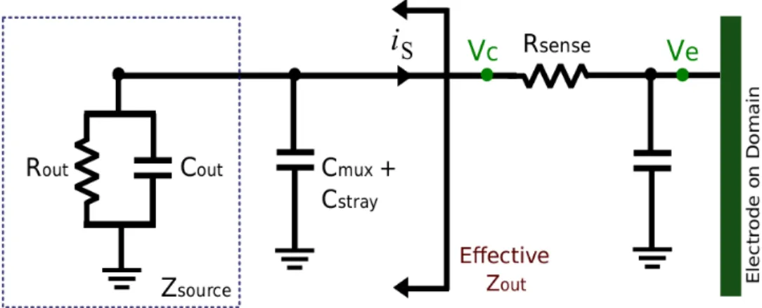
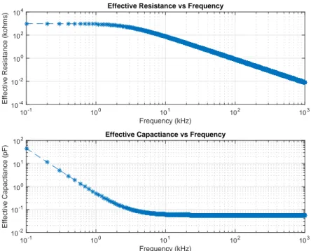
4.4 The output impedance of the ACE1 current source from isolated testing. . . 42 4.5 The effective output resistance of the ACE1 current source, where Rout, Cout and
Cmux+stray describe Zout. . . 43
4.6 The effective output impedance of the ACE1 current source for each current
pattern at 75 kHz (top) and 125 kHz (bottom). . . 44 4.7 The current source output impedance (Zout) as modeled by a resistor (Rout) and
4.8 The effective output impedance of the ACE1 current source. . . 47 4.9 Calculated current amplitude for both parts of the bipolar source as well as their
sum (or mismatch) is plotted for each of the 500 frames (or about 20 seconds) data collected on a healthy human subject during breath holding at 15.8 frames/second with a skip 4 current pattern. 31 electrodes were used. . . 48 4.10 An image of the plastic tank phantom, which has an inner diameter of 30 cm and
contains 32 square stainless steel electrodes (2.54 cm by 2.54 cm) placed 4 mm apart. When 1 liter of saline solution is added, the tank fills to a height of 1.4 cm. 49 4.11 Source mismatch from 30 frames of data taken on a homogeneous tank for different
skip patterns and varying injected currents. . . 50 4.12 Test set-up where all of the ACE1 cables were connected to the same voltage
source and 100 frames of data was collected. Inputs to the ACE1 current source were grounded. . . 51 4.13 The precision (Ppkkl) of measured voltage amplitudes in µV for each electrode for a
single current pattern (k = 18) for a 0.25 Vpk applied voltage at various frequencies
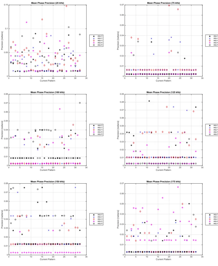
for 100 frames of data acquired at the 1024 point acquisition rate. . . 55 4.14 Mean phase precision in radians for each current pattern ((Pθk)mean) for measured
voltage phases corresponding to a 0.25 Vpk applied voltage at various frequencies
for 100 frames of data acquired at the 1024 point acquisition rate. . . 57 4.15 Overall mean precision for amplitude (Ppk)mean (top row) and phase (Pθ)mean
(bottom row) for different skip patterns and frequencies taken at the 512 acqusition rate (left) and 1024 acquisition rate (right). . . 58
4.16 Overall percent mean precision for amplitude %(Ppk)mean (top row) and phase
Percent %(Pθ)mean (bottom row) for different skip patterns and frequencies taken
at the 512 acqusition rate (left) and 1024 acquisition rate (right). . . 61 4.17 Accuracy and precision of voltage amplitude measurements for a representative
current pattern (k = 18) for a dataset taken at the 512 acquisition rate for a 0.25 Vpeak applied voltage. . . 63
4.18 Accuracy and precision of voltage amplitude measurements for a representative current pattern (k = 18) for a dataset taken at the 1024 acquisition rate for a 0.25 Vpeak applied voltage. . . 64
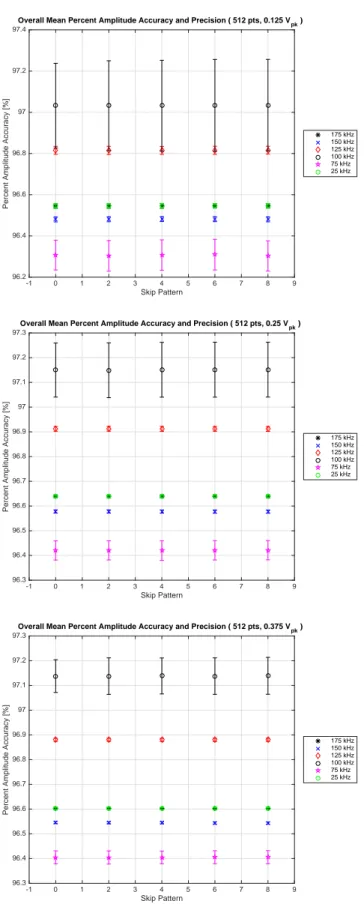
4.19 Overall mean percent amplitude accuracy and precision for the 512 point acquisition from 100 frames of data measuring a 0.125 Vpk, 0.25 Vpk and 0.375 Vpk
applied voltage. . . 67 4.20 Overall mean percent amplitude accuracy and precision for the 512 point (left)
and 1024 point acquisition rate (right) from 100 frames of data measuring a 0.25 Vpk applied voltage. . . 68
4.21 Reproducibility of homogeneous tank data voltage amplitude measurements at different frame rates is shown for 75 kHz (left) and 125 kHz (right). Data was also taken at a different acquisition rates: 256 points (row 1), 512 points (row 2) and 1024 points (row 3). . . 69 4.22 Overall mean amplitude reproducibility (top row) and overall mean percent
amplitude reproducibility (bottom row) of different skip patterns for 75 kHz (left) and 125 kHz (right) for the 256 point, 512 point and 1024 point acquisition rates. 70
4.23 Reproducibility of homogeneous tank data voltage phase measurements is shown for 75 kHz (left) and 125 kHz (right). Data was also taken at a different acquisition rates: 256 points (row 1), 512 points (row 2) and 1024 points (row 3). . . 73 4.24 Percent phase reproducibility for homogeneous tank data taken at the at the 1024
point acquisition rate is shown for 75 kHz (left) and 125 kHz (right) for three
different current patterns: 7 (row 1), 13 (row 2), 25 (row 3). . . 74 4.25 Phase reproducibility is radians at 75 kHz is shown for the different acquisition
rates for skip patterns: 0, 2, 4, 6, and 8. . . 75 4.26 Phase reproducibility is radians at 125 kHz is shown for the different acquisition
rates for skip patterns: 0, 2, 4, 6, and 8. . . 76 4.27 Overall mean phase reproducibility (top row) and overall mean percent phase
reproducibility (bottom row) of different skip patterns for 75 kHz (left) and 125 kHz (right) for the 256 point, 512 point and 1024 point acquisition rates. . . 77 4.28 Distinguishability experiment targets are made from 1/4 in, 3/8 in, 1/2 in, and
3/4 in plastic and copper pipe. The corresponding outer diameters for the plastic targets (P1, P2, P3, P4) are: 0.95 cm, 1.3 cm, 2.2 cm, and 2.88 cm. Outer diameters for the copper targets (C1, C2, C3, C4) are: 1.1 cm, 1.45 cm, 1.8 cm and 2.45 cm. . . 78 4.29 Distinguishability plots for all targets and skip patterns for frequencies (25 kHz to
100 kHz) where the overall mean calculation uses mean measured voltage over all electrodes and current patterns. . . 81
4.30 Distinguishability plots for all targets and skip patterns for frequencies (125 kHz to 175 kHz) where the overall mean calculation uses mean measured voltage over all electrodes and current patterns.. . . 82 4.31 Mean distinguishability plots for data collected at 125 kHz for current pattern (k)
number 10 for various skip patterns 0, 2, 4, 6, and 8 (which are the best for 32 electrodes by Equation 3.1 where C1, C2, C3 and C4 are the copper pipe tank phantom targets. . . 84 4.32 Mean distinguishability plots for data collected at 125 kHz for current pattern (k)
number 10 for various skip patterns 0, 2, 4, 6, and 8 (which are the best for 32 electrodes by Equation 3.1 where P1, P2, P3 and P4 are the plastic pipe tank phantom targets. . . 85 4.33 Picture A shows the experimental setup of the tank filled with saline and three
cucumber phantoms. Reconstructions by Jennifer Mueller show conductivity (B) and permittivity (C). . . 86 4.34 Shown are reconstructed conductivity images of the cardiac cycle in a healthy
human subject by Melody Alsaker. The six sequential images show the heart moving from systole (contraction) to diastole (relaxation and filling) at 15.8
frames/sec. . . 87 4.35 Shown are reconstructed conductivity images of tidal breathing in a healthy
human subject by Melody Alsaker. The six frames show inflation from the lungs from expiration to inspiration to expiration at a frame rate of 15.8 frames/sec. . . . 88
5.1 Single current pattern SNR over 250 frames at the 512 point acquisition rate for a 6 Vpp input and odd skip patterns are shown in the left column and even on the
right. (Row 1) 25 kHz. (Row 2) 50 kHz. . . 92 5.2 Single current pattern SNR over 250 frames at the 512 point acquisition rate for a
6 Vpp input and odd skip patterns are shown in the left column and even on the
right. (Row 1) 75 kHz. (Row 2) 100 kHz. (Row 3) 125 kHz.. . . 93 5.3 Single current pattern SNR over 250 frames at the 512 point acquisition rate for a
6 Vpp input and odd skip patterns are shown in the left column and even on the
right. (Row 1) 150kHz. (Row 2) 175 kHz. . . 94 5.4 SNR on a homogeneous tank phantom data (with a small ground in the center) at
125 kHz for the injection electrodes for different voltage inputs to the VCCS, skip patterns and acquisition rates. . . 95 5.5 Four different human subjects were asked to hold their breath for approximately
20 seconds (or 500 frames). Data was collected at 1024 point acquisition rate with a skip 0 configuration. . . 100 5.6 Average SNR of injection electrodes of several human subjects during breath
holding. . . 101 5.7 FFTs for current pattern 1 and skip 0 for data on different channels of homogeneous
tank when the VCCS input is turned off (top) and when the VCCS input is set to 4.0 Vpp at 100 kHz. . . 103
5.8 This schematic represents the loss of current in between the voltage controlled current source (VCCS) and the load. . . 104
5.9 Circuit model and testing set-up using a precise 1.0 kΩ resistor to determine the
effects of stray capacitance at the electrode. . . 106
5.10 Cstray capacitance with standard deviation for each electrode for 96 current patterns of data. This includes the capacitance from the switch.. . . 107
5.11 Experiment to determine stray capacitance in between the multiplexer (mux) and active electrode, where the combined impedance of the stray and mux capacitance and line and mux resistance is considered Zcable.. . . 108
5.12 The stray capacitance affecting each channel during injection. . . 110
6.1 Saline was added to fill the test cell to a height of 1.72 cm. . . 112
6.2 Mean distinguishability for skip 2 data collected at 125 kHz for current pattern 10 where C1, C2, C3 and C4 are the copper pipe targets (left) and P1, P2, P3 and P4 are the plastic pipe targets (right). . . 113
6.3 Ventilation signals from electrode one on a healthy human subject feeling cool, normal and warm, where the top set of plots is for data taken with skip 0 pattern and the bottom is skip 2. . . 117
6.4 Experimental set-up to determine conductivity of ECG electrode gel. . . 118
6.5 Gel absorbence of sweat based on anatomical location. . . 119
6.6 The anatomy of the human skin [9].. . . 120
6.7 The anatomically inspired skin model, modified from the model proposed by Chizmadzhev [10] for use in EIT. . . 125
6.8 Voltages calculated using parameters for the gel-filled pore model are given for a single pore (top row) from Equation (6.15) and the whole electrode (bottom row) from Equation (6.17). . . 129 6.9 Voltages calculated using parameters for the sweaty pore model are given for a
single pore (top row) from Equation (6.15) and the whole electrode (bottom row) from Equation (6.17). . . 130
7.1 A plot nodal potentials for injecting nodes for the mesh with electrode element conductivities of 0.25 mS/cm (left) and the mesh where currents are imposed
directly long the skin (right). . . 137 7.2 Examples of shunt model current densities.. . . 138 7.3 The finite element mesh with a single CEM electrode made of 64 elements on a
layer of skin and fat. . . 139 7.4 Nodal voltage potentials for electrode parameter of 3.84 mS/cm and varying skin
conducitivites, from left to right: (Row 1) 0.0012 mS/cm, x 0.0018 mS/cm, (Row 2) 0.0024 mS/cm, 0.0036 mS/cm, (Row 3) 0.006 mS/cm and 0.0096 mS/cm. The electrode is located on the boundary from 3.9 to 6.1 cm on the x-axis. . . 141 7.5 Spacing of pores (left) corresponding to an ECG electrode with size 2.2 cm by 3.3
cm (right).. . . 143 7.6 An image of the healthy human subject volunteer (left) and the cross-section of
electrode placement obtained with use of flexible rulers (right). . . 145 7.7 The mesh (top) used for both the antomically inspired model and gap model. The
7.8 Incorporating 32 Hua elements onto the same mesh shown in Figure 7.7. . . 148 7.9 Real voltages on electrodes for measured data, the gap model, the CEM (ρ′
= 3.48) and the anatomically inspired model which uses a uniform current density, σr = 0.525 mS/cm and Cw = 0.075 µF/cm (row 1). Row 2 shows voltages near
the lagging injection electrode (7) and row 3 shows voltages on leading injection electrode (8). . . 151 7.10 Comparison of error for different current patterns (5, 9, and 16) for the gap model,
the CEM (ρ′
= 3.48) and the anatomically inspired model (σr = 0.525 mS/cm and
Cw = 0.075 µF/cm). . . 152
7.11 Comparison of error on injecting electrodes for the CEM and anatomically inspired model (σr = 0.525 mS/cm and Cw = 0.075 µF/cm) for each half of the bipolar,
denoted by +/-. . . 153
A.1 The schematics of the two different Howland designs. . . 173 A.2 The schematic diagram of the bipolar current source shows the incorporation of
two improved Howland designs with an AD8132 differential amplifier. . . 176 A.3 Implementation of a basic NIC design [11]. . . 178 A.4 Implementation of the NIC design proposed by Cook [12]. . . 179 A.5 Implementation of a basic GIC design [13]. . . 180
B.1 The precision (Ppkkl) or one standard deviation for measured voltage amplitudes of
a 0.125 Vpk applied voltage at various frequencies for 100 frames of data acquired
B.2 The precision (Ppkkl) or one standard deviation for measured voltage amplitudes of
a 0.25 Vpk applied voltage at various frequencies for 100 frames of data acquired at
the 512 point acquisition rate. . . 186 B.3 The precision (Ppkkl) or one standard deviation for measured voltage amplitudes of
a 0.375 Vpk applied voltage at various frequencies for 100 frames of data acquired
at the 512 point acquisition rate. . . 187 B.4 Mean phase precision for each current pattern ((Pθk)mean) for measured voltage
phases corresponding to a 0.125 Vpk applied voltage at various frequencies for 100
frames of data acquired at the 512 point acquisition rate. . . 188 B.5 Mean phase precision for each current pattern ((Pθk)mean) for measured voltage
phases corresponding to a 0.25 Vpk applied voltage at various frequencies for 100
frames of data acquired at the 512 point acquisition rate. . . 189 B.6 Mean phase precision for each current pattern ((Pθk)mean) for measured voltage
phases corresponding to a 0.375 Vpk applied voltage at various frequencies for 100
frames of data acquired at the 512 point acquisition rate. . . 190 B.7 Overall mean precision for amplitude (Ppk)mean (left) and phase (Pθ)mean (right)
for different skip patterns and frequencies taken at the 512 point acqusition rate for: 0.125 Vpk (row 1), 0.25 Vpk (row 2) and 0.375 Vpk (row 3). . . 191
B.8 Overall percent mean precision for amplitude Percent (Ppk)mean (left) and phase
Percent (Pθ)mean (right) for different skip patterns and frequencies taken at the
512 point acqusition rate for: 0.125 Vpk (row 1), 0.25 Vpk (row 2) and 0.375 Vpk
B.9 The precision (Ppkkl) or one standard deviation for measured voltage amplitudes of
a 0.375 Vpk applied voltage at various frequencies for 100 frames of data acquired
at the 1024 point acquisition rate. . . 193 B.10 Mean phase precision for each current pattern ((Pθk)mean) for measured voltage
phases corresponding to a 0.375 Vpk applied voltage at various frequencies for 100
frames of data acquired at the 1024 point acquisition rate. . . 194 B.11 Overall mean precision for amplitude (Ppk)mean (left) and phase (Pθ)mean (right)
for different skip patterns and frequencies taken at the 1024 point acqusition rate for: 0.25 Vpk (row 1) and 0.375 Vpk (row 2). . . 195
B.12 Mean distinguishability plots at 25 kHz for current pattern 10 and skip patterns 0, 2, 4, 6, and 8 where C1, C2, C3 and C4 are the copper pipe targets. . . 196 B.13 Mean distinguishability plots at 25 kHz for current pattern 10 and skip patterns
0, 2, 4, 6, and 8 where P1, P2, P3 and P4 are the plastic pipe targets. . . 197 B.14 Mean distinguishability plots at 75 kHz for current pattern 10 and skip patterns
0, 2, 4, 6, and 8 where C1, C2, C3 and C4 are the copper pipe targets. . . 198 B.15 Mean distinguishability plots at 75 kHz for current pattern 10 and skip patterns
0, 2, 4, 6, and 8 where P1, P2, P3 and P4 are the plastic pipe targets. . . 199 B.16 Mean distinguishability plots at 100 kHz for current pattern 10 and skip patterns
0, 2, 4, 6, and 8 where C1, C2, C3 and C4 are the copper pipe targets. . . 200 B.17 Mean distinguishability plots at 100 kHz for current pattern 10 and skip patterns
B.18 Mean distinguishability plots at 175 kHz for current pattern 10 and skip patterns 0, 2, 4, 6, and 8 where C1, C2, C3 and C4 are the copper pipe targets. . . 202 B.19 Mean distinguishability plots at 175 kHz for current pattern 10 and skip patterns
0, 2, 4, 6, and 8 where P1, P2, P3 and P4 are the plastic pipe targets. . . 203
C.1 Single current pattern SNR for 250 frames at the 256 point acquisition rate for 6 Vpp input voltage to the VCCS. (Row 1) 25 kHz, 50 kHz. (Row 2) 75 kHz, 100
kHz. (Row 3) 125 kHz, 150 kHz. . . 205 C.2 Single current pattern SNR for 250 frames at 125 kHz where the voltage input to
the VCCS is set to 4 Vpp (Row 1), 6 Vpp (Row 2), 8 Vpp (Row 3) for the 1024 point
acquisition rate. . . 208 C.3 FFTs of channel measurements for a skip 0 and 2 datasets taken on a human
subject. . . 209 C.4 Raw data measurements and corresponding FFTs of individual channels for a skip
0 dataset at 16.0 frames/second and 125 kHz taken on a human subject. . . 210 C.5 Raw data measurements and corresponding FFTs of individual channels for a skip
2 dataset at 16.0 frames/second and 125 kHz taken on a human subject. . . 211
D.1 A typical triangular element used in the forward problem where the x and y
coordinates define locations of the nodes. . . 212 D.2 An example of a simple three element mesh. . . 216
E.1 A 32 triangle element Hua model corresponding to the placement of the ACE1 tank phantom’s 32 electrodes. . . 218
E.2 Comparing voltages all all electrodes during a single current pattern for simulated and measured data. . . 219 E.3 A 32 element Hua model representing electrodes is consistent with placement
marked in Figure 7.6. . . 220 E.4 Comparisons to skip 0 measured data using parameters in Table 7.1. The
simulation used values for inspired lung since measured data trace corresponds an average for 301 frames of breath holding at 24.9 frames/sec. . . 221 E.5 Comparisons to skip 3 measured data using parameters in Table 7.1. The
simulation used values for lung that were an average of inspiration and expiration because the measured data trace corresponds to 301 frames of tidal breathing at 16.0 frames/second . . . 221
CHAPTER 1
SPECIFIC AIMS AND RESEARCH SUMMARY
This short chapter addresses the context of this work within the Electrical Impedance Tomography (EIT) field. This dissertation aims to increase understanding in the complexities of constructing a new electrical impedance tomograph, addressed through aim one (Section 1.1). It also looks at the electrode-skin contact impedance, specifically how it relates to ACE1 measured data through aim two (Section 1.2).
1.1. Aim One: The Active Complex Electrode (ACE1) EIT System In EIT, the resolution and accuracy of conductivity and/or permittivity images are lim-ited by both hardware and software. The clarity of anatomical features within an image is greatly dependent on the precision of the acquired voltage data. Errors and noise in voltage measurements result in errors of conductivity or permittivity values in the reconstructions. To create images of permittivity, accurate phase information must be known about both the injected currents and measured voltages of an EIT system. The first aim of this work was to design an electrical impedance tomography system in which magnitude and phase of measured voltages and currents can be determined.
An overview of the design of the ACE1 system, which meets the first objective is presented in Chapter 3. An advantage of this system when compared to existing systems, discussed in Section 2.4, is the design of the active electrode, which provides a way to determine the magnitude and phase of injected current close to the domain. The performance of this system is rigorously addressed in Chapter 4. Results related to testing the ACE1 current source are presented in Section 4.2. The output impedance of the source is often used to determine source performance, but measuring the current on the active electrode allows for
use of a source with less than ideal behavior. Output impedance of the source varies based on frequency and tests are consistent with National Instruments Multisim circuit simulations. The overall frame-to-frame variation of calculated currents at the active electrode is low. During human subject data collection, bipolar currents are injected approximately 0.31% ± 0.02% out of phase with one another and with a 1.31% ± 0.09% difference in amplitude.
Chapter 4 also contains results for experiments addressing the resolution, precision, ac-curacy, and reproducibility of data in Section 4.3. ACE1 is able to precisely measure voltage amplitudes to within 27 µV and voltage phase to within 0.045 radians. For tank phantom data, the voltage amplitude measurements are reproducible from frame-to-frame to 60 µV or less and voltage phase measurements to within 0.05 to 0.1 radians. The sensitivity of the system or its ability to distinguish differences in tank phantom targets is presented in Sec-tion 4.4. The difference between a 0.95 cm and 1.3 cm insulator placed in the center of the tank phantom was distinguishable at skips 2, 4 and 6 by several non-injecting electrodes by voltage differences greater than the reproducibility of measured data. Select reconstructed images are also shown in Section 4.5.
Chapter 5 presents results from signal-to-noise ratio (SNR) experiments in Section 5.1. The SNR is highest on injecting electrodes and decays as distance from injection electrodes increases. A mean SNR over all electrodes, current patterns and frames is generally highest for skip patterns 4 to 8 and when data is acquired at the 1024 point acquisition rate. Sec-tion 5.3 aims to estimate stray capacitance at different locaSec-tions within in the EIT system. Results suggest that at 125 kHz, as much as approximately 5% of current is drained by stray capacitance present at the electrode.
1.2. Aim Two: Anatomically Inspired Modeling of Electrode-Skin Contact Impedance
Incorporation of electrode models into reconstruction algorithms is an important part of EIT. This work investigates the role of the forward problem and limitations in modeling the electrode-skin contact impedance. Accurate forward problem simulations must include a model for this contact impedance. When it is not considered, simulated and measured voltages will not agree. The second aim of this dissertation was to use the EIT forward problem to investigate physiologically inspired models of the skin-electrode interface.
To better consider the influence of contact impedance on measured data, both electrode-saline (Section 6.1) and electrode-skin (Section 6.2) contact impedance were investigated. Chapter 6 also presents physiological and anatomical information about skin to give context and motivation for using a model describing current flow through pores of the skin [10] in Section 6.5. This model is modified to be appropriate for use in the EIT forward problem modeling the electrode-skin interface in Section 7.4.
In Chapter 7, the EIT forward problem and electrodes models are discussed in detail. The results of the anatomically-inspired model simulations are compared to existing EIT electrode models and to measured human subject data from the ACE1 system in Section 7.4.2. In some situations, use of this model can help create simulated data that is accurate on both injecting and neighboring electrodes.
CHAPTER 2
AN OVERVIEW OF ELECTRICAL IMPEDANCE TOMOGRAPHY Electrical Impedance Tomography (EIT) is an imaging modality which creates low spa-tial resolution images that map electrical properties. In medical EIT acquisition, small sinu-soidal currents injected on electrodes are passed through a region of the body, and measured voltages are used to solve an inverse problem to recover conductivity and/or permittivity distributions. Due to the electric properties of biological tissues, further discussed in Section 2.1, EIT is a suitable imaging technique for many medical applications [1, 2, 14, 15].
There are several advantages to using EIT as a medical imaging technique. It is radiation-free, non-invasive, low-cost, portable, has a high temporal resolution and could be used for long-term bedside monitoring of patients in many clinical settings. Specific examples of EIT use are further discussed in Section 2.2. Despite its many advantages, EIT has several limitations. It often suffers from low signal-to-noise ratios (SNR) and is sensitive to modeling errors, such as accurate contact impedance and knowledge of electrode placement [14, 15, 2, 16, 11]. The amount of significant clinical information present in EIT images depends greatly upon both the reconstruction algorithm and hardware. In particular, the spatial resolution of reconstructed images of all EIT systems vary because they depend on accuracy and SNR of measured data as well as the algorithm used. System tests for the ACE1, including SNR, are presented in Chapters 4 to 5 .
2.1. Tissue Impedance
In EIT, images are reconstructed to show distributions of conductivity and/or permit-tivity. Conductivity (σ), the inverse of the resistivity, can be defined as the extent to which
electricity flows in a domain or as the charge concentration. A larger conductivity corre-sponds to increased ease of charge movement. Permittivity (ϵ), related to capacitance, is a material’s resistance to forming an electric field [17]. A greater permittivity in a substance corresponds to an increased ability to store electric charge. Conductivity and permittivity are combined in Equation (2.1) to obtain admittivity (γ), where ω = 2πf is the angular frequency in radians/second.
γ = σ + iωϵ (2.1)
Table 2.1 illustrates the differences in bulk conductivity properties of human tissue. A large range in impedance exists within the body. For example, cerebrospinal fluid is 250 times more conductive than bone [1, 2]. In addition, conductivity and permittivity values change based on the physiological states of organs or tissues and with the orientation of the measurement to existing fibers. The electrical characteristics of muscles vary whether they are measured along the fibers (longitudinally) or across the fibers (transversely). Table 2.1 also shows a decrease in lung conductance and permittivity during inspiration [1, 2]. This change in conductivity and permittivity is created by the increase or decrease of air in the lungs, where the resistance of air is greater than tissue.
Bulk electrical properties are helpful in identifying uses of medical EIT and understanding reconstructed EIT images. The higher conductivity of blood and the change in impedance during respiration support use of EIT images for depicting areas of ventilation and perfusion. Presently, conductivity images are the most widely used. However, conductivity images alone are not necessarily sufficient in a clinical setting. EIT images would benefit from the inclusion
Table 2.1. Accepted values for bulk conductivity and permittivity of human tissues at 100 kHz [1–3].
Tissue Conductivity [mS/cm] Permittivity [µF /m]
Cerebrospinal fluid 15.4 —
Blood 6.7 0.05
Liver 2.8 0.49
Skeletal muscle 8.0 long. & 0.6 trans. —
Cardiac muscle 6.3 long. & 2.3 trans. 0.88 long. & 0.36 trans.
Neural tissue 1.7 —
Gray matter 3.5 —
White matter 1.5 —
Lung 1.0 exhale & 0.4 inhale 0.44 exhale & 0.22 inhale
Fat 0.36 0.18
Bone 0.06 0.0027
Skin 0.0012 0.0144
of permittivity, which may make it easier to visualize differences between tissues that have similar resistivities or healthy tissue from anomalies [2, 15].
The frequency chosen for current injection in EIT data acquisition influences which fea-tures within a tissue are emphasized. A lower frequency of injected current is believed to weave around cells in the extracellular matrix, and a higher frequency passes more directly through cells. For example, changes in cellular swelling may be more readily seen with fre-quencies at approximately 200 Hz [11]. Many EIT systems use a mid-range frequency (30 kHz - 200 kHz) in which information relevant to both low and higher frequencies can be obtained [12, 18].
Since electrodes are used in EIT, the high contact impedance between the epidermis of the skin and the electrode results in large electric potential drops at the interface which can mask changes within. Contact impedance is further discussed in Chapter 6. A reason some EIT groups use frequencies of approximately 100 kHz or greater is that higher frequencies can lessen the effects of contact impedance caused by the capacitance associated with the
skin. The skin’s high impedance often creates artifacts along the boundaries of reconstructed images, and improving how it is modeled is one of the challenges in EIT.
2.2. EIT for Medical Imaging
With proper electrode placement, EIT is commonly used to image impedance changes in the brain, breasts, and the chest or thorax to target the lungs and heart [2, 11]. Medical applications of EIT not discussed in detail in this text include use for prostate cancer detec-tion [19, 20] and cervical cancer detecdetec-tion [21, 22]. Developments have led to the creadetec-tion of commercial systems by Zilico [23] and Impedance Medical Technologies [24], which are marketed for cervical screening. EIT has also been considered as a method for monitoring radio-frequency induced hyperthermia, which is a technique used for ablating tumors [11, 25]. Motivation and promising work in EIT for neural imaging, breast cancer detection and thoracic imaging are discussed in subsequent subsections and associated tomographs are discussed in Section 2.4.
2.2.1. Types of EIT Images. EIT images can be either 2-D or 3-D depending on placement of electrodes and reconstruction algorithms used. Images can show structure as well as function. In the creation of EIT difference images, a reference image is chosen and reconstructed images reflect a change in impedance characteristics from the reference. Most EIT data is dynamic or collected over a period of time so that a series of images or a movie can be created. Time-difference dynamic EIT images are particularly useful to image bodily functions or organs and fluids that move within the body, such as blood flow, air flow or stomach s(gastric) emptying. Difference images are commonly created by commercial and research groups because noise from experimental conditions and noise from the electronics or equipment is mostly subtracted out [15, 26]. Sampling and frame rates can be used to
vary the time resolution of images, but there is a direct relationship with the signal-to-noise ratio (SNR) that is discussed in Chapter 5.
There is another type of EIT images that can be obtained. Absolute images do not use a reference frame to create images, but often use a model as a reference during image reconstruction. These types of images are difficult to obtain because the noise from the experimental conditions and equipment is not subtracted out, so it either has to be greatly minimized and/or accurately modeled. Obtaining absolute conductivity EIT images is easier to do than absolute permittivity EIT images. Since permittivity information is taken from voltage phase measurements, small errors introduced by parasitic capacitance can make absolute permittivity EIT images very difficult to obtain. Absolute EIT images are the best for imaging anatomy or structure within the body. Absolute images can be time varying or dynamic or may be a single static image. If a sequence of absolute images is created, functional information can be obtained as well.
2.2.2. Brain Imaging. For approximately 7-8% of patients that experience habitual seizures, surgical intervention to destroy neuronal tissue causing these episodes is a necessary treatment [27]. To have the best surgical outcomes, it is essential to identify the area of the brain that is the greatest contributor for causing seizures and destroy only that tissue. While EIT may someday be routinely used to look for impedance changes in the brain caused by the seizures, other imaging techniques and monitoring methods are presently used. Electroencephalograms (EEGs) are often used to test for basic epileptic characteristics in the brain and magnetic resonance imaging (MRI) and positron emission tomography (PET) are often used to localize cortical abnormalities [28].
Researchers have been exploring EIT as a method for imaging brain function since the early 1990s. Brain activity during an artificially induced stroke was first studied in 1992 by Holder [29]. During a stroke, impedance changes caused by cell swelling and changes in the volume of blood can be detected with EIT. Additionally, Holder and coworkers investigated the use of EIT for imaging fast impedance changes in the brain associated with neuronal activity. EIT has also been used to look at depression [30], localize epileptic foci and measure brain activity during seizures [11, 31, 27, 32]. One of the most promising EIT research studies involving localization of epileptic foci was performed on anaesthetized rabbits in 1996 [32]. In this study, 16 electrodes were placed around perimeter of one plane of the exposed superior surface of the brains of rabbits. Reproducible impedance changes were detected in corresponding cortical areas appropriate to induced electrical stimulation.
In 2006, a feasibility study by Fabrizi and coworkers looked at combining EIT using 31 electrodes with EEG on seven human subjects that experienced at least one seizure over the course of several days. However, reconstructed localized conductivity changes did not correlate with regional information from MRI and EEG [27]. Further analysis by Fabrizi revealed that seizures originating deep within the brain are very difficult to detect with EIT because measured signals are of the same order of magnitude as the noise. Finite element simulations were used by the group to try to better predict signals measured during epileptic episodes, but they report that additional signal processing and reduction of noise in the EIT measured voltages is needed for improved future work [33].
One of the largest challenges in imaging the brain is that the impedance of the skull is far greater than white and gray matter brain tissues [11, 27]. Another challenge specific to imaging patients with seizures are the artifacts from the sudden and abrupt body movements
of the subjects [27]. It is unlikely that EIT will someday replace x-ray computed tomography (CT) or MRI as a modality to produce high resolution structural brain images [11]. However, as the hardware and algorithms advance, it is possible that neural EIT imaging studies may become increasing promising for bedside monitoring or imaging in remote places.
2.2.3. Breast Cancer Detection. More than 12% of women in the US will develop breast cancer over the course of a lifetime [11]. Worldwide, there are more than 1.0 million [34] to 1.7 million in 2012 [35] new cases of breast cancer annually. Presently, routine x-ray mammography is the standard of care for screening for tumors in women beginning at age 40 to 45 [34]. However, it is possible for false negatives (failing to detect a tumor) to occur. It is worth noting that false positives can also be damaging to women’s health as studies have found that after a false positive diagnosis, women are less likely attend screenings in the future [36]. There are several research groups investigating EIT as an alternative or additional imaging technique to be used during screening.
Since it can be difficult to visualize the difference between benign and malignant cancer-ous tumors with traditional mammography, biopsies are typically performed on suspected cancerous tissues [11]. However, there is a significant difference between the resistive and capacitive properties of benign and cancerous breast tumors [37–39], so identification with EIT is promising. Changes in electrical properties of cancerous tissue is caused by increased water and salt concentrations within the cell, altered cellular membrane permeability and cell arrangement [40].
There have been several human subject studies using EIT for breast cancer detection. A group using an EIT mammograph with a planar electrode array (patented by Technology Commercialization International Inc., in Albuquerque, NM) found that more than 86% of
their examinations at least partially agreed with diagnoses made by x-ray mammography and biopsy [40, 41]. A group in Moscow, Russia has investigated use of the commerical MEIK EIT mammograph in a study in 2012 containing 117 subjects. The researchers found 12.61% of examinations resulted in a false positive diagnosis with the MEIK system [34].
Most recently, a 2015 study by Halter and colleagues was further able to identify benign from malignant tumors using blood flow. The vasculature near malignant tumors is chaotic and patterns in the pulsations of blow flow is different from the vasculature of benign tumors. To acquire this type of information, researchers synced pulse-oximetry data with EIT results [26].
2.2.4. Thoracic Imaging. EIT can be used to to image the lungs and the heart, since impedance changes are associated with respiratory and cardiac related activity [42]. A recent review by Adler and investigators from other EIT research groups [16] suggest that thoracic EIT may soon be ready for routine clinical applications, including assessment of acute lung injury and monitoring mechanically ventilated patients in intensive care units (ICU). According to study published in 2006 on critical care in the United States, more than 55,000 patients are cared for in ICUs daily. Primary reasons for ICU admission include: respiratory insufficiency/failure, postoperative care and heart failure. Approximately 40% of these patients receive intervention that includes mechanical ventilation [43]. It is possible that thoracic EIT use could improve care and monitoring for some ICU patients.
Recent work at Colorado State University has investigated another clinical application for thoracic EIT. Patients ages 2 to 21 at the Children’s Hospital of Colorado with cystic fibrosis were imaged during tidal breathing, breath holding and during pulmonary function tests (PFT) in which spirometry was used to collect information about lung volumes and
air flow rates. (This work was supported by grant award number 1R21EB016869-01 A1 from the National Institute of Biomedical Imaging and Bioengineering. The content is solely the responsibility of the authors and does not necessarily represent the official view of the National Institute of Biomedical Imaging and Bioengineering or the National Institutes of Health.) Preliminary findings show ventilation patterns in reconstructed images that correspond well with the PFT maneuver. Both conductivity and permittivity images have been obtained [44].
In addition, thoracic EIT has been studied for use in determining tidal and intratho-racic volumes and respiratory system mechanics. This further allows for determination of tidal recruitment, detecting overinflation of the lungs and atelectasis (partial or complete lung collapse) [15, 16]. Regional lung perfusion or blood flow can also be seen. Perfusion information can be used to determine cardiac output, access timing or look for heart-related defects [11, 45, 46]. It has also been demonstrated that information about gas exchange can be determined, including: regional ventilation [47], regional ventilation-perfusion ratios [16] or the existence of extra-vascular lung water [48]. After EIT image reconstruction, further filtering is often required to isolate perfusion and ventilation signals or images [11]. The placement of the electrodes during data acquisition should be considered. Most thoracic EIT systems require electrodes to be placed around the full or partial perimeter of the chest, defining the boundary of the cross-section desired for imaging. In 2-dimensional thoracic EIT images, one group reported that a reconstructed image often corresponds to a 7-10 cm slice of the domain with an approximate 1.5-3 cm resolution in the cross-sectional plane [15]. Other EIT systems are described in further detail in Section 2.4.
Since the lungs are large organs located close to the body’s surface, lung-associated pathologies are an ideal focus in thoracic EIT imaging [16]. The impedance of the lung changes up to 300% during tidal breathing [49]. It has also been reported that 10 to 40% of patients under mechanical ventilation can experience complications which can be detected with EIT [50]. A paper by Costa and coworkers discusses the usefulness of absolute images in the real-time detection of a pneumothorax (partial or full lung collapse) and demonstrates detection of volumes as small as 20 mL of air in the pleural space [50]. Research by Camargo presents EIT images in pigs which contain clinically significant information about atelectasis (lung collapse), pneumothorax (air in the pleural space), pleural effusion (fluid buildup), and different ventilation pressures caused by mechanical ventilation [51].
2.3. A Brief History of Medical EIT Hardware
Initial use of electricity for medical purposes to image biological tissues and pathologies began as early as the 1970s. Webster and Henderson proposed use of an impedance camera in 1978 with the intent to image pulmonary edema[52]. This was one of the first electrical impedance tomography-like devices [11, 52]. Their device used a large voltage source placed on one side of the chest/thorax and an array of 100 electrodes on the opposing side to measure current passing through the body. From these measurements, they were able to create a 100 pixel image called an admittance contour map of the human chest. They reported acquisition rates as high as 32 frames/second, but with very poor image resolution, the group admitted that their approach would only be helpful in cases involving an exceptionally large pulmonary edema [52].
The first commercially available EIT system was created by Brown and Barber from Sheffield in 1987. The device contained a ring of 16 electrodes and injected 5 mApeak−to−peak
(or mApp) current at 51 kHz on adjacent pairs of electrodes [53]. The original Sheffield
system could only image at 10 frames/second and had poor image resolution. Despite these limitations, it helped researchers begin to explore medical EIT applications including imag-ing: stomach (gastric) emptying, the cardiac cycle, lung ventilation, and the brain. The Sheffield Mark 1 and 2 systems are both 16 electrode single frequency systems developed from this original design [11].
Since the development of the first systems in the 1970s and 1980s, EIT research groups have designed more sophisticated EIT hardware and reconstruction algorithms [11]. Within the past ten years, Mark systems from Sheffield and the adaptation to the Sheffield by the University of College London have evolved into designs with multi-frequency capabilities, often called electrical impedance spectroscopy (EIS) or multi-frequency electrical impedance tomography (MFEIT) [54]. Presently, there are more than 25 research groups investigating electrical impedance tomography reconstruction techniques and/or hardware [55].
2.4. A Review of EIT Systems
Some EIT systems are easily adapted for use on different areas of the body, and some systems have been designed for specific medical applications. In general, there are three kinds of EIT systems. There is one that allows for variable electrode placement, another that restricts placement to rows of electrodes to be placed around the perimeter of the subject and the other contains planar electrode arrays. EIT systems with variable placement or rows of electrodes are often used to image the chest and brain, while EIT systems with planar arrays are more frequently used to image the breasts. Strengths and limitations of these systems are discussed and contrasted with ACE1. If information is available, design features used to combat extra capacitance from multiplexers and/or stray capacitance are described.
2.4.1. EIT Systems with Planar Arrays. Several groups have been using systems using a single nxn planar array (also known as impedance mapping), primarily for breast cancer detection applications. There are several of these tomographs. A 256 planar electrode array patented by Technology Commercialization International Inc., in Albuquerque, NM has been used in breast cancer studies [40, 41]. Researchers at Rensselaer Polytechnic Institute, created the ACT 4 electrical impedance spectrograph with 64 radiolucent electrodes on two parallel plates on which currents or voltages can be applied and collected simultaneously with traditional x-ray mammography [56]. The ACT 4 can detect spherical inhomogeneities with twice the conductivity as the background when they are as small as 3 mm in diameter in a 10 cm cube [57]. The ACT 4 is one of the most sophisticated and advanced EIT systems to date [56].
Other planar array based systems include a group in Moscow, Russia which has investi-gated use of the MEIK EIT mammograph, commercially produced by Impedance Medical Technologies. This commerical system contains an array of 256 electrodes on a rigid pad-dle or plate that can be pressed against the breast. Impedance Medical Technologies has recently released a multi-frequency version of the MEIK called the MEM [58]. In 2014, a group at New York University presented an EIT system which is comprised of high-density, flexible micro-electrode arrays with sub-millimeter spacing which allows the system to easily conform to different shapes. Preliminary results demonstrate the ability of the system to detect phantom tumors, but the group is still in the early stages of performing further studies with this device [59].
2.4.2. EIT Systems for Thoracic Imaging. EIT systems discussed in this subsec-tion can be used for imaging the lungs and/or heart. Addisubsec-tionally, several of the following
systems have also been used in many studies imaging the brain. Features of both commercial and academic systems with an emphasis on their thoracic applications are described here.
2.4.2.1. Common Current Injection Configurations in Thoracic EIT. Not all current pat-terns are equivalently easy to implement in hardware when considering the number and cur-rent source characteristics each requires. Common EIT curcur-rent patterns are described and listed from the most to least sophisticated:
• Adaptive current patterns are iteratively found and represent the optimal or best current patterns for a given domain. In this type of pattern, optimal current am-plitude and phases are injected on all electrodes [60, 61].
• Trigonometric current patterns are optimal for finding a circular target in a circular domain and corresponding currents are injected on all electrodes [2].
• Pairwise current patterns inject current on two electrodes at a time, but voltages are still measured on all or most of the other electrodes [2, 61].
• Interlaced current patterns use separate electrodes to drive or apply current which are alternated with the receiving electrodes that measure the voltages [62].
Pairwise current patterns are the most popular, as seen in Table 2.3. They are also the style of current pattern implemented in ACE1. A motivation for using pairwise current patterns, despite being non-ideal for data reconstructions, is that they are the least expensive and simple to design. Pairwise current injection is more completely described in Chapter 3. 2.4.2.2. A Review of Existing Commercial Thoracic EIT Systems. Limited technical in-formation is available about commercial EIT systems. However, inin-formation available about commercially available tomographs is compared here. Systems considered in Table 2.2 in-clude: the ENLIGHT⃝ by Timpel [63, 18], PulmoVistaR ⃝ 500 by Dr¨ager [64], SwisstomR
BB2 [65], the Sheffield MK 3.5 by Maltron [66, 62], and the Goe MF II previously produced
by CareFusion [16, 67, 68].
Most commercial systems are marketed for use in respiratory or ventilation beside mon-itoring in critical care situations. In each tomograph, emphasis is placed on the ease of use and placement of the electrode belt.
2.4.2.3. A Review of Existing Academic Thoracic EIT Systems. There are various aca-demic research groups in EIT and many have their own versions of an electrical impedance tomograph. Compared in Table 2.3 are: the ACT III by the group at RPI [12], the Sheffield Mk 3a used at the University of Sheffield [16, 62], the High-speed Electrical Impedance Tomography System by the group at Dartmouth (which also has several customized EIT platforms) [69], the Swisstom Prototype by the group from Switzerland [70, 18], and the active complex electrode (ACE1) which is presented in this work and designed for Colorado State University (CSU) assisted by the University of S˜ao Paulo (USP).
Though not apparent from the table, the Sheffield system can be readily compared to ACE1. The Sheffield system attempts to directly measure the applied current through a resistor placed in series with the load (or body) [11], which is similar to the ACE1 system. The difference is the proximity of the sensing resistor to the location where current is injected. The Sheffield sensing resistor is placed in series with the load and data acquisition circuit [11], which is far from the location of current injection into the domain. Though this placement is adequate to enhance precision, it is not enough for phase information or the precise and accurate current information needed for absolute images. This design is subject to capacitive interference in two places, in between the source and load as well as the load and sensing resistor. The ACE1 sensing resistor is placed in between the current source and the load and
Table 2.2. A comparison of key features of commercial thoracic EIT Systems is presented.
Features ENLIGHT ⃝R PulmoVista⃝500R Swisstom BB2 Sheffield MK 3.5 Goe MF II
Company
Location S˜ao Paulo, Brazil L¨ubeck, Germany
Landquart, Switzerland Rayleigh, United Kingdom H¨ochberg, Germany Number of Electrodes 32 16 32 8 16 Current Frequency [kHz] not specified 80 to 130 150 Multi-frequency (30 frequencies within 2 - 1630 kHz) 50 Frame Rate
[frames/sec] 50 10, 15, 20, or 30 50 or less 25 13 (typical)
Belt Charac-teristics
Five reusable belts in different shapes and sizes for various
patient chest perimeters
Five reusable belts in different shapes and sizes for various
patient chest perimeters Single use adjustable sensor belt Not specified on manufacturer website Cables connected via standard ECG electrodes Comments and Features Electrocardiogram and Pneumotachometer Electrocardiogram 3D accelerometer to track subject body position
Designed for use on neonates Out of production, but still used by University of G¨ottingen and others
as close to the load as possible, minimizing the number of locations for capacitive interference to occur. For accurate phase information, the sensing resistor needs to be as close to the domain being imaged as possible.
For experimental and commercial systems, the fastest achievable frame rates are com-monly reported. These rates are not always representative of the typical settings used during data acquisition, since there are typically various parameters that can be varied to collect the best data possible. However, they are good metrics for system comparison.
Table 2.3. A comparison of key features of selected academic thoracic EIT Systems is presented.
Features ACT III Sheffield Mk 3a High-speed EIT Swisstom
Prototype ACE1 Number of Electrodes 32 16 32 32 16-32 (variable) Current Frequency 30kHz Multi-frequency (8 frequencies within 9.6 - 1200 kHz) Continuously selectable frequencies Discrete frequencies from 80 to 200 kHz Discrete frequencies up to 200 kHz Type of Current Patterns Adaptive (optimal)
or Trigonometric Interlaced not reported pairwise (bipolar)
pairwise (bipolar or monopolar) Frame Rate [frames/sec] 7.5 or 18 33 <100 10 - 30 up to 33.2 Analog to Digital Converter (ADC) Analog Devices
AD678 [71] not reported
National Instruments PXIe-6341 [72] Analog Devices AD9433 [73] GE ICS-1640 [74] ADC Bits
Measured 12 not reported 16 12 24
Complex Voltages Measured
yes not reported not reported not reported yes
Additional Features Automatic trimming of components Electrical impedance spectroscopy Tetrapolar system which can apply voltages or currents
Active electrodes pre-spaced on a
belt
Active electrode cables allow for variable spacing
CHAPTER 3
ANALOG HARDWARE OVERVIEW: THE ACE 1 SYSTEM
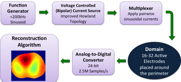
The hardware presented in this work is a pairwise current injection design. It incorporates an active electrode for acquisition of complex voltage measurements. The active complex electrode (ACE1) system contains the same basic components as most pairwise EIT systems: a current source, a tomograph box, and a voltage measurement circuit.
Figure 3.1. The basic design and acquisition of data with the active complex electrode (ACE1) system is described with this block diagram.
The components of the ACE1 system were assembled such that data is acquired in the manner described by the block diagram in Figure 3.1. To attach the system to human subjects, rectangular ECG electrodes are used (Philips 13951C neonatal/pediatric solid gel ECG monitoring snap electrodes). ACE1 is a modular system for use with up to 32 electrodes and injects currents ranging in amplitude from 0.5 mA to 5.0 mA at a discrete user-specified frequency of up to 200 kHz. During acquisition, the parallel port-controlled multiplexers ensure current is sent to the correct electrodes for injection. Electrical current spreads through the body or tank generating corresponding electric potentials on all electrodes.
Figure 3.2. The ACE1 tomograph cables connected to a human volunteer (left) and a photo of the portable system (right).
These electric potentials are buffered from noise by the active electrodes and wired to the analog-to-digital converters (ADC) in the computer. Voltages are measured on all electrodes with a 24-bit ADC at 2.5 Msamples/sec. The stored data is then processed for use in image reconstructions [75].
Shown in Figure 3.2 is the ACE1 tomograph used on a human subject and on a portable cart imaging a tank phantom. The main components include:
• the main tomograph box (contains multiplexers, direct current (DC) supply regula-tors, a logic circuit for active electrode switch control, and the current source) • cables with active electrodes that connect the tomograph to the subject or tank • analog to digital converter for 32 channels (2 GE ICS 1640 boards each with 16
channel 24-bit 2.5 Msamples/second)
• function generator (Stanford Research Systems Model DS360 Ultra Low Distortion) • DC supply for tomograph box (Mastech DC Power Supply HY3005F-3)
The ACE1 EIT system uses pairwise or skip current patterns. In this system, each frame in the dataset is formed by injecting current on two electrodes at a time and rotating the location of injection around the domain until all user-specified electrodes have acted as an injection pair. A single current pattern occurs for each instance where current is injected on a pair of electrodes. When all 32 electrodes are in use, 32 different current patterns are applied to form one frame. Potentials on all electrodes are measured during each current pattern of each frame of data acquisition.
The number of electrodes in between each of the injecting electrodes defines the skip pattern. For example, as show in Figure 3.3, in skip four, the first current injection pattern occurs between electrode one and six. The third current pattern injects current on electrodes three and eight. After each current pattern, the injection electrodes are rotated about the domain until current has been injected on all possible pairs of electrodes for a given skip pattern. Skip 4 Current Pattern i Skip 4 Current Pattern i+2
Figure 3.3. This figure illustrates the pairwise injection of current about the domain for a skip four pattern. The direction of bipolar current flow is indicated by the arrows.
In data acquisition, up to 32 electrodes can be used. Based on the number of electrodes (L) placed around the domain, some skip patterns are better for later use in the D-bar algorithm than others. In image reconstruction, it is beneficial to maintain as many linearly
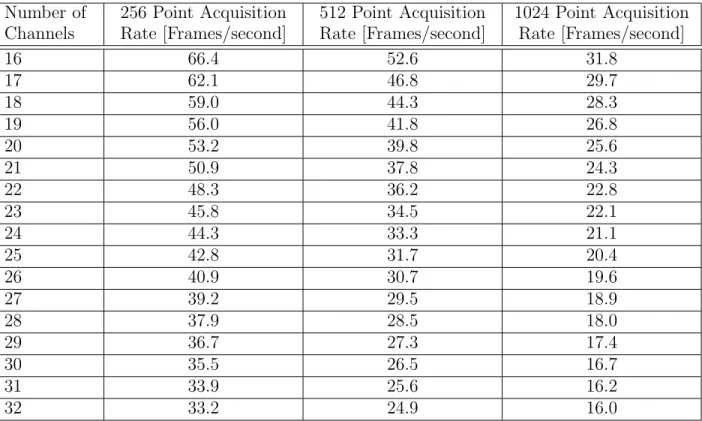
Table 3.1. Frame rates for ACE1 for varying numbers of electrodes and data point acquisition rates.
Number of Channels 256 Point Acquisition Rate [Frames/second] 512 Point Acquisition Rate [Frames/second] 1024 Point Acquisition Rate [Frames/second] 16 66.4 52.6 31.8 17 62.1 46.8 29.7 18 59.0 44.3 28.3 19 56.0 41.8 26.8 20 53.2 39.8 25.6 21 50.9 37.8 24.3 22 48.3 36.2 22.8 23 45.8 34.5 22.1 24 44.3 33.3 21.1 25 42.8 31.7 20.4 26 40.9 30.7 19.6 27 39.2 29.5 18.9 28 37.9 28.5 18.0 29 36.7 27.3 17.4 30 35.5 26.5 16.7 31 33.9 25.6 16.2 32 33.2 24.9 16.0
independent current patterns as possible. For a pairwise injection system of skip α, the number of linearly independent current patterns (N) is represented by Equation (3.1) [76]. Note that L-1 degrees of freedom is the most that can be achieved, resulting in the greatest number of voltage vectors that can be used by the reconstruction algorithm.
N = L − gcd(L, α + 1), where gcd is the greatest common divisor (3.1)
Frame rate varies depending on the number of data points or samples taken for each voltage measurement during acquisition. Table 3.1 shows various frame rates that can be achieved with ACE1. To calculate, system time stamps were saved at the beginning and end of a 500 frame data acquisition to determine the average frame rate.
![Table 2.1. Accepted values for bulk conductivity and permittivity of human tissues at 100 kHz [1–3].](https://thumb-eu.123doks.com/thumbv2/5dokorg/4332350.98181/32.918.111.808.166.453/table-accepted-values-bulk-conductivity-permittivity-human-tissues.webp)


![Figure 4.1. Improved Howland circuit model [8], where V t− = V t+ = V t when assuming ideal op amp behavior.](https://thumb-eu.123doks.com/thumbv2/5dokorg/4332350.98181/63.918.188.732.281.581/figure-improved-howland-circuit-model-assuming-ideal-behavior.webp)