Estimating the marginal costs of road wear
Jan-Eric Nilsson – VTIKristin Svensson – Dalarna University Mattias Haraldsson – Energimyndigheten
CTS Working Paper 2015:5
Abstract
Using a large set of data, including age, pavement type, traffic etc., on sections of the road network, this paper sets out to assess the marginal cost of using the road infrastructure. It suggests a strategy for identifying major differences in marginal costs across the road network, and provides evidence that not only heavy vehicles but also cars contribute to road quality deterioration. The hypothesis is that this is due to the widespread use of studded tires in countries with regular freeze-thaw cycles. No indication of deterioration due to time per se is found.
Keywords: Marginal costs, wear and tear, road reinvestment, Weibull model
Centre for Transport Studies SE-100 44 Stockholm
Sweden
Estimating the marginal costs of road wear
1Jan-Eric Nilsson,
Swedish National Road and Transport Research Institute
Jan-eric.nilsson@vti.se Kristin Svensson, Dalarna University kss@du.se Mattias Haraldsson Mattias.haraldsson@energimyndigheten.se
Abstract: Using a large set of data, including age, pavement type, traffic etc., on sections of the road network, this paper sets out to assess the marginal cost of using the road infrastructure. It suggests a strategy for identifying major differences in marginal costs across the road network, and provides evidence that not only heavy vehicles but also cars contribute to road quality deterioration. The hypothesis is that this is due to the widespread use of studded tires in countries with regular freeze-thaw cycles. No indication of deterioration due to time per se is found.
Keyords: Marginal costs, wear and tear, road reinvestment, Weibull model.
1 This paper is part of a Swedish government assignment to VTI to assess the social marginal costs of
infrastructure use; the work has been funded by an allocation from the government. We are grateful for comments on a previous version by Ken Small; the usual caveats apply.
1. Introduction
In order to maximise the social welfare from resources expended on infrastructure, two aspects are in focus. The first is to build new roads, bridges etc., once the aggregate benefits of an investment exceed the resources allocated to construction; the second is to charge for the use of existing assets according to the social marginal costs emanating from their use. The focus of this paper is on the second issue. Perry & Small (2005) demonstrate the overall scope and significance of the task.
To implement efficient charges, appropriate estimates of costs are a first requirement. This paper contributes to this research by estimating one component of the marginal cost. The purpose is to provide a model for, and a measure of, the (short-run) marginal infrastructure costs, i.e. costs related to the wear and tear of additional vehicles using the infrastructure. Thanks to an excellent set of data, it is also possible to provide differences in costs across the country, and therefore also whether or not there may be justification for differentiated pricing. The rapid development of in-vehicle positioning systems means that the system cost of
implementing differentiated pricing would be much lower today than just a few years ago.
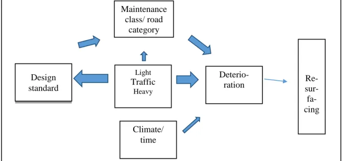
As illustrated by figure 1, meeting this challenge makes it necessary to disentangle several complex engineering interactions of road design, usage and deterioration. Traffic in the centre box is decisive for both the design standard of a new road (arrow to the left) and for the deterioration of roads, once they start to be used (rightward arrow). The more traffic that is expected on a road, the more robust is the design standard (thickness of sub- and super-structure, etc.). At the same time, the more traffic using an existing road, the faster is the deterioration.
In addition to the relevance of traffic for both design standard and deterioration, the combination of standard and traffic also provides a basis for a strategy of on-going road maintenance (the top-most rectangle). Most countries classify roads into those built for long-distance international or national traffic, or for regional or local purposes. There may, however, be sections of an international road that have little traffic, while sections of local roads may be heavily used. Moreover, irrespective of the detailed structure of road
categorisation, maintenance may be implemented in ways that have consequences for the degree of deterioration.
A further feature of the interrelationship is climate or time per se (the bottom-most rectangle), as a road surface standard may deteriorate independently of use. This is a subject where engineers do not seem to agree.
Figure 1: Interrelationship of design, traffic and deterioration of roads.
With these interrelationships as the analytical platform, the idea is that the larger the number of vehicles using a road, the more damage is inflicted on the infrastructure. Furthermore, if traffic increases relative to ex ante projections, future periodic maintenance must be advanced in time in order to retain quality. This imposes an additional cost on society, i.e. the marginal cost related to traffic, which is the focus of this paper.
A further distinction, which is not captured by the figure, concerns the relationship between vehicle weight and road wear; this association is commonly believed to be non-linear. It is therefore necessary to make a distinction between the impacts of heavy and light vehicles on road quality. The standard rule-of-thumb is that wear increases according to the fourth power of weight per vehicle axle. This rule, and the relative significance of heavy and light vehicles
Light Traffic Heavy Design standard Maintenance class/ road category Deterio-ration Climate/ time Re-sur- fa- cing
for quality and the timing of reinvestment, and therefore for estimating the marginal costs, is therefore at the core of this paper.
Previous literature: The estimation of marginal infrastructure costs, i.e. costs related to
additional vehicles using the infrastructure at large, has a long history. The emphasis in Newbery (1988) is on a very particular aspect of these estimates, namely the fact that the wear of one vehicle using a road imposes costs on subsequent vehicles using a road that then is of slightly lower quality. His fundamental theorem demonstrates that this extra cost under some assumptions, but not under others, is balanced by the date of future reinvestment being slightly brought forward in time. Marginal and average costs then coincide.
The leading model formulation for empirical analysis is the book by Small et al (1989). Their approach is also used for constructing the base model in this paper. A large number of
subsequent empirical studies, not least in the engineering field, are based on this approach. Lindberg (2006) suggested transforming this model by using the concept of deterioration elasticity in order to facilitate empirical estimations; this will be defined in more detail in section 2. In his dissertation, Haraldsson (2007) makes use of this analytical trick, and also introduces the possibility of using a Weibull distribution for estimating the life length of (sections of) the road network. Our paper provides an extension and specification of his dissertation. In addition, and making use of a unique database, we are able not only to estimate the marginal costs of road wear, but also to address some of the underlying complexities captured by figure 1.
Using the basic components of the Small et al (1989) model, section 2 specifies the analytical approach and identifies the type of data necessary for the empirical assessment. We also point out where the previous analysis is extended. Section 3 analyses the costs of re-surfacing in order to generate a measure of the average cost of resurfacing a square meter of road. Section 4 applies a time-to-event model for estimating the surface life length and the traffic using roads between the “birth” and “death” of a pavement. Section 5 present the estimation results while section 6 summarises our results.
2. The modelling framework
This section starts by developing the economic model for calculating marginal reinvestment costs (section 2.1). An essential input of this model concerns the life-length of roads, and section 2.2 describes the engineering aspects of these calculations. While these sections treat all vehicles as being identical, section 2.3 elaborates on the implications for the cost
estimation of vehicle/axle weight. Section 2.4 summarises the framework section by formulating testable hypotheses.
2.1 The economic model
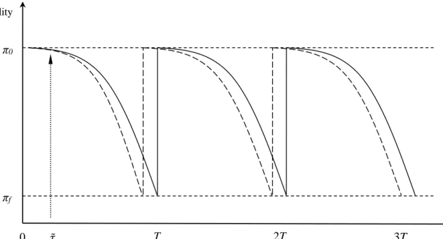
Figure 2 captures the economic framework for the reinvestment problem. The solid line denotes the reduction of quality of a piece of infrastructure as time goes by and more and more vehicles use it. At some point of time, t=T, quality reaches a critical standard (πf), and as
a result the road standard has to be restored, ideally to the original level (π0). After that, the
degradation starts once again. 2 The mirror image of this graph reflects the increasing costs of road maintenance as well as for users up to the date of renewal.
The pattern of deterioration-rehabilitation cycles is based on expectations regarding future traffic when the road is originally built. The analytical trick of the model is to assume that, at some point of time, 𝑡̃, traffic increases relative to the ex ante belief. The consequence of the unexpected (one-time) addition of traffic, and therefore also wear, is that the critical quality level will be reached slightly earlier than predicted, making it necessary to front-load the rehabilitation activity.3 Spending on rehabilitation earlier than planned represents a cost to society. Since the frontloading effect continues for the foreseeable future, the rather small cost increase in the first period may boost the present value of resurfacing substantially. The extent
2Quality is treated here as if it is a well-defined concept, which it is not. It is not necessary however to dwell on
the challenges involved in measuring quality. The assumption is simply that engineers have established some critical level of standard that triggers resurfacing. This limit value also defines the life of the pavement.
3 In order to focus the analysis, the impact of traffic growth is eliminated. In figure 2, traffic growth would mean
that the time between resurfacing intervals would gradually become shorter. Newbery (1988) deals with this by assuming a constant time interval while the rehabilitation cost increases, since more must be spent on durability (e.g. thickness of the pavement) in order to keep T constant.
of the cost increase is related to the frequency of resurfacing activities and the level of the discount rate.
Figure 2. Renewal intervals with and without a marginal increase in traffic at timet~ .
In order to model these effects, let C represent the cost per square metre of a resurfacing activity. In the absence of traffic growth, a new road surface is laid every T years. Equation (1), where r denotes the discount rate, defines the present value of all future overlay costs (PVC) at time 0.
𝑃𝑉𝐶𝑇 =(1−𝑒𝐶−𝑟𝑇) (1)
The consequences of an unexpected one-time increase in traffic at any time, τ<T, is that the present value of costs has to be discounted from the precise time of the shock, or equivalently with the number of years between the shock and today.4 Differentiating (1) with respect to annual traffic (Q) provides the marginal costs (MC). It is necessary, though, to account for the
4 Small et al (1989) use an annualized value of the Present Value Cost, i.e. r*PVC. In addition, they treat the
external change as if it happened in the same instant as when the renewal took place, and therefore use (1) rather than (1’). 2T T πf π0 Quality Time 0 𝜏̃ 3T
fact that the external shock may take place at any time between just after the pavement has been rehabilitated (at t=0) and just before the next rehabilitation (t=T). The present value of all future pavement renewal costs after 𝑡 = 𝑡̃ must therefore be discounted by 𝑒−𝑟𝜐 where
𝜐 = 𝑇 − 𝜏 is the remaining life of the pavement;
𝑀𝐶 =𝜕𝑃𝑉𝐶𝜕𝑄 = 𝜕𝑃𝑉𝐶𝜕𝑇 𝑑𝑄𝑑𝑇 = −𝐶𝑟 𝑒−𝑟𝜐 (1−𝑒𝑟𝑇) 𝜕𝜐 𝜕𝑇 𝑑𝑇 𝑑𝑄 (2)
Following Lindberg (2004), it is instructive to rewrite this expression in terms of changes in annual average traffic 𝑄; in the absence of traffic growth, 𝑄 = 𝑄. He also defines
deterioration elasticity (ε) as 𝜀 = 𝛿𝑇 𝛿𝑄
⁄ ∗ 𝑄 𝑇⁄ . This is a measure of the responsiveness in pavement life to a change in traffic intensity. The relation between a momentary traffic change and deterioration elasticity is approximately given by eq. (3); the approximation is related to the fact that a small shift in traffic intensity at time τ leads to a shift in the average traffic volume over the whole period equal to 1/T:
𝛿𝑇 𝛿𝑄𝜏= 𝛿𝑇 𝛿𝑄𝐼 𝛿𝑄𝐼 𝛿𝑄𝜏= [ 𝛿𝑄𝐼 𝛿𝑄𝜏≈ 1 𝑇] = 𝜀 𝑄𝐼 (3)
Using this, and since 𝜕𝜐 𝜕𝑇⁄ = 1, eq. (2) can be rewritten as eq. (2’).
𝑀𝐶𝜏 =𝜕𝑃𝑉𝐶𝜕𝑄 = −𝐶𝑟 𝑒−𝑟𝜐
(1−𝑒𝑟𝑇)
𝜀
𝑄𝐼 (2’)
The average MC over all possible remaining lifetimes from the date of the traffic increase, or analogously over a large number of road sections of different remaining lifetime, is the expected marginal cost taken over a probability density function of υ, g(υ):
𝐸[𝜕𝑃𝑉𝐶𝜕𝑄 ] = −𝐶𝑟𝜀𝑄 𝐼 ∫ 𝑒−𝑟𝜐 (1−𝑒𝑟𝑇)𝑔(𝜐)𝑑𝜐 ∞ 0 (3’)
If the pavement deteriorates deterministically with traffic, and the lifetime of a pavement comes to its end exactly when its quality falls to a predetermined level, g(υ) is uniform, i.e. 𝑔(𝜐) = 1 𝑇⁄ . Under this assumption, eq. (3’) collapses to the expression below, where the
expected marginal cost is equal to the deterioration elasticity times the average reinvestment cost (the quotient in the equation).
𝐸 [𝜕𝑃𝑉𝐶 𝜕𝑄 ] = − 𝐶𝑟𝜀 𝑄𝐼 1 (1 − 𝑒𝑟𝑇)[− 1 𝑟𝑒−𝑟𝜐]0 𝑇 = −𝜀 𝐶 𝑄𝐼𝑇
We assume, however, that pavement lifetime T is not deterministic. Pavement durability is modelled using a Weibull function; the reason is given in the next section. The survival function of a Weibull function implies the following pdf. for remaining lifetimes:
𝑔(𝜐) =𝑒−𝛾𝜈
𝛼
𝐸[𝑇] , 0 < 𝜐 < ∞
Substituting this into eq. (3) gives eq. (4). The first two components of this expression are the same as in the deterministic version. The third component is related to the discounting and uncertainty with respect to when in the period, between an almost new pavement (t=0) and a pavement that is about to be replaced (t=T), the external shock takes place. The fourth component allows for uncertainty with respect to when the pavement’s life ends.
𝐸[𝜕𝑃𝑉𝐶𝜕𝑄 ] = −𝜀𝐸[𝑇]𝑄𝐶 𝐼 𝑟 (1−𝑒−𝑟𝑇)∫ 𝑒 −𝑟𝜐−𝛾𝜐𝛼𝑑𝜐 ∞ 0 (4)
2.2 The engineering model
The input for calculating expected marginal costs as depicted by eq. (4) requires information about costs (C) and the life of a pavement (𝑇). Postponing the derivation of costs to section 3, this section elaborates on the engineering aspects of the problem in order to derive an estimate of average pavement life.
A road and its pavement are designed to withstand a certain number of vehicle passages before requiring treatment such as a new surface layer. As explained above, the road is resurfaced once pavement quality (π) reaches the value 𝜋𝑓 < 𝜋0. Following Small et al
depicted by eq. (5) where 𝑁 = ∑𝑇𝑡=0𝑄𝑡, i.e. the aggregate number of vehicles over the road’s
life cycle. The latter number is obviously a derivative of the quality that triggers the reinvestment, πf.
𝜋(𝑡) = 𝜋0− (𝜋0− 𝜋𝑓)(𝑄∗𝑡𝑁 )𝑒𝑚𝑡 (5)
In addition to the degree of use, the exponential part of eq. (5) indicates that pavement roughness may increase at a rate 0 ≤m≤1, which is independent of wear. With m=0, road quality is proportional to cumulative traffic (Q*t). The presence of the m-variable may represent several features. Figure 1 points out that ageing per se may affect the standard, meaning that even a road that is not used would decay. Deterioration could possibly also be affected by weather or climate, meaning that different countries may see their roads
deteriorate in different ways. These aspects will be revisited in the final discussion.
Svensson (2014) uses the semi-parametric Cox proportional hazards model where no a priori assumption of a specific distribution of the data on ageing is required. The hazard is said to be proportional, since the ratio between the hazards of two road sections with different values of one covariate is constant. Using that modelling approach, the expected life of a certain pavement or road section is not affected by when it was originally built.
Following Haraldsson (2007), we rather assume that T follows a Weibull distribution with parameters γ>0 and α>0. In this way, the precision of the estimates improves, and it will be feasible to consider the impact of the (weather) variable m in eq. (5). The Weibull distribution function (F(t)), survival function (S(t)) and hazard function (λ(t)) are represented below; the probability density function of remaining lifetimes υ was established in section 2.1.
𝐹(𝑡) = 1 − 𝑒−𝛾𝑡𝛼
𝑆(𝑡) = 𝑒−𝛾𝑡𝛼
𝜆(𝑡) = 𝛾𝛼𝑡𝛼−1
Of particular interest is the hazard function. While the hazard is not directly observable, it is equivalent to a lifetime function that can be estimated and tested empirically. In the
replaced at time t, given that it lasts so long. Following Kiefer (1988), explanatory variables can be introduced in the Weibull model using a proportional hazard:
𝜆(𝑡) = 𝑓(𝑋)𝑡𝛼−1
Replacing the exponential (weather) variable 𝑒𝑚𝑡 in eq. (5) by a power function, 𝑡𝛼−2, we get
an expression describing the deterioration of road quality over time akin to the proportional Weibull hazard:
𝜋𝑡 = 𝜋0−(𝜋0− 𝜋𝑓)𝑄𝑡𝑁 𝑡𝛼−2= 𝜋
0−(𝜋0− 𝜋𝑓)𝑁𝑄𝑡𝛼−1 (5’)
With this formulation, 𝛼>2 implies the presence of a weather effect while road quality is proportional to Q*t (cumulative traffic) if 𝛼 ≤2. It is straightforward to interpret equation (5’) as an increasing hazard indicating that the road lifetime will more probably end if it has lasted a long time. Normalizing the road quality so that initial quality is zero, 𝜋0 = 0, we get the proportional Weibull hazard:
𝜆(𝑡)=𝜋𝑓
𝑄 𝑁𝑡𝛼−1
Kiefer (1988) demonstrates that this hazard is equivalent to a log linear lifetime function. In equation (6) ϵ is a random error term following an extreme value distribution. In terms of the economic model in eq. (4), -βQ/(α-1) is the deterioration elasticity.
−∝ 𝑙𝑛𝑇 = 𝑙𝑛𝜋𝑓+𝛽𝑄𝑙𝑛𝑄 − 𝛽𝑁𝑙𝑛𝑁 + 𝜖 (6)
2.3 Light and heavy vehicles
Before deriving the information necessary for estimating eq. (4), it is necessary to elaborate on the treatment of traffic. Eq. (5’’) in combination with eq. (7) facilitates an analytical separation of heavy and light vehicles in the deterioration process. Starting with eq. (7), y is the number of days per year; using a traffic-per-day statistic is the standard way in the industry to represent traffic information. 𝑞𝑖 is the average number of vehicles of class i per day and there are i=1,…,I classes of vehicles. One of these, class j, represents passenger
vehicles while all other classes refer to different weight and axle configurations of heavy vehicles. 𝜆(𝑡) =𝜋𝑓∑ 𝜇𝑁𝑖𝑞𝑖𝑡𝛼−1 (5’’)
P a ia ia i W k y 1 4 10 * (7)𝜇𝑖 in eq. (5’’) is used for transforming the number of (heavy) vehicles in each vehicle class into “standard axles” using the universally agreed Equivalent Standard Axle Load (ESAL) concept. One ESAL is a single axle of 18 000 pounds, (8 164 kg). Vehicles in all I classes are therefore converted to ESALs. In this, a=1…P denotes the axles (or axle groups) for vehicle type i with P=8 typically being the maximum number of vehicle axles (groups).
W
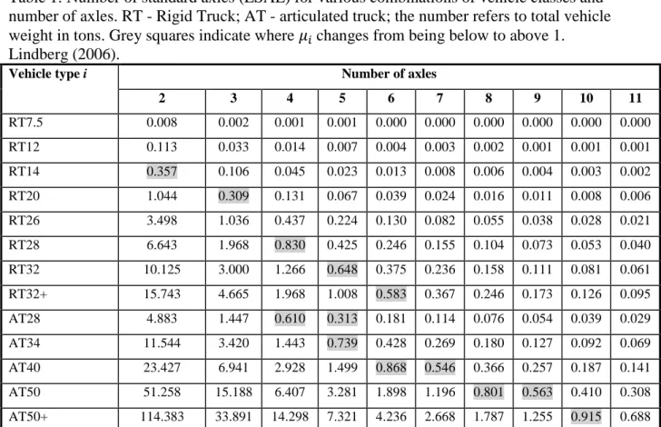
a is the weight (tons) of axle (group) a which is divided by 10 for normalisation purposes. Weight is then raised to the fourth power, meaning that an increase from 8 to 10 tonnes per vehicle axle does not increase the wear of vehicle type 𝜇𝑖 by (10/8=) 25 but by ((10/8)4=) 144 percent.In Table 1 the number of standard axles has been computed for various vehicle classes and numbers of axles using the fourth power rule. The first row represents a 7.5-ton standard Rigid Truck that has two, possibly three, axles. Irrespective of which, this vehicle’s impact is 0.002≤ESAL≤0.008, i.e. its road wear is minimal.
A 26-ton Rigid Truck has an ESAL just above one if it is equipped with three axles, while the ESAL is 0.473 if it has four axles. For each specific vehicle type, the number of standard axles decreases when the number of axles increases, since the weight per axle then decreases. Thus, a larger number of axles will cause less road deterioration for each vehicle class.
The rule per se emanates from an empirical test conducted in the US mid-west in the late 1950s. Moreover, re-estimating the original data using more up-to-date econometrics, Small et al (1987) confirm the result with a coefficient of 3.7.
While the fourth power rule-of-thumb has been challenged, no alternative has been suggested. As part of the government assignment triggering our paper, resources have been made
The testing has been done by building roads of different strengths and then wearing them down in a “lab” in order to establish when the critical quality level is reached.5 Three road
types have been tested, with type 1 being modern and well built and types 2 and 3 being of older standard. Each road type has been tested with three different weights: 8, 10 and 12 tons per axle pair. The equipment makes about 22 000 passages per full day corresponding to 150 000 passages per week. Somewhere between 300 000 to 600 000 passages are required to break down the surface – to create ruts that are large enough to warrant resurfacing.
Table 1: Number of standard axles (ESAL) for various combinations of vehicle classes and number of axles. RT - Rigid Truck; AT - articulated truck; the number refers to total vehicle weight in tons. Grey squares indicate where 𝜇𝑖 changes from being below to above 1.
Lindberg (2006).
Vehicle type i Number of axles
2 3 4 5 6 7 8 9 10 11 RT7.5 0.008 0.002 0.001 0.001 0.000 0.000 0.000 0.000 0.000 0.000 RT12 0.113 0.033 0.014 0.007 0.004 0.003 0.002 0.001 0.001 0.001 RT14 0.357 0.106 0.045 0.023 0.013 0.008 0.006 0.004 0.003 0.002 RT20 1.044 0.309 0.131 0.067 0.039 0.024 0.016 0.011 0.008 0.006 RT26 3.498 1.036 0.437 0.224 0.130 0.082 0.055 0.038 0.028 0.021 RT28 6.643 1.968 0.830 0.425 0.246 0.155 0.104 0.073 0.053 0.040 RT32 10.125 3.000 1.266 0.648 0.375 0.236 0.158 0.111 0.081 0.061 RT32+ 15.743 4.665 1.968 1.008 0.583 0.367 0.246 0.173 0.126 0.095 AT28 4.883 1.447 0.610 0.313 0.181 0.114 0.076 0.054 0.039 0.029 AT34 11.544 3.420 1.443 0.739 0.428 0.269 0.180 0.127 0.092 0.069 AT40 23.427 6.941 2.928 1.499 0.868 0.546 0.366 0.257 0.187 0.141 AT50 51.258 15.188 6.407 3.281 1.898 1.196 0.801 0.563 0.410 0.308 AT50+ 114.383 33.891 14.298 7.321 4.236 2.668 1.787 1.255 0.915 0.688
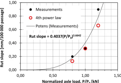
Figure 4 provides an image of the results testing the best road, i.e. type 1. The most striking observation is that the measurement results are very close to the fourth power rule-of-thumb. To be sure, the trials do not generate statistically robust results. They do, however, point to a way of taking this type of analysis one step further. Moreover, the results do not contradict the use of the fourth power hypothesis in this paper.
As well as addressing the distinction between vehicles with different weights, the rule has a clear implication for the impact of light vehicles on resurfacing decisions. A 1.6 ton car with the same weight on both axles corresponds to 6.3*10-6 ESAL. The wear of passenger vehicles of this dimension is therefore very small.
Figure 3: Rutting increase (mm/100,000 passages) as a function of normalized axle load for road type 1. From Erlingsson (2014).
There is, however, a separate discussion about passenger vehicles damaging pavements due to the use of studded tyres in countries with repeated freeze-thaw cycles. Since we have access to detailed information, it will be feasible to address the possibility that not only heavy but also passenger vehicles are of relevance for road quality deterioration. This is done by way of representing usage in terms of heavy vehicles/ESAL as well as the number of passenger vehicles in the estimation of pavement life. In equation (6), Q is then separated into Q-j and
Qj, the former accounting for average ESAL of all heavy vehicles and the latter the number of
passenger vehicles using each road section.
2.4 Summary
To summarise, eq. (4) establishes the way in which expected marginal costs relating to the impact of traffic on the need for reinvestment are to be calculated. Section 2.2 has elaborated on how road quality deteriorates over time, while section 2.3 has emphasised the need to
Rut slope = 0.4037(P/P0)3.6642 0,00 0,20 0,40 0,60 0,80 1,00 0,00 0,50 1,00 1,50 R u t sl o p e [ m m /100 000 p assag e ]
Normalized axle load, P/P0[kN]
Measurements 4th power law
distinguish between heavy and light vehicles. While the difference between vehicle types has a huge impact on the numerical outcome of the estimations, it does not affect eq. (4). The only consequence is rather that Q (and N) is not conceived of as vehicles at large but ESALs of heavy vehicles and the number of passenger vehicles.
The generation of information for estimating marginal costs as defined by equation (4) therefore means that three hypotheses are tested against available data: Quality deteriorates due to the extent of heavy vehicles, measured as ESALs (hypothesis 1), the number of light vehicles (hypothesis 2) and time, independently of the extent of traffic (hypothesis 3).
3 Calculating reinvestment costs
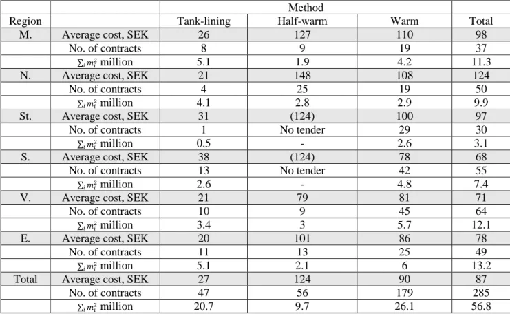
Calls for tenders regarding all maintenance and reinvestment activities are made by Trafikverket, the Swedish Transport Administration. 285 resurfacing contracts, tendered during 2012 and 2013, have been made available for deriving a value of average cost for resurfacing, i.e. C in eq. (4). Contracts range in size from just over SEK 1 million to SEK 65 million; the smallest contracts are for less than 1000 m2, and the largest for 2.2 million m2. This information has been employed to calculate the average cost for the country as a whole, as well as for each region and pavement method; cf. table 2.
Three pavement techniques, referred to as warm, half-warm and tank lining, are tendered. The average cost is derived from the observed cost for each contract and the respective contract size is measured in square meters (m2). The national average is calculated using the relative size (∑𝑖𝑚𝑖2) as the weight for region and type of pavement. In two regions, no tank-lining and half-warm contracts were tendered in 2012 and 2013. Since there are indeed roads with these qualities of pavement in these regions as well, the average for the respective category has been imputed in these cells.
Table 2: Average cost per contract in six regions and for three types of pavement. 2012 and 2013, SEK/m2. None – no contract using this method has been tendered in this region. Number within brackets has been imputed using the average cost in these cases.
Method
Region Tank-lining Half-warm Warm Total
M. Average cost, SEK 26 127 110 98
No. of contracts 8 9 19 37
∑ 𝑚𝑖2
𝑖 million 5.1 1.9 4.2 11.3
N. Average cost, SEK 21 148 108 124
No. of contracts 4 25 19 50
∑ 𝑚𝑖2
𝑖 million 4.1 2.8 2.9 9.9
St. Average cost, SEK 31 (124) 100 97
No. of contracts 1 No tender 29 30
∑ 𝑚𝑖2
𝑖 million 0.5 - 2.6 3.1
S. Average cost, SEK 38 (124) 78 68
No. of contracts 13 No tender 42 55
∑ 𝑚𝑖2
𝑖 million 2.6 - 4.8 7.4
V. Average cost, SEK 21 79 81 71
No. of contracts 10 9 45 64
∑ 𝑚𝑖2
𝑖 million 3.4 3 5.7 12.1
E. Average cost, SEK 20 101 86 78
No. of contracts 11 13 25 49
∑ 𝑚𝑖2
𝑖 million 5.1 2.1 6 13.2
Total Average cost, SEK 27 124 90 87
No. of contracts 47 56 179 285
∑ 𝑚𝑖2
𝑖 million 20.7 9.7 26.1 56.8
The average amount for contracts is SEK 87 per m2. Contracts for tank-lining are much cheaper per m2 than the other types of surfacing. This is as expected since this type is primarily used on roads with fewer than 1000 vehicles on average per day. In view of the apparent simplicity of half-warm pavements, it is less than obvious why black tops using materials defined as “warm” are less expensive per m2. One explanation is that the half-warm pavement is used on roads with intermediate traffic levels (between 1000 and 7000 vehicles on average per day) that may not have been built to standard from the beginning. If this is correct, and if a substantial number of heavy vehicles uses this class of road, the resurfacing activity in reality represents a rehabilitation project. To the extent that the cost is triggered by an inappropriate surface standard, and since contracts may have this quality, the choice has been made to use this figure in the estimations of marginal costs.
4 Estimating pavement life
Trafikverket’s Pavement Management System (PMS) is used for storing data collected during annual road-quality measurement activities. The system registers information about when a
road is “treated” in different ways, including major pavement renewals. In addition, it includes information on the traffic using each road segment. Section 4.1 provides further details of this dataset, section 4.2 describes the Weibull model used for estimating pavement life, and section 4.3 presents the results.
4.1 Data
The 2012 version of the PMS comprises 390,966 observations of homogeneous road sections. Sections vary in length, from over one kilometer to only a few meters. Only sections that are 50 meters or longer have been retained. The elimination of short sections in combination with other quality controls has resulted in 266,614 road sections for analysis.
A lot of data is available for each section; for instance, which of five different width classes the section belongs to, as well as the precise type of pavement laid, facilitating the estimation of life expectancy on a very disaggregate level. However, the previous section demonstrated that information is less abundant in terms of resurfacing costs. As a consequence, the only type of information that can be used for estimating marginal costs at a disaggregate level is three main categories of pavement spelled out by table 2. Since each of the six regions invite tenders for these contracts, 18 different cost observations are possible, resulting in the likelihood of managerial differences. Moreover, the dummy for regions may capture differences with respect to climate, the situation in the north of the country being different from that in the south. Table 3 summarizes some descriptive aspects of the data.
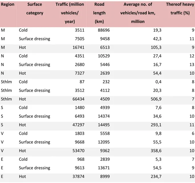
The fifth column illustrates the strong dominance of traffic on roads with the most expensive type of pavement. Svensson (2014) provides an analysis including many more covariates and also describes the way in which data has been compiled.
The final step in the handling of input data concerns the way heavy traffic is converted to ESAL. The information on this aspect is extremely poor. Since 2004, Trafikverket has collected data at 12 places across the country by using a Bridge Weigh-in-Motion system registering inter alia the number of axles and axle configuration as well as total vehicle weight. This provides a type of data appropriate for the purpose of this paper, except that 11 of the 12 measuring points are located on major roads, here represented by the “warm”
pavement technology. Only one measurement refers to a cold-type pavement; the location is close to a saw-mill and generates a non-average result; see also Erlingsson (2010).
Table 3: Descriptive statistics of traffic and road length within each region and surface category registered in 2012. Source: Trafikverket PMS system.
Region Surface category Traffic (million vehicles/ year) Road length (km) Average no. of vehicles/road km, million Thereof heavy traffic (%) M Cold 3511 88696 19,3 9 M Surface dressing 7505 9458 42,3 11 M Hot 16741 6513 105,3 9 N Cold 4351 10529 27,4 12 N Surface dressing 2680 5446 16,7 13 N Hot 7327 2639 54,4 10 Sthlm Cold 87 232 0,4 8 Sthlm Surface dressing 3512 4112 20,3 8 Sthlm Hot 66434 4509 506,9 7 S Cold 1480 4939 7,6 8 S Surface dressing 6493 14374 34,6 10 S Hot 47297 14495 293,1 11 V Cold 1803 5558 9,8 6 V Surface dressing 9668 12095 55,5 10 V Hot 53470 9362 358,6 10 E Cold 968 2839 5,3 7 E Surface dressing 9613 13671 54,5 9 E Hot 37874 8999 234,7 10
In our analysis the following values are used for converting the number of observed heavy vehicles to average ESAL: major roads with hot pavement, 1.1; cold pavement type 0.9; surface dressing 0.6 if the share of heavy traffic is below 13 percent; 1.5 if it is 13 percent or higher.
4.2 Modelling life length
In order to compute the expected present value marginal cost, it is necessary to estimate the deterioration elasticity, ε, and the Weibull parameters α and γ. As before, 𝑄̅ is the traffic volume during an average year between the year the original pavement was spread and its final year, T. Heavy traffic is represented as 𝑄𝐸𝑆𝐴𝐿 and the number of passenger vehicles 𝑄𝑐𝑎𝑟. Since neither N (the amount of traffic a road can bear before renewal) nor π(f) (the
actual, critical level of road quality), can be observed, a vector of covariates M, which may have an impact on the pavement lifetime, including a constant, is used in order to provide a consistent estimate of the traffic coefficient. A linear model is then given by eq. (8)
representing the empirical equivalent of eq. (6):
−𝛼𝑙𝑛𝑇 = 𝑙𝑛𝑄𝑐𝑎𝑟𝛽𝑄𝑐𝑎𝑟+ 𝑙𝑛𝑄𝐸𝑆𝐴𝐿𝛽𝑄𝐸𝑆𝐴𝐿+ 𝛽𝑵𝑴 + 𝑢 (8)
Estimated coefficients 𝛽𝑄𝑐𝑎𝑟 and 𝛽𝑄𝐸𝑆𝐴𝐿 are used for testing hypotheses 1 and 2 respectively. If these coefficients are significantly different from zero, they will signal the impact of heavy traffic and passenger vehicles on reinvestment costs. If so, the coefficient values may also be used for calculating the respective marginal costs. In addition, the value of 𝛼̂ is used for testing the hypothesis that there is an independent time/weathering effect on the hazard of a road being “treated”. Specifically, if 𝛼̂ > 2 the last component of eq. (5’) makes the hazard increase at an increasing rate with time. With estimates of 𝛽̂𝑄
𝑗, 𝛽̂𝑄−𝑗 and 𝛼 it is also feasible to
compute the deterioration elasticity.
𝜀̂𝐸𝑆𝐴𝐿 =𝛿𝑙𝑛𝑄𝛿𝑙𝑛𝑇 𝐸𝑆𝐴𝐿= − 𝛽̂𝑄𝐸𝑆𝐴𝐿 𝛼̂ and 𝜀̂𝑐𝑎𝑟 = 𝛿𝑙𝑛𝑇 𝛿𝑙𝑛𝑄𝑐𝑎𝑟= − 𝛽̂𝑄𝑐𝑎𝑟 𝛼 ̂ 4.3 Results
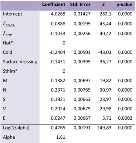
Table 4 provides the results of the estimates of eq. (7). As expected, the large number of observations enables very precise estimates. Cold surfaces and surface dressing have statistically significantly shorter lives than warm pavements. Moreover, Stockholm’s roads last a shorter time than roads in the other regions; region M roads “live” about 13 percent longer than region Stockholm roads. A possible reason is that even though roads in Stockholm are generally robustly built, the level of traffic is much higher than in the other regions.
Based on these results, hypothesis 3 is rejected while hypotheses 1 and 2 are not: Both light and heavy vehicles affect the timing of resurfacing activities and consequently the life length of pavements, but there are no aspects related to time and weather that do. Bearing in mind the crude way to transform information about heavy vehicles into ESAL, it is noteworthy that the impact of passenger vehicles on surface life is stronger than the consequences of
variations in heavy vehicles.
Our hypothesis is that the significance of the coefficient for cars can be rationalised by their use of studded tires. If this hypothesis is correct, it is reasonable to expect that the road wear of cars in the north of the country is at a lower level than in the reference, which is the
Stockholm region in the middle of the country. This is so since the road surface in the north is covered by snow and ice for longer periods than in the southern parts of the country, meaning that the studs do not wear down the pavement for equally long periods. In addition, the
southern parts of Sweden have less harsh winters than up north, with the result that fewer cars use studded tires.6 Interacting cars and regions provides an indication that these conjectures may be correct. Compared to Stockholm, the car-region coefficient is some 20 percent higher for regions North, South and West, while roads in regions East and Middle last about 10 percent longer.
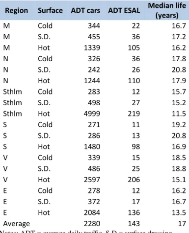
The results in table 4 are used to estimate life length based on car traffic and ESAL as
summarized in table 5. Median lifetime is strikingly similar across surface types and regions.7
Hot pavements live slightly shorter times in spite of being more robust. Most probably, the reason is that they are used by much more traffic than roads with other types of surface treatment.
6 SMHI (2008) indicates that 44 percent of cars in region South had studded tires in 2008 while the average for
the rest of the country was close to 80 percent.
7 Median life is the spot where the survival function S(t) = 0.5. The hazard function h(t), which is estimated, is
Table 4: Estimates of surface life length using a Weibull model. 252 309 observations of homogeneous road sections. * - reference category.
Coefficient Std. Error Z p-value
Intercept 4,0268 0,01427 282,1 0,0000 𝜀̂𝐸𝑆𝐴𝐿 -0,0888 0,00195 -45,44 0,0000 𝜀̂𝑐𝑎𝑟 -0,1033 0,00256 -40,42 0,0000 Hot* 0 Cold -0,2404 0,00501 -48,03 0,0000 Surface dressing -0,1431 0,00395 -36,27 0,0000 Sthlm* 0 M 0,1382 0,00697 19,82 0,0000 N 0,2371 0,00765 30,97 0,0000 S 0,1921 0,00663 28,97 0,0000 V 0,2024 0,00675 29,98 0,0000 E 0,0247 0,00667 3,71 0,0002 Log(1/alpha) -0,4765 0,00191 -249,83 0,0000 Alpha 1,61
Table 5: Lifetimes estimated from the Weibull model.
Region Surface ADT cars ADT ESAL Median life (years) M Cold 344 22 16.7 M S.D. 455 36 17.2 M Hot 1339 105 16.2 N Cold 326 36 17.8 N S.D. 242 26 20.8 N Hot 1244 110 17.9 Sthlm Cold 283 12 15.7 Sthlm S.D. 498 27 15.2 Sthlm Hot 4999 219 11.5 S Cold 271 11 19.2 S S.D. 286 13 20.8 S Hot 1480 98 16.9 V Cold 339 15 18.5 V S.D. 486 25 18.8 V Hot 2597 206 15.1 E Cold 278 12 16.2 E S.D. 372 17 16.7 E Hot 2084 136 13.5 Average 2280 143 17
Notes: ADT = average daily traffic, S.D.= surface dressing
5 Calculating marginal costs
Equation (4) is used for calculating marginal costs. In order to elaborate on the logic of the estimations, the equation is used to describe how the national average marginal cost is calculated.
C is the construction cost, which in Table 2 is SEK 87 per square meter for an average road. 𝑄 is the average annual traffic over the roads’ life cycle. The 2012 figure is 2280 cars and 143 ESAL on average per day. The pavement lasts for an average of 17 years (T). Since car traffic has increased by 1 percent p.a., it is straightforward to establish an average of 2112 cars per day over the period.8 With traffic growth at 1.8 percent p.a. for heavy vehicles, the number of ESALs is 125 vehicles per day over the life cycle. The average number of heavy vehicles and cars using the average road between its birth and death is therefore (17 years * 365 days *
125=) 776 000 ESALs and (17 years * 365 days * 2112=) 13.1 million cars. The average cost is SEK 87 divided by these numbers, i.e. SEK 1.12 * 10-4 per ESAL and 6.64*10-6 per car.
The first component of eq. (4), 𝜀, represents the deterioration elasticity, now split into two, i.e. 𝜀̂𝑐𝑎𝑟𝑠 and 𝜀̂𝐸𝑆𝐴𝐿. The numbers in table 3 indicate that increasing ESAL or number of cars by
10 percent will reduce the service life of pavements by about one percent for both categories. Multiplying the average cost by the respective elasticities, the result is (0.0888*1.12 * 10-4 =) 9.95*10-6 for ESAL and (0.1036*6.64*10-6 =) 0.69*10-6 for cars.
The official discount rate for the transport sector, r, is 3.5 percent. With median life being 17 years, the value of 𝑟
(1−𝑒−𝑟𝑇) is 0.078. The final component of eq. (4) is the integral
∫ 𝑒∞ −𝑟𝜐−𝛾𝜈𝛼𝑑𝜐
0 . This is a means for dealing with the fact that an external shock, i.e. an
unexpected increase in traffic, could materialise at any point between the previous and the next date of renewal. The value of the integral for the average road is 12.5, and the
combination of these two terms 0.976. Given eq. (4), the marginal cost estimate is (9.95*10-6 * 0.976 =) SEK 9.71*10-6 for each ESAL and (0.69*10-6 * 0.976 =) SEK 0.673*10-6 for each car.
This benchmark estimate of marginal costs is calculated per square meter although the standard way to represent traffic is by vehicle km. The average Swedish road being 6.75 m wide, and multiplying by 1 000 for conversion from meter to kilometre, the marginal cost for a heavy vehicle using an average road is (6.75 * 1 000 * 9.71*10-6 =) SEK 0.066 per ESAL km and (6.75 * 1 000 * 0.673*10-6=) SEK 0.0052 per km for cars.
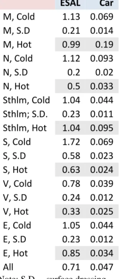
While this numerical example is based on an average vehicle using an average road, the detailed calculation of marginal costs is based on about 250 000 observations, one for each road section. In this, all road sections are given a weight based on length relative to total road length in order to create a total average. This is the approach used to derive all values in table 6. Comparing the last row in table 6 with the manual average calculated in the above example, it is obvious that the values in the table are much higher. The reason is that these numbers provide better accuracy, accounting for actual road length rather than (implicitly) assuming all links to be equally long.
Table 6: Marginal cost, SEK per ESAL kilometre and SEK per car kilometre. ESAL Car M, Cold 1.13 0.069 M, S.D 0.21 0.014 M, Hot 0.99 0.19 N, Cold 1.12 0.093 N, S.D 0.2 0.02 N, Hot 0.5 0.033 Sthlm, Cold 1.04 0.044 Sthlm; S.D. 0.23 0.011 Sthlm, Hot 1.04 0.095 S, Cold 1.72 0.069 S, S.D 0.58 0.023 S, Hot 0.63 0.024 V, Cold 0.78 0.039 V, S.D 0.24 0.012 V, Hot 0.33 0.025 E, Cold 1.05 0.044 E, S.D 0.23 0.012 E, Hot 0.85 0.034 All 0.71 0.047
Note: S.D. – surface dressing
The only point of reference that can be used for benchmarking these results is Haraldsson (2007); his aggregate estimates are SEK 0.01 for heavy vehicles and 0.001 for cars.9 This means that our cost estimates are higher than before. One reason may be that heavy traffic is transformed here from number of vehicles to ESAL, which was not the case in his study. Another difference is that elasticities are now 0.09 and 0.10 while they were 0.04 and -0.052 in Haraldsson (2007) for heavy and light vehicles, respectively, i.e. they are now twice as large.10 Moreover, we use more than twice the number of observations. Finally, although
both studies are based on information from the same source, seven more years of observations are now available. We have seen in other similar studies that there may have been a change in
9 The costs used in Haraldsson (2007) are based on a reference from 2004. Assuming that the cost per m2, which
is SEK 65, refers to year 2000, and using CPI, the corresponding number for 2012, which is the year used here, is SEK 78. Since the cost for asphalt has increased much faster than consumer prices, this compares well with the value used here, i.e. SEK 85 per m2.
maintenance methods over the years, which may have consequences for elasticity estimates. It would require further analyses to sort out these differences.
6. Summary
This paper has estimated the marginal costs for road reinvestment using information at a very disaggregate level. One robust result of the analysis is that not only heavy vehicles, but also light vehicles, affect the periodicity of resurfacing activities. Most probably, this is the consequence of the use of studded tires in a country with freeze-thaw cycles.
The impact of heavy vehicles on road standard varies across the country and with respect to the type of pavement used. The observation in table 5, that the cost for heavy vehicles using roads with (cheap) surface dressing (S.D.) is low, does not indicate that trucks should be induced to use these roads. Rather, and referring back to the complex interactions depicted by figure 1, it provides support for the appropriateness of the design decision to use low-cost pavements on roads not used by many (heavy) vehicles.
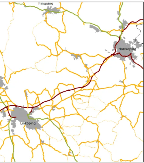
The use of disaggregate data also makes it possible to map results in the way illustrated by figure 4. The most striking observation is that the thickness of the lines/roads does not vary very much between roads in brown and green, and that many (while not all) roads in yellow are of similar thickness. This indicates that marginal costs are at a comparable level even though the level of traffic on roads in brown – the Europe roads – is much higher than on other roads. This observation is driven by the fact that fewer vehicles use roads with a cheaper type of surface treatment. Europe roads are much wider, have a more expensive type of
asphalt, and are used by many more vehicles. Average and marginal costs for using these roads are therefore kept at a level that is similar to the cheap, low-traffic roads due to scale economies.
All results of our analysis refer to an average heavy vehicle. By using Table 2 it is
straightforward to generalize these results in order to estimate costs for each combination of vehicle weight per axle and to calculate a marginal cost for each category of heavy vehicle. This should, however, be done with due respect for the meagre information available on the actual weight of vehicles.
While both trucks and cars have an impact on the timing of resurfacing, the analysis has not provided any indications of that time per se is of separate relevance for life length. One possible reason is that vehicle wear triggers the resurfacing activity long before the passage of time has any effects on the aging of the road surface.
Europe road Brown National road Green District roads Yellow
Figure 4: National roads around two cities in middle Sweden. The thickness of a line indicates the marginal cost of wear and tear, with thin roads indicating low costs.
However, it is also reasonable to ask what aspects, other than vehicle wear, are of relevance for understanding the complex relationships illustrated by figure 1. Turning the question upside down: if a doubling of traffic does not reduce the lifetime of the pavement by 50 percent, what are the decisive factors for road deterioration?
Based on World Bank research in developing countries during the 1960s, Newbery (1988) discusses different reasons for road quality deterioration. Contrasting his observations with
the outcome of the present analysis may imply that roads deteriorate over time and due to weather and climate in different ways in cold and warm climates.
It is also important to acknowledge that the heterogeneity across sections of roads is only partly characterised by available data. In particular, very little is known about the quality of the road beneath the top layer. The “life” of roads that are classified in the same way and are used by a similar number of vehicles may still differ substantially, due to the fact that they are built on solid rock, or on sand, or on materials that are not robust during the spring thaw. Constructions may also differ simply because of different skills of the construction teams or because the sub-structures built long ago had a lower standard than today. While information is abundant about surface structure, the variation in substructure still leaves the analyst with only partial information of what drives quality deterioration.
One implicit observation of this underlying heterogeneity is that half-warm pavements are actually more expensive per square meter than warm mixes. This is contrary to the fact that the half-warm mix in isolation is cheaper than the warm mix. The blip in cost data most probably indicates that the half-warm type is spread on roads that are not built for the traffic they are actually carrying. As a result, resurfacing of these roads requires more extensive rehabilitation activities, increasing the average (and marginal) costs.
In addition to the impact on rehabilitation, variations in traffic may also affect the spending on maintenance. This possibility is addressed by Haraldsson (2007) and is updated by Swärdh & Jonsson (2014) in a study that is parallel to this one. In addition, Anani & Madanat (2010) consider the possibility of activities which are more intense than day-to-day maintenance, but less so than complete resurfacing. This could, for instance, be substantial pot-hole mending or other activities with a possible impact on the timing of future resurfacing. This type of activity possibly represents a component of marginal costs, which may affect the analysis of observed life cycles and in that respect represent an additional source of (unobservable) heterogeneity. As a consequence of poor availability of data on these types of activities, it is impossible to extend the analysis in this direction.
References
Anani, S. B., S. M. Madanat (2010). Estimation of Highway Maintenance Marginal Cost under Multiple Maintenance Activities. J. Transp. Engineering, Vol. 136, Issue 10 (October), pp. 863–870
Erlingsson, S. (2010) “Characterization of heavy traffic on the Swedish road network,” Proceedings of the 11th International Conference on Asphalt Pavements, Nagoya, Japan, 01 – 06 August, CD-ROM.
Erlingsson, S. (2014) ”Tunga trafikens samhällsekonomiska kostnader – Accelerade tester av tre vägkonstruktioner,” VTI-notat, 22 s. Utkast.
Haraldsson, M. (2007). The Marginal Cost for Pavement Renewal – a Duration Analysis Approach. In Essays on Transport Economics. Dissertation in Economics, Uppsala University.
Hosmer, D., Lemeshow, S., and May, S. (2008). Applied survival analysis: Regression modelling of time-to-event data. 2nd Edition, Wiley, Hoboken, NJ.
Kiefer, N (1988). Economic Duration Data and Hazard Functions, Journal of economic literature, Vol. 26, 649-679
Lindberg, G. (2006). Development path of HeavyRoute systems – impact and socio-economic consequences. Deliverable 4.2 for EU Specific Targeted Research Project “HeavyRoute”. Newbery (1988). Road User Charges in Britain. Economic Journal, vol. 98, pp 161-176. Small, K.A., Winston. C., and Evans, C.A. (1987). Road Work. Washington. The Brooking Institute.
Parry, Ian W. H., and Kenneth A. Small. 2005. "Does Britain or the United States Have the Right Gasoline Tax?" American Economic Review, 95(4): 1276-1289.
SMHI (2008). Vintervägar med eller utan dubbdäck. (Winter roads with and without studded tires; in Swedish). SMHI note 134.
Swärdh, J-E., L. Jonsson (2014). Marginal Cost of road operation and maintenance - Swedish estimates based on data of 2004-2012. Working Paper
Svenson, K. (2014). Estimated Lifetimes of Road Pavements in Sweden Using Time-to-Event Analysis. Journal of Transportation Engineering, 140(11): 0414056.
Appendix
Table A1 shows the difference in expected median lifetime between the parametric Weibull model and the semi-parametric Cox Proportional Hazards model. While the Weibull model can be specified to model the (logarithm of the) lifetime, the Cox model is semi-parametric in the sense that the hazard 𝜆(𝑡) is not specified to any particular parametric shape. Median lifetimes from the Weibull model can be obtained through prediction because the hazard has a particular shape and log(lifetime) can be modelled directly.
The Cox model rather models the hazard in the following way: 𝜆(𝑡) = 𝜆0(𝑡)exp (𝑋𝛽)
To get estimates of the median lifetimes from a Cox model, a non-parametric estimate of the baseline hazard ℎ0(𝑡) must be used, for example through:
𝜆̂0(𝑡) = 𝑑𝑖
∑𝑘∈𝑅(𝑡𝑖)exp (𝑋𝑘𝛽̂)
where 𝑑𝑖 is the number of events at time 𝑡𝑖 and 𝑅(𝑡𝑖) is the set of individuals that could experience the event of interest at time 𝑡𝑖. The 𝛽̂-estimates are obtained through maximization of a partial likelihood (Hosmer et al. 2008). The median lifetimes are found where the
survival function 𝑆(𝑡) = 0.5; the survival function is found by its relationship with the hazard function:
𝑆(𝑡) = exp (−Λ(𝑡))
where Λ(𝑡)is the cumulative hazard function, derived by integrating over the hazard: Λ(𝑡) = ∫ λ(u)𝑑u𝑡
0
The table demonstrates that lifetimes estimated from the Weibull model are 0.5-2.2 years longer than those from the Cox model. This is due to the parametric form of the hazard specified in the Weibull model, which makes a stronger assumption about the remaining lifetime of the censored observations. With a large share of censored observations, the Cox model is more likely to underestimate the lifetime, while the Weibull model might
overestimate it depending on how close the real hazard is to the assumed Weibull hazard. This indicates that the underlying “actual” life of a surface lies within a rather narrow interval.
Region Surface Type ADT Light Traffic ADT ESAL Median Age Weibull Median Age Cox Difference (years) M Cold 344 22 16.7 15 1.7 M S.D. 455 36 17.2 16 1.2 M Hot 1339 105 16.2 15 1.1 N Cold 326 36 17.8 16 1.8 N S.D. 242 26 20.8 20 0.8 N Hot 1244 110 17.9 17 0.9 Sthlm Cold 283 12 15.7 14 1.7 Sthlm S.D. 498 27 15.2 14 1.2 Sthlm Hot 4999 219 11.5 11 0.5 S Cold 271 11 19.2 17 2.2 S S.D. 286 13 20.8 19 1.8 S Hot 1480 98 16.9 16 0.9 V Cold 339 15 18.5 17 1.5 V S.D. 486 25 18.8 17 1.8 V Hot 2597 206 15.1 14 1.1 E Cold 278 12 16.2 14 2.2 E S.D. 372 17 16.7 15 1.7 E Hot 2084 136 13.5 12 1.4