Determinants of the Economic Growth in Mexico : An Exogenous Growth Model

J

I

B

S

JÖNKÖPING UNIVERSITY

D e t e r m i n a n ts o f t h e E c o n o m i c

G r o w t h i n M e x i c o

An Exogenous Growth Model

Paper within ECONOMICS

Author: JOSÉ LUIS CASTRO

Tutors: JOHAN KLAESSON, HANNA LARSSON Jönköping DECEMBER 2008

Bachelor’s Thesis in Economics

Title: Determinants of the Economic Growth in Mexico – An Exogenous Growth Model

Author: José Luis Castro

Tutors: Johan Klaesson, Hanna Larsson Date: 2008-12-18

Keywords: Exogenous Growth, Augmented Solow Model, Human Capital, Physical Capital, Effective Labour, Mexico.

JEL Classifications: B22, C22, D24, E22, E23, J24, O47

Abstract

This bachelor thesis aims to uncover the determinants of the economic growth in Mexico with an exogenous growth model. The study is based in an Augmented Solow Model em-ployed by Mankiw, Romer and Weil in "A contribution to the Empirics of the Economic Growth” (1992). The model uses annual data of Mexico from 1960-2007 and the regressions and tests are developed in the econometric package Stata 10 for eight different periods. The thesis not only uses the Effective Labour and Physical Capital as Inputs in the production Function, but also employs the variable of Human Capital as an economic determinant of growth in the production function. The results of the model correspond with the actual scenario in Mexico; more weight to the Effective Labour (76.34%) rather than to Human Capital (2.12%) or Physical Capital (21.54%) as determinants of growth.

Table of Contents

Abstract ... i

1 Introduction ... 1

1.1 Purpose and Limitations ... 1

1.4 Outline ... 1

2 Background ... 2

3 Theoretical Framework ... 3

3.1 Earlier Studies ... 3

3.2 The Simple Solow Model ... 3

3.3 Augmented Solow Model ... 5

4 Empirical Application ... 9

4.1 Estimation ... 10

5 Results ... 11

5.1 Growth Accounting ... 15

6 Conclusions ... 18

6.1 Suggestions for Further Research ... 20

References ... 21

Appendices ... 23

List of Figures

Figure 5-1 Variables of the Model ... 11

Figure 5-2 Variables per unit of Effective Labour ... 12

Figure 5-3 Investment in Human Capital ... 12

Figure 5-4 Savings in Physical Capital ... 13

Figure 5-5 Variables in the Intensive Form ... 13

Figure 5-6 Growth Contribution by Economic factor and Period ... 15

Figure 5-7 Steady State and Accumulation of the Physical Capital ... 16

Figure 5-8 Steady State and Accumulation of the Human Capital ... 16

Figure 5-9 Estimated Production Functions by Period ... 17

Figure 5-10 Production Functions vs Physical and Human Capital ... 18

List of Tables

Table 5-1 Results of the Estimated regressions for each period ... 14

1

Introduction

Throughout the world economic history, one factor that has caused discussion has been the economic growth. This phenomenon has not been the same in all countries and much less constant over time. Today, there are numerous theories that have tried to find the main determinants of economic growth. Nevertheless, the economies are so complex that it is difficult to take into consideration each and every one of the factors that generates it. According to the Central Bank of Mexico, over the past 25 years, Mexico has experienced an average GDP growth of 2.8% (Banxico, 2008), while the economies of the Newly Indu-strialized Countries (NIC), such as China, have grown 9.7% on average. In contrast, the World Development Indicators published by the World Bank, shows that the developed countries such as England and Japan have grown on average 2.3% and 2.4% respectively. However, if we examine the growth in the last 25 years of the GDP per capita (GDP pc) for Mexico, China, Britain and Japan, this is 20.7%, 675%, 72.3% and 64.8% respectively (World Bank, 2008). Therefore, it is possible to see that when the growth is viewed from this perspective, the increase in Mexico’s GDP is substantially lower compared to devel-oped countries and of course to China.

Thus, because of this situation it is possible to observe that one aspect that explains the economic growth of countries is the population growth. The rates of population growth in Mexico, Japan, Britain and China in the last years have been 1.7%, 0.1%, 0.3% and 1.1% respectively (World Bank, 2008). But, is not China the most populous country in the world? Yes, and that is why we must also take into consideration other important aspects or factors, such as Capital Accumulation, Investment in Human Capital, and so on. Just in the same period of analysis, Mexico has increased, its accumulated capital, in 3.5% on aver-age, while China has increased it in 11.8% (World Bank, 2008).

The actual world financial crisis is causing that in the next years most of the economies do not even grow. Mexico is not safe from this crisis. For this reason it is important to study the main factors that generate growth and development in order to determine the decisive actions to be taken by Mexico.

1.1 Purpose and Limitations

This paper will attempt to explain the determinants of economic growth in Mexico during the period 1960-2007 in order to establish policies this country must follow . The study will be based on the growth model exhibited by Solow in 1956 and adopts a function of in-creased production employed by Mankiw, Romer and Weil in "A contribution to the Empirics

of the Economic Growth” (1992).

1.2 Outline

The paper is structured as follows; first a Theoretical Framework, in which the basic model and early studies on this field will be reviewed. After this analysis, a background in the economic history of Mexico will be presented, in order to relate it with the results of the model in the period analyzed. The following section will explain the model employed and its assumptions and properties. Once the model is structured, the results will be pre-sented and analyzed one by one to compare it with the economic situation in Mexico. Fi-nally the paper will end with the conclusions and suggestions for further research.

2

Background

In the 1950s and part of the 1960s, Mexico experienced a remarkable economic growth, thanks to the “Stabilizer Development” model. In the 70's, the government decided to im-plement policies of aggregate demand by increasing their participation in the economy through public deficit spenditure, causing inflation and increasing the deficit in the external sector (Aspe, 1993).

The last part of the 70’s was carried out by the devaluation of the peso, which was an over-due policy, generating a huge debt in Mexico. Only in the six-year term of Lopez Portillo’s presidency governance (1976-1982), Mexico's external debt increased from 26 billion to 80 billion dollars and the Mexican peso depreciated from $22 to $70 per dollar (Krauze, 1997). Later, in the 1980s, the economic growth was indeed worthless because it was a time of po-litical imbalance, economic destabilization, declining trade and inflation disparity. So, the Mexican government implemented a series of policies set by the International Monetary Fund (IMF) which generated a “Structural Adjustment” in the public sector.

This economic model was adopted by Mexico after the crisis of 1982. The origin of the cri-sis went back to the late sixties and was due to exhaustion and breakdown of the mode of state-monopoly regulation in force since the postwar period of the Second World War (Agudelo, 1997).

During 1970-1982, 883 public companies were created; by the end of this period most of them were already in bankruptcy, so, as part of the economic reform, the government pro-posed selling them, that is, moving towards privatization (Aspe, 1993).

The primary objectives of this neoliberal model were based on the following points:  The deliberate contraction of public spending and money supply.

 The liberalization of prices, interest rate and exchange rate.

 The battle against inflation, financial stability and strengthening domestic savings.  Streamlining and relaxation of the protectionist policy of foreign trade (greater

openness to foreign trade, ie, exports and imports).

In 1987 there was hyperinflation in the country caused by the huge foreign debt, so the government, corporations, labor unions and business leaders made a "pact" in which all ac-cepted not to raise prices to curb inflation.

During the period 1989 – 1994, the total foreign investment was of 94,691 million dollars, of which 29.2% (27 705 million dollars) were Foreign Direct Investment and the remaining 70.8% (66,986 million) was channeled to the stock market, so, the real interest rates dropped substantially (Krauze, 1997).

Moreover in the 90's the banking privatization caused a domestic debt overhang, due to the release of financial activity and the removal of the legal reserve, generating an increase of the interest rates of loans. This caused a problem for banks of insolvency of portfolios of overdue loans and unpaid payments by businesses.

In late 1992, the restrictive monetary policy caused the slowdown in the economy and wea-kened the financial system, aggravating the problem of overdue loans.

In 1994 Mexico implemented a rescue plan of 40 billion dollars financed by U.S. President Bill Clinton and the IMF to resolve the crisis. However, this action increased substantially Mexico's external debt in the next year, to $ 158 million dollars (Agudelo, 1997).

During recent years Mexico has had a fairly stable economic policy thanks to the autonomy that the Central Bank enjoys. The government has pursued a policy of low public deficit, which is approximately between 8% and 15% (INEGI, 2001). Moreover, Mexico has re-mained open for trade.

3

Theoretical Framework

3.1 Earlier Studies

Several studies have been conducted within the economic growth. The conventional growth theories are based on international trade and in the comparative advantage as a source of growth. The first economist that discuss this was David Ricard in 1817 with “Principals of Political Economy”. During the second half of the twentieth century the theories on economic growth changed, mainly by the work of Solow in 1956.

These theories have been evolving during the last three decades, giving as a result the theo-ries in Exogenous Growth. These studies determined that any economy can grow without the necessity of an exogenous factor, so every country can grow by just saving or investing in new technologies or in reproducible factors, like the Human Capital. The main author in this theory is Paul Romer, who in 1986 wrote the paper “Increasing returns and long-run

growth”. Romer created a model that included the Knowledge as Input in the Production

Function (Learning by Doing).

Other important contributions in the field of Exogenous Growth have been made after Romer’s work. It is important to mention the study of Robert Lucas (1988) “On the

mechan-ics of development planning” in which the author showed that the Technological Factor is

com-posed by an exogenous factor and an exogenous factor, according to the interaction be-tween the Human Capital and the technological change.

The Solow growth model, is one of the most simple and complete exogenous growth models that can easily explain this event. Different applications and approaches have been realized by different economists with this model. One of the most important contributions to the economic growth theory is the Augmented Solow Model developed by Mankiw, Romer and Weil. This paper was named A contribution to the Empirics of the Economic Growth, published in the Quarterly Journal of Economics in 1992. Such model will be used in this paper in order to study the determinants of the economic growth in Mexico.

3.2 The Simple Solow Model

The simple Solow model, developed by Robert Solow in 1956, is a neoclassical model of supply in which the market issues are absent. In this model the savings are equal to the in-vestments and the law of Say1 _{is verified.}

The production of the economy depends on the Physical Capital (K), Labour (L) and the knowledge or productivity (A). The variable A multiplied by L, generates a variable that shows the production with a certain level of knowledge and labour, known as: Effective Labour. This type of production function is identified as Harrod- Neutral, which means that is labor augmenting and this is the only type of technical progress consistent with a

stable steady state ratio. The production function presents Constant Returns to Scale, im-plying that no more benefits can be achieved by specializing.

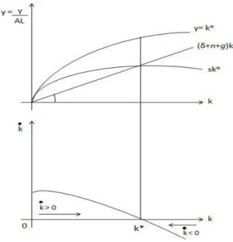
The main equation of the Solow Model denotes that the growth rate of the physical capital is the difference between the proportional production invested in capital and the growth in employment (n), productivity (g) and depreciation (δ) as a proportion of the physical capital. It is important to mention that in the Solow model these three last variables are considered exogenous. This means that the values of these variables are not determined in the model. Graphically, it is possible to observe in Figure 3-1 how this model converges to a steady state:

Figure 3-1 Solow Growth Model

The variable k* represents the optimal level of the physical capital per unit of effective la-bour. This is the value at which the economy converges in the long run.

It could be observed in the graph that if the investment in physical capital (sf(k)) is higher than (n+g+δ), k is at the beginning lower than the optimal level of physical capital (k*). So that the growth in this variable has a positive value and in consequence the physical capital increases. In the other hand, if the investment in physical capital is lower than (n+g+δ), the reverse will occur.

If k<k*, the marginal productivity of the capital is equal to the interest rate and this is high-er than the effective depreciation rate of the stock of capital phigh-er unit of Effective Labour. Therefore the economy is in lack of capital.

Further, if k<k*, also the marginal productivity of the Labour is equal to the wage (w), which would be lower than the wage of equilibrium (w*).

This principle may explain clearly the way in which the emerging countries or Newly Indu-strialized Countries (NIC) grow. This is because when their economy is located at the left of the steady state, the marginal productivity of the capital tends to be higher and in conse-quence they grow at higher rates. Nevertheless, as the economy gets close to the steady state, it will experience a constant growth rate equal to the rates of the employment growth

(n) and productivity (g). This is clearly the example of the developed countries such as Eng-land, Japan or Sweden.

3.3 Augmented Solow Model

The model that will be used to study the economic growth in Mexico in the last decades will be an Augmented Solow model. This model does not only consider that the produc-tion is given by the Physical Capital (K) and the Effective Labor (AL), but it also considers one more variable: the Human Capital (H).

Thus, the production function is:

t t t t t

K

H

A

L

Y



This equation is in the Cobb-Douglas form with Constant Returns to Scale (α+β=1) and expresses that the Production (GDP) is in function of the Physical Capital (Investment), the Human Capital (Investment in Education) and the Effective Labour (Productivity or Technology). In this paper, the technology is understood as the average of years of school-ing of the Employed Population.

The assumptions considered for this model are:

i. The technological progress (A), measured by the efficiency of the labor. Is exogen-ous and grows at the rate g.

g A

A



ii. The growth of the Economically Active Population, which grows at a constant rate

n.

n L

L



iii. The saving rate (s), which determines the equilibrium at the steady state at the ba-lanced growth path.

It is now proceeded to verify that the augmented model complies with the properties men-tioned by the simple Solow model in 1956:

 Constant Returns to Scale:

     

AL

H

K

Y

AL

H

K

Y

cAL

cH

cK

Y

 Production Function in the Intensive Form:                            1 1 AL AL AL H AL K AL Y AL c If: y AL Y _ , k AL K _ & h AL H _ :   h k y … [2]

The function in the intensive form shows us the Production per unit of Effective Labour.  Positive Marginal Productivity of the Physical Capital (PMK):

0 1     _   h k k y

 Positive Marginal Productivity of the Human Capital (PMH): 0 1     _   h k h y  Concavity: 0 ) 1 ( 2 2 2      _{ }   h k k y , because:



The concavity property proves that this model satisfies Ricardo’s Law of the Diminishing Marginal Returns.

 Satisfies the Inada Conditions:

0

lim

lim

lim

lim

These conditions are telling us that the PMK and PMH are high when the stock of physical capital and/or human capital is small enough. As far as they become smaller these marginal productivities tend to move towards infinity. So, in this model, the evolution of the econ-omy in the long run is also assumed to move to infinity (Romer, 2006).

 Variation in the Acquisition of Physical Capital: K Y s K  _k   0s_k 1

This equation is showing that the growth in the Physical Capital, throughout the time, de-pends on the savings on this factor (s_k) as a percentage of the Total Production, GDP (Y), minus the depreciation (δ) as a percentage of the Total Physical Capital, Investment (K).

 Variation in the Acquisition of Human Capital:

H Y s H  _h   0sh 1

This equation is showing that the growth in the Human Capital depends on the savings on this factor (sh) as a percentage of the Total Production, GDP (Y), minus the depreciation

(δ) as a percentage of the Total Human Capital, Investment in Education (H).

In the model with Human Capital, a distinction must be done between the Physical Capital saving (sk) and Human Capital saving (sh). So that the Total Investment (I) for this

econo-my, in terms of both savings, becomes:

I Y s s I Y s s Y I Y s s Y I C Y h k h k h k             ) ( ) 1 ( ) 1 (

On the other hand, it is also important to establish that the rates of depreciation of both factors are different, because the physical capital is depreciating at a rate higher than the human capital. However, for this model we will use a single depreciation rate for both va-riables, given by the average of both rates (Mankiw, et al; 1992).

In the Solow model, does not matter the starting point as the economy converges to a ba-lanced growth path, where each variable grows at a steady rate. This state is considered as the equilibrium of the economy in the long term.

The two fundamental equations of the model are:

A A AL KAL L L AL KAL AL K k A A A AL KL L L L AL KA AL K k A AL KL L AL KA K AL k A A k L L k K K k k AL K k                                                2 2 2 2 2 2 1

) ( ) (                  g n AL K AL Y s k g n AL K AL K Y s k g AL K n AL K AL K k k k k g n y s k  _k (  )  … [3]

In this equation [3] it is possible to see how the stock of physical capital increases due to investments in physical capital (sk) and decreases with respect to the rate of growth in the

employed population (n), technological progress (g) and depreciation (δ). The second fundamental equation of the model is:

AL H h h g n y s h _h (  )  … [4]

Similarly, the human capital increases due to investments in human capital (sh) and

decreas-es with rdecreas-espect to the rate of growth in the employed population (n), technological progrdecreas-ess (g) and depreciation (δ).

In the steady state: 0



k and 0



h , because these variables grow at a constant rate. There-fore, if we substitute these values in the equations [3] and [4] we have the optimal values (*) of k and h in the steady state:

) ( 0 ) ( ) ( 0 ) ( * *                     g n y s h h g n y s g n y s k k g n y s h h k k

After replacing and applying the properties of logarithms to the production function in its intensive form [2], the equation ends as follows:

















It is important to mention that when we estimate this equation we assume that the econo-my, although is not in the steady state, it is in the balanced growth path (Temple, 1998).

4

Empirical Application

To further explore the economic growth of Mexico and to empirically verify the economic history of Mexico, the Solow model in its augmented form will be used, which will be ap-plied to Mexico in the period 1960-2007 with annual information seasonally adjusted (thousands of Mexican Pesos 1993).

The database was compiled from different statistical bases for different periods. So were used series from the National Accounts (INEGI), the Central Bank (Banxico), Public Fin-ances of the Ministry of Finance in Mexico, the Mexican Economy in Numbers (Nafinsa), the Economic Comission for Latin America and the Caribbean (ECLAC), the Organisation for Economic Co-operation and Development (OECD), the World Bank, the Penn World Tables and the International Monetary Fund.

The variables of the model are as follows:

 Average of years of schooling of the Employed Population [A_t]  Employed population [L_t]

 GDP in thousands of pesos of 1993 [Yt]

 Gross Fixed Capital Formation in thousands of pesos of 1993 [Kt]  Public Spending on Education in thousands of pesos of 1993 [Ht]  Growth rate of the employed population [η]

 Growth rate of the average of years of schooling of the Employed Population [g]  Rate of depreciation of the physical and human capital [δ]

 Years 1960-2007 [t_t]

Again, the regression model is as follows:

















Employed Population=(Economically Active Population_t * (1-Unemployment Rate_t)

Regarding to the variable of Physical Capital (K), Mexico do not have reliable data of stock of capital, for this reason was used the Gross Fixed Capital Formation as K.

The growth rates of the employed population and years of schooling were computed as fol-lows: n L

L

_ln

_L

_ln

_L

_t

g A

A

t

A

A

_ln

_ln

In order to work with the Augmented Solow Model, first the exogenous variables, n, g & δ must be calculated. These variables are needed in order to compute the final variables that will be used in the regressions of the Augmented Solow Model.

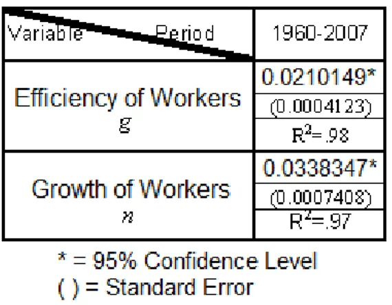
For the growth of employment (n) and the years of schooling (g) the regressions were esti-mated by Ordinary Least Squares (OLS) of the logarithmic functions mentioned above and the obtained results are presented in Table 4-1:

Table 4-1 Regression Results for Exogenous Variables (g & n)

The estimated parameters were statistically significant at a 95% confidence level. So, the ef-ficiency of workers (g) increases at a 2.1% rate and the worker’s growth rate (n) increases at a 3.38% rate.

To obtain the total rate of depreciation were used the series of Consumption of Fixed Cap-ital to obtain the relationship with respect the GDP. After that, was computed the average of the period analyzed. It was observed, according to data of the National Accounts of Mexico for the period analyzed, that the average depreciation of physical capital is 10.48%. The estimation of the depreciation of human capital is a little bit of a complicated and complex analysis. In the study of Mankiw, Romer and Weil (1992) they opted for a com-mon depreciation of human capital of 1.5%. The average depreciation for Mexico in this model, considering the Human depreciation of 1.5% and the physical capital depreciation rate of 10.48%, is then 6%.

4.1 Estimation

After the exogenous variables of the model are determined it is possible to compute the de-terminants of the economic growth in Mexico by the equation [6]. It is important to men-tion that the variables involved in this equamen-tion, are computed with the results of the ex-ogenous variables: n, g & δ. For this reason was important to first have the exex-ogenous va-riables of the model and after that work with the Augmented Solow Model.

The estimate of the equation [6] was done by the method of OLS for different periods; such regressions were estimated with the econometric package Stata 10. Since the estima-tion was done by OLS, an estimate linear equaestima-tion was obtained as follows:









t s s

y ln ln

Where:                       1 1 2 1

So, at the end remains a system of equations with two variables and it is possible to find its original values and get the rates of the original coefficients.

5

Results

The variables used in the model can be seen in the Figure 5-1. The data is seasonally adjusted for the analysis and according to the Figure 5-1 it is possible to observe how the Human Capital or Investment in Education has not grown significantly in the time. This is a fundamental factor that leads into a lower growth rate of the economy, rather than if it was at least higher.

0 5 .0 0 e + 0 81 .0 0 e + 0 91 .5 0 e + 0 92 .0 0 e + 0 9 T h o u a n d s o f Pe so s 1960 1970 1980 1990 2000 2010 Year GDP (Y) Labour (L)

Effective Labour (AL) Physical Capital (K) Human Capital (H)

Variables

Figure 5-1 Variables of the Model from 1960-2007

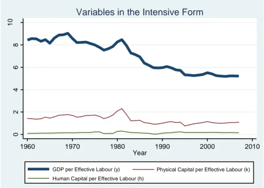
It is possible to observe that Human Capital has not being constant along the time. The investment in this variable had an important decrease at the end of the 1970’s and in the 1980’s. Since 1990, it has been almost constant, but still decreasing. This variable shows us the role of the investment in Education in Mexico, which has been uncertain during the past 47 years. Although today it is still in its highest levels. The variables are transformed in Figure 5-2 in order to work with them as the Solow model indicates. Each original variable was divided by the Effective Labour variable (AL).

In Figure 5-3 the savings in Human Capital (s_h) during the period analyzed. It is possible to see how it has not been constant along the time. Savings in Human Capital decreased significantly at the end of the 1970’s and the 1980’s. Since 1990, untill now, it has been almost constant, but still decreasing. This variable shows us the role of the investment in Education in Mexico, which has been uncertain during the past 47 years. Although today, it is still in its highest levels.

0 2 4 6 8 10 y = Y/ AL 1960 1970 1980 1990 2000 2010 Year

GDP per Effective Labour (y) Physical Capital per Effective Labour (k) Human Capital per Effective Labour (h)

Variables in the Intensive Form

Figure 5-2 Variables per unit of Effective Labour

0 .0 1 .0 2 .0 3 .0 4 Sa vi n g s in H u ma n C a p it a l a s % o f G D P 1960 1970 1980 1990 2000 2010 Year

Savings in Human Capital

The savings in Physical Capital shown in Figure 5-4 are really interesting. First we can observe a clear growth in this variable since 1960 untill the early’s 80’s, but after that episode, the savings in physical capital started to decrease along the time. Also an important decrease can be seen in the 1994 economic crisis.

.5 1 1 .5 2 2 .5 Sa vi n g s in Ph ysi ca l C a p it a l a s % o f G D P 1960 1970 1980 1990 2000 2010 Year

Savings in Physical Capital

Figure 5-4 Savings in Physical Capital from 1960-2007

Each decade has had a different production pattern along the time. This can be examined in Figure 5-5, where it is possible to differentiate between the economy that each decade has had to face. It is important to analyze that during the recent years (2000-2007) the variables have been stable. This is due to to macroeconomic policy followed by the Mexican Government.

The next Tables (5-1 & 5-2) show the results of the estimated model for the analyzed pe-riods:

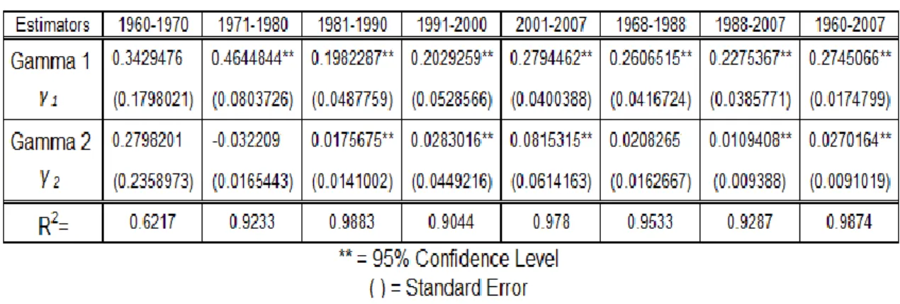
Table 5-1 Results of the Estimated Regressions for each period

Table 5-2 Results of the Original Parameters of the Production Function

It is important to illustrate that for the 1970s and 1980s, as well as for the period 1968-1988, the estimators Gamma 2 (γ₂) were not statistically significant at a 95% confidence level. So it is possible to see that human capital was not a significant source of growth dur-ing those decades in Mexico.

The estimation was done for different periods in order to analyze with more efficiency the variables involved in the Solow model. First it was done for each decade since 1960 until 2007 and after that for two crucial periods in the economic history of Mexico. The first one runs from 1968 to 1988, which is marked by a significant economical intervention of the state in the economy and the second one, from 1988 until 2007, characterized by a neoli-beral state, concerned about the macroeconomic stability and the market efficiency. The last regression was done for the entire period analyzed (1960-2007).

The R-Squared of the period 1960-1970 is low compared to the rest in the other periods analyzed. The explication for this is that the model is not very adjusted to this period. Ac-tually, neither the variable lns_h was statistically significant at a 95% confidence level, nor lns_k. Although this las one was statistically significant at a 94.4% confidence level.

The results of the regressions and the autocorrelation tests (Durbin Watson Statistic and Breusch- Godfrey LM test for autocorrelation) are all presented for each period analyzed in the Appendices. For more information regarding the fundamentals and functions of the tests is suggested for the reader to check Gujarati (2004) and Greene (2008).

5.1 Growth Accounting

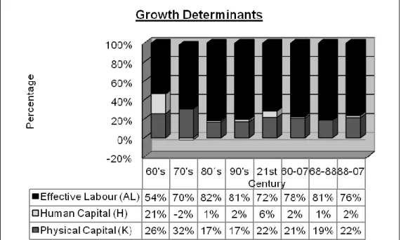
The model yields interesting results, in which it is possible to observe the composition of the production factors in general and for periods. For the analysis of 1960-2007 as a whole, we can observe that Mexico is a country based on the workforce.

The strongest factor of creation of growth in Mexico over the past 47 years has been the Effective Labor, with approximately 76.34%. In second place, the Physical Capital with 21.54% and in last place the Human Capital with only 2.12%.

However, it is important to note that the decade that witnessed one of the greatest eco-nomic growth in the history of Mexico (1960), the contribution of Human Capital played a more predominant role in the development of the economy, with 20.84% while the Capital 25.54% and 53.63% the Effective Labour.

Mexico experienced a higher economic growth in that time period thanks to the larger pro-portion on savings of Physical Capital (sk) and Human Capital (sh). This can be appre-ciated on Figure 5-6.

Figure 5-6 Growth Contribution by Economic Factor and Period analyzed

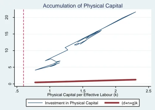
The Solow model (1956) indicates that the higher the saving rate is, the higher steady state of long term and in consequence, a higher level of capital stock per Effective Labour (k* & h*).

Figures 5-7 and 5-8 show the steady state to which the Solow Model tends. The long run equilibriums, according to the model, are given by the intersection of the investment in

Physical or Human Capital with the identities of (δ+n+g)k or (δ+n+g)h respectively. It is observed that both equilibriums for Mexico are low; especially for Human Capital. This two figures represent the steady state of the Solow Model and are analogous to Figure 3-1. It is possible to observe also that although the Physical Capital has increased considerably in the 70's, this investment was made mostly by the Mexican Government and not by pri-vate capital. So its performance was not as productive, as what the pripri-vate capital would have been able to create.

0 5 10 15 20 G D P p e r Ef fe ct ive L a b o u r (y) .5 1 1.5 2 2.5

Physical Capital per Effective Labour (k)

Investment in Physical Capital (d+n+g)k

Accumulation of Physical Capital

Figure 5-7 Steady State and Accumulation of the Physical Capital

0 .1 .2 .3 G D P p e r Ef fe ct ive L a b o u r (y) 0 .02 .1 .2 .3

Human Capital per Eeffective Labour (h)

Investment in Human Capital (d+n+g)h

Accumulation of Human Capital

During the 1980s Mexico experienced a Structural Adjustment and since this time the sav-ings in physical capital have tended to increase in a moderate way, due to the levels of For-eign Direct Investment in the country which have tended to rise.

However, the model yields interesting results, in which can be observed that only in the present decade savings in physical capital have a weight of 21.84%. But even without reach-ing the levels of the 1960’s (25.54%) or even the ones of the 1970’s (31.72%) which have been the highest in all the periods analyzed. Also the investment in human capital has in-creased during this decade and is now at levels of 6.37%, however still below the levels of the 1960’s (20.84%).

It is important to say that the model reflects the actual effort of the country to invest in Human Capital, Education, achieving the highest levels in years. It is the first time that this variable, as a proportion of the GDP, is higher than the average of educational investment of the OECD countries (4%). A major dilemma within this investment is that a 97.2% is current expenditure and not investment directly in Human Capital. Actually, 93.6% of the current expenditure corresponds only to wages (Granados, 2005).

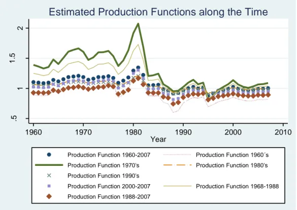
The following graph (Figure 5-9) is very interesting, because time is graphed against the various functions of production estimated for each period. So, it is possible to observe the growth that was experienced in each point of time with each estimated function. It is re-markable that today the production function that would generate higher economic growth in Mexico would be the one of the 70's, because that function is composed of 31.72% of investment in physical capital. However, such investment should be done by private capital to generate real economic growth and not by the government as it was held during that time. .5 1 1 .5 2 G D P p e r Ef fe ct ive L a b o u r [f (k, h )] 1960 1970 1980 1990 2000 2010 Year

Production Function 1960-2007 Production Function 1960´s Production Function 1970's Production Function 1980's Production Function 1990's

Production Function 2000-2007 Production Function 1968-1988 Production Function 1988-2007

Estimated Production Functions along the Time

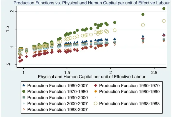
Moreover, Figure 5-10 shows that the current production function is generating an eco-nomic growth that roughly conforms to the average of all production functions studied. It is for this reason it is important that Mexico generate and apply policies that at some point worked in the past years and contribute to a real and sustained growth of the economy.

.5 1 1 .5 2 G D P p e r u n it o f Ef fe ct ive L a b o u r [f [k, h ] 1 1.5 2 2.5

Physical and Human Capital per unit of Effective Labour Production Function 1960-2007 Production Function 1960-1970 Production Function 1970-1980 Production Function 1980-1990 Production Function 1990-2000

Production Function 2000-2007 Production Function 1968-1988 Production Function 1988-2007

Production Functions vs. Physical and Human Capital per unit of Effective Labour

Figure 5-10 Estimated Production Functions compared to the levels of Physical and Human Capital in the Intensive Form

6

Conclusions

Mexico is a country in which citizens, entrepreneurs and government must work hard to solve issues of great impact. First, it is clearly showed by this model, the huge backward-ness currently experienced in the field of investment. Private and foreign investment in Mexico has not grown significantly. It is important that the State assume its responsibility and generate the legal framework under which, it could be possible to attract more invest-ment to the country.

The last government (Vicente Fox; 2000-2006) was characterized by a low budget deficit. However, it is now clear that there is no question of falling into a populist government like in the 70's to be able to invest, but is simply a matter that governments should spend public resources responsibly in sources that generate sustainable growth.

Nowadays the President of Mexico Felipe Calderón launched the National Infrastructure Program. In this program, the government will invest millions of Mexican Pesos on high-ways, roads, bridges and physical infrastructure. This will facilitate an efficient transporta-tion of materials, goods and people. Moreover this will reduce the cost and time in which incurs the economy and increase the productivity of the country.

The current financial crisis is affecting almost every country in the world, and Mexico is not excluded from its impacts. Moreover, Mexico will face serious problems during 2009 in terms of economic growth. It is for this reason why the “visible hand” of the State would be required in order to invest in sources that generate growth and development. The model verified that the higher the rate of investment in Physical and Human Capital, the higher the steady state of equilibrium in the long run. For this reason it is extremely important the National Infrastructure Program as a source of growth and tool against the actual world fi-nancial crisis.

The Government is planning to invest 6% of the GDP in the next year on this Pro-gram(Presidencia de la República, 2008) and according to the model exposed; this will con-tribute with 28% of the investment on Physical Capital in 2009, which would generate a 1.5% of growth of the GDP in 2009.

In second place, the government should focus on attracting greater foreign investment, es-tablishing a legal framework, efficient and competitive in which all agents can interact free-ly. Several studies in terms of competitiveness (Ros; 2004 & Bonnefoy, et al; 2005) have re-vealed that Mexico has three types of setbacks:

 Competitiveness on Currency Exchange  Institutional Development

 Business Environment

National Transparency, a company dedicated to lifting surveys on corruption in Mexico since 2001, published in 2007, the Index of Corruption and Good Governance, which found that only in 2007 there were 197 million acts of corruption and bites totaled $ 27 bil-lion pesos (more than 2 Bilbil-lions of USD). The Mexican households spend on average per year between 8% and 18% of their income for these illegal purposes (National Transparen-cy, 2008).

Several studies have analyzed the impact of corruption on economic growth and according to the study of Mauro (1995), an improvement of one standard deviation in the index of corruption is associated with an increased rate of investment in 2.9% of GDP.

Finally, investment in education is a major source of economic growth and economic de-velopment; moreover it improves the living standards considerably. The developed coun-tries invest in Research and Development (R & D) between 1.5% and 2% of its GDP, while Mexico has been investing throughout these years in R & D, only 0.34% of its GDP. On education, Mexico has during the last years annually invested about 4% of GDP (OECD, 2008). The major problem, as exposed previously, is that 97.2% of this invest-ment is in current expenditure and not directly in Human Capital.

It is for this reason that Mexico needs to increase its productive investments in Human Capital, like for example, in more schools, new program studies, Research & Development, scholarships, etc. In the last educational evaluation, PISA, made by the OECD (2008) to the members of this organization, Mexico got the last place. The sole investment in educa-tion does not guarantee that the Human Capital will achieve higher levels of productivity. That is why it is important to improve and extend the savings’ plans on this field.

The exogenous growth Solow model is easy to understand and is well suited to the charac-teristics of any country. With this model becomes much simpler the modeling and quantifi-cation of the determinants of economic growth.

In the case of Mexico, this model found that the determinant of growth during the periods analyzed is mostly conformed by Effective Labour (76.34%), rather than Human Capital (2.12%) or Physical Capital (21.54%). Although for certain periods analyzed, like the dec-ade of 1960’s the Human Capital played an important role in the economic growth of the country with 20.84%.

The results of the regressions, for each period, showed that in general the investments in human and physical capital are low. The highest investment in Physical Capital was done in the 1970’s with 31.72%, which is still a low parameter compared to industrialized and de-veloped countries like United States or Sweden. The results within the parameter of Hu-man Capital were a little bit complicated, because for the periods of 1970’s, 1980’s and 1968-1988, the value of this parameter was not significant. This means that the Human Capital was not a determinant of growth for Mexico’s economy during this periods.

The regressions for the periods of 1968-1988 and 1988-2007 showed a small difference in the composition of the determinants of growth in Mexico. For the first period mention, the Physical and Human Capital is higher than in the second period analyzed. The only differ-ence is within the Effective Labour which became stronger in the second period (80.57%) than in the first one (77.67%). All this results are supported by the economic backgrounds and policies of each period analyzed

It is important to mention that also the model revealed that the economic policies followed by the government during the period 1968-1988 generated the highest economic growth. However, this investment was not as productive as it should have been if it was done by the private sectors of the country. For this reason is also important to make a distinction between the public and private investment in the Augmented Solow Model for further ana-lyses.

The contribution of this thesis is that there are few papers that apply econometrics within an Augmented Solow Model and specially to analyze the case of a single country, in this case Mexico. Most of the papers only apply dynamic macroeconomics with phase diagrams or calibration processes in order to have the parameters of Solow.

The results of this paper correspond with the theory and background of Mexico. For this reason the Aumented Solow Model gives a clear scenario of what have been Mexico’s economy and is well suited for further analyses.

6.1 Suggestions for Further Research

The studies and advances in Exogenous Growth theory are increasing by the years. There are studies that differ in the assumptions of the model. These can be applied to measure the determinants of the economic growth. First of all, it would be interesting for Mexico’s analysis to apply the model under the assumptions of imperfect competition (instead of perfect competition) and/or increasing returns to scale. This type of model will give a more real scenario in order to study the case of Mexico.

Also, what can be done is to make a panel analysis for Mexico, but within the different sec-tors in the economy. With this type of model the results would be more precise, showing which sectors are contributing more to Mexico’s growth. In consequence, it would be easi-er to give information about the industries in which is missing investment or savings in or-der to achieve higher levels of growth and development.

References

Electronic Sites:

World Bank. World Development Indicators. Recovered from the WEB the 21st of April 2008 from: www.worldbank.org

Banxico. Publicaciones. Recovered from the WEB the 25th of April 2008 from: www.banxico.gob.mx

International Monetary Fund. International Financial Statistics. Recovered from the WEB the 21st of April 2008 from: www.imf.org.

INEGI. National Accounts. Recovered from the WEB the 25th of April 2008 from: www.inegi.gob.mx

OECD. National Accounts of OECD. Recovered from the WEB the 28th of April 2008 from: http://www.oecd.org/topicstatsportal/0,3398,en_2825_495684_1_1_1_1_1,00.html Presidencia de la República. National Infrastructure Program 2007-20012. Recovered from the

WEB the 28th of November 2008 from:

http://www.infraestructura.gob.mx/index.php?page=english-version

National Transparency. ICBG. Recovered from the WEB the 3rd of May 2008 from: www.transparenciamexicana.org.mx

Books:

Agudelo, Mercedes (1997). Ajuste estructural y pobreza. México: ITESM-FCE. Capítulo V, "El ajuste estructural en México y sus implicaciones económicas", pp. 335-363.

Aspe, P. (1993). El Camino mexicano de la transformación económica. Fondo de Cultura Econó-mica: México, D.F

Greene, W. (2008). Econometric Analysis.Prentice-Hall Pearson: Upper Saddle, N.J. Gujarati, D. (2004). Econometría. Mc-Graw Hill: Mexico

INEGI. (2001). El Ingreso y el Gasto Público en México. INEGI: México D.F.

INEGI. (2007). Agenda Estadística de los Estados Unidos Mexicanos. INEGI: México D.F. Krauze, Enrique. La Presidencia Imperial. Ascenso y caída del sistema político

mexica-no(1940-1996). Ed. Tusquets, México, 1997

Nacional Financiera. (1990). La economía mexicana en cifras 1990. Publicaciones: México D.F. Nacional Financiera. (1998). La economía mexicana en cifras 1998. Publicaciones: México D.F. Romer, D. (2006) Macroeconomía Avanzada, McGraw-Hill, México, D.F.

Journals:

Bonnefoy, J.; Armijo, M. (2005). Indicadores de desempeño en el sector público. Series Manuales, CEPAL: Santiago de Chile

Granados, Otto (2005). Educación en México ¿Gastar más o invertir mejor? Observatorio Ciudadano de la Educación. Vol. V, No. 148: México

Heston, A.; Summers, R. & Aten, B. Penn World Table Version 6.2, Center for International Comparisons of Production, Income and Prices at the University of Pennsylvania, September 2006.

Lucas, Robert E. Jr. (1988). “On the mechanics of development planning”. Journal of Monetary Ecnomics, 22(1), July.

Mankiw, N.G., Romer, D., y Weil, D.N. (1992). A contribution to the Empirics of the Economic

Growth, Quarterly Journal of Economics, 107, 407-37

Mauro, Paulo. (1995). Corruption and Growth. Quarterly Journal of Economcs, 110 (3), pags. 681-713.

Romer, Paul. (1986). “Increasing returns and long-run growth”, Journal of Political Economy, 94(5), October.

Ros, J. (May 2004). El crecimiento económico en México y Centroamérica: desempeño reciente y

perspecti-vas. Series de Estudios y Perspectivas, CEPAL: México, D.F.

Solow, RM. (1956). A contribution to the theory of economic growth. Quarterly Journal of Eco-nomics. 70: 65-94

Temple, Jonathan (January, 1998). Equipment investment and the Solow model. Oxford Econom-ic Papers; 50, 1; ABI/INFORM Global pg. 39

Appendices

Appendix 1:

Source | SS df MS Number of obs = 11 ---+--- F( 3, 7) = 3.84 Model | .005715196 3 .001905065 Prob > F = 0.0650 Residual | .003476946 7 .000496707 R-squared = 0.6217 ---+--- Adj R-squared = 0.4596 Total | .009192142 10 .000919214 Root MSE = .02229 --- ln(y) | Coef. Std. Err. t P>|t| [95% Conf. Interval] ---+--- ln(sk) | .410919 .1798021 2.29 0.056 -.0142454 .8360835 ln(sh) | -.0016252 .2358973 -0.01 0.995 -.5594337 .5561833 t | -.0065276 .0133173 -0.49 0.639 -.0380179 .0249627 _cons | 1.999106 1.05311 1.90 0.099 -.4911043 4.489316 --- . Durbin Watson Statistic: Durbin-Watson d-statistic( 4, 11) = 1.581496 . Breusch-Godfrey LM test for autocorrelation

--- lags(p) | chi2 df Prob > chi2 ---+--- 1 | 0.106 1 0.7449 2 | 3.112 2 0.2110 3 | 4.275 3 0.2333 4 | 8.209 4 0.0842 5 | 8.548 5 0.1285 6 | 11.000 6 0.0884 --- H0: no serial correlation

Appendix 2:

Source | SS df MS Number of obs = 11 ---+--- F( 3, 7) = 28.10 Model | .013995065 3 .004665022 Prob > F = 0.0003 Residual | .001162184 7 .000166026 R-squared = 0.9233 ---+--- Adj R-squared = 0.8905 Total | .015157249 10 .001515725 Root MSE = .01289 --- ln(y) | Coef. Std. Err. t P>|t| [95% Conf. Interval] ---+--- ln(sk) | .4575577 .0803726 5.69 0.001 .2675067 .6476088 ln(sh) | -.0331857 .0165443 -2.01 0.550 -.0723067 .0059353 t | -.0167452 .0021778 -7.69 0.000 -.0218948 -.0115956 _cons | 1.931229 .0850877 22.70 0.000 1.730028 2.132429 --- . Durbin Watson Statistic:

Durbin-Watson d-statistic( 4, 11) = 1.65009 . Breusch-Godfrey LM test for autocorrelation

--- lags(p) | chi2 df Prob > chi2 ---+--- 1 | 1.872 1 0.1712 2 | 3.311 2 0.1910 3 | 4.377 3 0.2236 4 | 6.143 4 0.1887 5 | 8.428 5 0.1342 6 | 10.247 6 0.1146 --- H0: no serial correlation

Appendix 3:

Source | SS df MS Number of obs = 11 ---+--- F( 3, 7) = 197.46 Model | .179195944 3 .059731981 Prob > F = 0.0000 Residual | .002117485 7 .000302498 R-squared = 0.9883 ---+--- Adj R-squared = 0.9833 Total | .181313429 10 .018131343 Root MSE = .01739 --- ln(y) | Coef. Std. Err. t P>|t| [95% Conf. Interval] ---+--- ln(sk) | .2033323 .0487759 4.17 0.004 .0879956 .3186691 ln(sh) | .0165125 .0141002 1.17 0.280 -.0168292 .0498543 t | -.0213402 .0040223 -5.31 0.001 -.0308515 -.011829 _cons | 2.463143 .1294826 19.02 0.000 2.156966 2.769321 --- . Durbin Watson Statistic:

Durbin-Watson d-statistic( 4, 11) = 1.45785 . Breusch-Godfrey LM test for autocorrelation

--- lags(p) | chi2 df Prob > chi2 ---+--- 1 | 1.498 1 0.2210 2 | 2.310 2 0.3151 3 | 2.930 3 0.4026 4 | 4.189 4 0.3810 5 | 8.601 5 0.1261 6 | 10.217 6 0.1158 --- H0: no serial correlation

Appendix 4:

Source | SS df MS Number of obs = 11 ---+--- F( 3, 7) = 22.09 Model | .027295069 3 .009098356 Prob > F = 0.0006 Residual | .002883691 7 .000411956 R-squared = 0.9044 ---+--- Adj R-squared = 0.8635 Total | .03017876 10 .003017876 Root MSE = .0203 --- ln(y) | Coef. Std. Err. t P>|t| [95% Conf. Interval] ---+--- ln(sk) | .2020995 .0528566 3.82 0.007 .0771136 .3270855 ln(sh) | .0152119 .0449216 0.34 0.074 -.0910107 .1214345 t | -.0116201 .0024658 -4.71 0.002 -.0174508 -.0057894 _cons | 2.183996 .2183942 10.00 0.000 1.667576 2.700417 --- . Durbin Watson Statistic:

Durbin-Watson d-statistic( 4, 11) = 1.642179 . Breusch-Godfrey LM test for autocorrelation

--- lags(p) | chi2 df Prob > chi2 ---+--- 1 | 0.008 1 0.9280 2 | 1.822 2 0.4022 3 | 6.304 3 0.0977 4 | 7.555 4 0.1093 5 | 9.321 5 0.0969 6 | 10.488 6 0.1056 --- H0: no serial correlation

Appendix 5:

Source | SS df MS Number of obs = 8 ---+--- F( 3, 4) = 59.40 Model | .003333637 3 .001111212 Prob > F = 0.0009 Residual | .000074829 4 .000018707 R-squared = 0.9780 ---+--- Adj R-squared = 0.9616 Total | .003408467 7 .000486924 Root MSE = .00433 --- ln(y) | Coef. Std. Err. t P>|t| [95% Conf. Interval] ---+--- ln(sk) | .3003008 .0400388 7.50 0.002 .1891354 .4114663 ln(sh) | .0747304 .0614163 1.22 0.029 -.0957886 .2452493 t | -.0063912 .0009496 -6.73 0.003 -.0090277 -.0037548 _cons | 2.186045 .1819313 12.02 0.000 1.680923 2.691167 --- . Durbin Watson Statistic:

Durbin-Watson d-statistic( 4, 8) = 2.215558 . Breusch-Godfrey LM test for autocorrelation

--- lags(p) | chi2 df Prob > chi2 ---+--- 1 | 3.259 1 0.0710 2 | 4.984 2 0.0827 3 | 5.805 3 0.1215 4 | 8.000 4 0.0916 5 | 8.000 5 0.1562 6 | 8.000 6 0.2381 --- H0: no serial correlation

Appendix 6:

Source | SS df MS Number of obs = 21 ---+--- F( 3, 17) = 116.31 Model | .247630465 3 .082543488 Prob > F = 0.0000 Residual | .012064689 17 .000709688 R-squared = 0.9535 ---+--- Adj R-squared = 0.9453 Total | .259695154 20 .012984758 Root MSE = .02664 --- ln(y) | Coef. Std. Err. t P>|t| [95% Conf. Interval] ---+--- ln(sk) | .2606518 .0416724 6.25 0.000 .1727307 .3485728 ln(sh) | .0208265 .0162667 1.28 0.218 -.0134932 .0551462 t | -.0118939 .0010832 -10.98 0.000 -.0141793 -.0096085 _cons | 2.206176 .0880189 25.06 0.000 2.020473 2.39188 --- . Durbin Watson Statistic:

Durbin-Watson d-statistic( 4, 21) = 1.5334459 . Breusch-Godfrey LM test for autocorrelation

--- lags(p) | chi2 df Prob > chi2 ---+--- 1 | 12.116 1 0.0005 2 | 12.538 2 0.0019 3 | 12.585 3 0.0056 4 | 12.593 4 0.0134 5 | 14.449 5 0.0130 6 | 15.043 6 0.0199 --- H0: no serial correlation

Appendix 7:

Source | SS df MS Number of obs = 20 ---+--- F( 3, 16) = 69.50 Model | .057569735 3 .019189912 Prob > F = 0.0000 Residual | .004418053 16 .000276128 R-squared = 0.9287 ---+--- Adj R-squared = 0.9154 Total | .061987789 19 .003262515 Root MSE = .01662

--- ln(y) | Coef. Std. Err. t P>|t| [95% Conf. Interval] ---+--- ln(sk) | .2278065 .0385771 5.91 0.000 .1460267 .3095863 ln(sh) | .0096652 .009388 1.03 0.031 -.0102364 .0295668 t | -.0080622 .0007976 -10.11 0.000 -.009753 -.0063715 _cons | 2.037935 .0568387 35.85 0.000 1.917443 2.158428 --- . Durbin Watson Statistic:

Durbin-Watson d-statistic( 4, 20) = 1.285483 . Breusch-Godfrey LM test for autocorrelation

--- lags(p) | chi2 df Prob > chi2 ---+--- 1 | 2.467 1 0.1162 2 | 2.937 2 0.2302 3 | 3.065 3 0.3817 4 | 3.109 4 0.5398 5 | 4.342 5 0.5013 6 | 5.364 6 0.4981 --- H0: no serial correlation

Appendix 8:

Source | SS df MS Number of obs = 48 ---+--- F( 3, 44) = 1145.51 Model | 1.90328422 3 .634428075 Prob > F = 0.0000 Residual | .02436899 44 .000553841 R-squared = 0.9874 ---+--- Adj R-squared = 0.9865 Total | 1.92765321 47 .041013898 Root MSE = .02353 --- ln(y) | Coef. Std. Err. t P>|t| [95% Conf. Interval] ---+--- ln(sk) | .2836498 .0174799 16.23 0.000 .2484214 .3188782 ln(sh) | .0242075 .0091019 2.66 0.011 .0058638 .0425513 t | -.010341 .0004108 -25.17 0.000 -.0111688 -.0095132 _cons | 2.176481 .0441109 49.34 0.000 2.087581 2.265381 --- . Durbin Watson Statistic:

Durbin-Watson d-statistic( 4, 48) = 1.8376478 . Breusch-Godfrey LM test for autocorrelation

--- lags(p) | chi2 df Prob > chi2 ---+--- 1 | 15.305 1 0.0001 2 | 15.650 2 0.0004 3 | 15.682 3 0.0013 4 | 15.784 4 0.0033 5 | 16.970 5 0.0046 6 | 18.137 6 0.0059 --- H0: no serial correlation

Appendix 9:

Source | SS df MS Number of obs = 48 ---+--- F( 1, 46) = 2597.72 Model | 4.06826372 1 4.06826372 Prob > F = 0.0000 Residual | .072040064 46 .001566088 R-squared = 0.9826 ---+--- Adj R-squared = 0.9822 Total | 4.14030378 47 .08809157 Root MSE = .03957

--- ln A | Coef. Std. Err. t P>|t| [95% Conf. Interval] ---+--- t | .0210149 .0004123 50.97 0.000 .020185 .0218449 _cons | 1.193438 .0116048 102.84 0.000 1.170079 1.216797 ---

Appendix 10:

Source | SS df MS Number of obs = 48 ---+--- F( 1, 46) = 2085.88 Model | 10.5457644 1 10.5457644 Prob > F = 0.0000 Residual | .232565756 46 .005055777 R-squared = 0.9784 ---+--- Adj R-squared = 0.9780 Total | 10.7783302 47 .229326174 Root MSE = .0711

--- ln L | Coef. Std. Err. t P>|t| [95% Conf. Interval] ---+--- t | .0338347 .0007408 45.67 0.000 .0323435 .0353259 _cons | 16.08656 .0208509 771.50 0.000 16.04459 16.12853