SKI Report 2005:36
Research
Reports within the Area of Nuclear Power
Plant Instrumentation
Part 1: Laboratory Test of Analogue and Digital
Instrument Components
Part 2: Dynamic Deviations in Reactor Pressure and
Water Level Signals Caused by Sensing Lines
Bengt-Göran Bergdahl
November 2004
ISSN 1104–1374 ISRN SKI-R-05/36SE
SKI Perspective
Background
This is an English version of the report ”Rapporter inom området sensorteknik, SKI Rapport 2003:07”.
Purpose
The purpose of this English version of the report is to spread the results of the report to a wider audience.
Results
The report discusses dynamic behaviour of instrument components and sensing lines in the light of a couple of different experiments performed either at an actual power plant or in laboratory. These experiments have contributed to SKIs supervision concerning instrumentation issues.
The experiments show, for example, that an analogue density converter is faster than a new digital one. It is also shown that signal analysis is a valuable tool when it comes to detecting unwanted filtering of signals.
The conclusion drawn is that to assure that an important measurement signal is reflecting the physical variable in question in a satisfactory way some kind of dynamic tests are needed. The static calibration is not sufficient, since it will not detect unwanted filtering and a prolonged response time.
Project information
SKI reference: 14.05-011184-01279 (the Swedish version)
Responsible at SKI has been: Kristina Johansson (for the English version) and Annelie Bergman (for the Swedish version).
SKI Report 2005:36
Research
Reports within the Area of Nuclear Power
Plant Instrumentation
Part 1: Laboratory Test of Analogue and Digital
Instrument Components
Bengt-Göran Bergdahl
GSE Power Systems AB
Box 62
611 22 Nyköping
November 2004
SKI Project Number XXXXX
This report concerns a study which has been conducted for the Swedish Nuclear Power Inspectorate (SKI). The conclusions and viewpoints presented in the report are those of the author/authors and do not necessarily coincide with those of the SKI.
Abstract
Reliable measurement signals are of great importance for the safety of a nuclear power plant. The measurement signals are used as input signals to the automatic control systems, they have influence on the reactor protection system and they are the input to the information presented in the control room. Measurement signals are also the basis for analysis of sampled signals after an event. These facts imply that it is important that the measurement data represent physical magnitudes in a correct manner. This holds true both for the static and the dynamic part of the signal.
Mainly depending on the fact that the Swedish BWRs were constructed in the seventies and eighties, the instrument systems were originally designed with analogue technique. This is valid for transmitters as well as density converters, isolation amplifiers and controllers. Right now there is an ongoing modernization of the instrument systems in many plants. Old analogue components are in many cases replaced by new digital ones. The delay time is the critical dynamic deviation between an analogue and a digital transmitter. A delay time of up to 200 ms has been observed for a digital transmitter (Hartmann & Braun ASK800) in comparison with an analogue one (Fujii). A long delay time is of course undesirable when the transmitter is a part of the reactor protection system. It is therefore important to pay attention to the delay in response when an analogue transmitter is replaced by a digital one. The laboratory tests also included a comparison between an old analogue density converter (Hartmann & Braun TZA2) and a new digital one (Hartmann & Braun TZA4). These results prove that the analogue unit is faster than the digital. The response time from differential pressure to level signal was 50 ms for TZA2 and 250 ms for TZA4. Corresponding times with pressure as input and level as output was 50 ms for TZA2 and 900 ms for TZA4.
The report also includes an investigation of pressure transmitters of the type TDE220. The transmitters exhibited deviating dynamics during ordinary sensor tests. The laboratory test confirms the observed deviation in comparison with transmitters of other types. The construction with Bourdon tube is judged to be the reason for the deviations. The report also presents results from trouble shooting with steam pressure transmitters at KKM (Kernkraftwerk Mühleberg in Switzerland). It was possible to identify the intermittent sensor error with the aid of controlled pressure changes. Service of the transmitter pointed out a crack on the electronic filter unit. This was judged to be the reason for the intermittent signal interrupts.
Finally, two possibilities used at KKM to investigate the dynamics of temperature sensors are described. Both methods are based on artificial cooling of the sensor. One of them is applied during power operation of the plant and the other during outage.
Table of contents
1 Background 7
1.1 Reactor water level measurement in a BWR 8
1.2 Analogue and digital instrument components 8
1.3 The content of the report 8
2 Exchange of analogue to digital instrument components 9 2.1 Comparison between an analogue and a digital transmitter at Oskarshamn 2 9 2.2 Comparison between two digital and one analogue transmitter at Ringhals 1 10 2.3 A comparison between an analogue and a digital density converter 16 2.4 Replacement of all instrument components in the water level measurement 17 3 Laboratory investigation of pressure transmitters with Bourdon tube design 21 4 Experiments with an error indicated steam pressure sensor 24
4.1 Steam pressure transmitter MP05B2 24
4.2 Exchange of the transmitter MP05B2 26
5 Methods of investigating temperature sensors 28
5.1 Investigation of air temperature 28
5.2 Investigation of the temperature sensors in torus 28
6 Conclusions 33
1 Background
Reliable measurement signals are of great importance for the safety of a nuclear power plant. The measurement signals are used as input signals to the automatic control systems, they have influence on the reactor protection system and they are the input to the information presented in the control room. Measurement signals are also the basis for analysis of sampled signals after an event. These facts imply that it is in important that measurements represent physical magnitudes in a correct manner. This holds true for both the static and the dynamic part of the signal.
The measurement systems consist of many instrument components connected in cascade. For the measurement of e.g. water level in a BWR there are sensing lines, transmitters for differential and reactor pressure, and a density converter. See figure 1.1. Further instrument components like isolation amplifiers can exist in the instrument system in cascade thereafter.
To guarantee good static performance, annular calibration of the transmitters is performed at the plant. Observed static deviation is corrected in connection to these routines. In this way it is secured that the measurement systems have acceptable accuracy in their static presentation.
The dynamic character of the measurement system components is seldom or never tested in BWRs. This implies that transients in the plant may be filtered away in the measurement systems and therefore not be observed. Unwanted filtering of the measurement signals may also give rise to delayed reaction of the protection system during a transient.
Figure 1.1 Measurement system for the water level in a boiling water reactor.
Reactor vessel
Pressure transmitter
DP transmitter Density
converter Isolation amplifier Condensate pot
Sensing line
Electronic signal (0-10) V or (0-20) mA
1.1 Reactor water level measurement in a BWR
Figure 1.1 is a block diagram for a reactor water level measurement system. The differential pressure transmitter (blue) is connected to pressure taps on the reactor vessel with two sensing lines. The electronic output from the transmitter is proportional to the difference between the condensate pot level and reactor water level. This is the DP-signal and at the same time one of the inputs to the density compensation units (yellow). The density compensation unit has the differential pressure, DP, and reactor pressure, P, as inputs and the density compensated water level signal as output. After the density compensation unit isolation amplifiers follows; see Figure 1.1.
1.2 Analogue and digital instrument components
Mainly depending on the fact that the Swedish BWRs were constructed in the seventies and eighties, the instrument systems were originally designed with analogue technique. The components in question are transmitters, density converters, isolation amplifiers and regulators. Now when the instrument systems are modernized in many plants they are replaced by newly developed units. This often implies that old analogue components are replaced by digital ones.
It is important to consider reliability, expected lifetime, capability of resisting temperature and radiation and so on when instrument components are exchanged. It is also, however, important that the response time of the new component is acceptable.
1.3 The content of the report
This report presents results from sensor investigations with instrument components. The thing in common for most of the experiments are that the components have been tested in a laboratory environment or under such operational conditions that accepted experiments. The investigations include:
• A comparison between analogue and digital transmitters and density converters. • A comparison between analogue pressure transmitters of different designs. • Operational experience with a not correct working pressure transmitter and the
experiment to identify the fault.
• A description of methods for testing temperature sensors when they are already installed in the plant.
2 Exchange of analogue to digital instrument
components
There is an interesting development in process industry when we talk about instrumentation and surveillance. The trend is that old analogue instrument components are replaced by new digital ones. This is the case for e.g. digital transmitters and digital controllers. Added to that, the field-bus has been available in process industry for many years. With the aid of a field-bus all transmitters in a plant can be connected in a network, and from a central place in the plant an arbitrary transmitter can be addressed for adjustment of e.g. physical range.
It will take a long time before field-busses are introduced at a grander scale in nuclear power plants. The reason for this is of course the special quality demands in the nuclear industry. On the other hand, digital controllers, transmitters and other digital components are already in use in nuclear power plants. The transfer to digital instrument components happens gradually. Old analogue units, not any longer in storage, are replaced by modern digital components. Typical is that the analogue input-output standard (e.g. 4-20 mA) still is valid. A digital transmitter has for example an analogue output. The same thing holds true when controllers are replaced. There are often analogue inputs and outputs. There are also examples where internal controller signals are D/A-converted to correspond to measurement possibilities that were available in the old analogue controller.
The present chapter compiles some results from different measurement campaigns performed by GSE Power Systems AB. The main focus in the presentation is the dynamic character of the components. The comparison between analogue and digital components presented in this report is performed with the individual parameter adjustment that was valid for the component. The report does not discuss the possible filtering of each component.
2.1 Comparison between an analogue and a digital transmitter at
Oskarshamn 2
At a sensor investigation at Oskarshamn 2 in 1997 a comparison was carried out between an analogue and a digital pressure transmitter. The comparison was performed in a laboratory where the transmitters were exposed to a common fast fluctuating pressure at the same time as their output signals were recorded; see Figure 2.1. For practical reasons pneumatic air was used as the pressure source. This fact limited to some extent the rapidity of the pressure changes.
The transmitter signals for the complete experiment from the analogue transmitter Fujii and the digital transmitter ASK800 are displayed in Figure 2.2. In this time scale the figure confirms that there is good agreement between both signals. A closer examination of the signals in an expanded time scale proves the dynamic deviation between the transmitters; see Figure 2.3. The digital transmitter ASK800 reacts with a delay time in relation to the analogue transmitter Fujii during the pressure reduction displayed in Figure 2.3.
Figure 2.4 explains the parameters that will be used to describe the transmitter dynamics. The figure displays a step input signal and corresponding output signal. The output signal reacts with a delay time and a time constant. The delay time (or transport time) is called Td and the time constant Tc. The time constant is defined as the time it takes for the output to grow to 63.2 % of the final value, not taking the delay time into account; see Figure 2.4. The transport time is a pure delay time; that is the time before the component starts to react at all.
From experience we know that analogue components are characterized by a response with a time constant but without a delay time. The digital components on the other hand have a response characterized by a time constant as well as a delay time.
For the digital transmitter ASK800, the delay time was estimated to Td = 200 ms; see Figure 2.3. One can also observe that ASK800 has a longer time constant Tc than Fujii. This is obvious since the slope for Fujii is steeper than corresponding slope for ASK800 during pressure reduction. With the aid of process identification a model has been calculated that describes the relation between the two signals. In this case Fujii is treated as input signal and ASK800 as output signal. A step test of the identified model is presented in Figure 2.5. The results indicates that Td + Tc = 330 ms. Observe that this is the dynamic difference between the two transmitters.
The APSDs (Auto Power Spectral Density) for the signals from the laboratory experiment are presented in Figure 2.6. The figure show that the APSDs agree with each other up to 1 Hz. Thereafter ASK800 is clearly damped in comparison with Fujii. Evidently it is the extra filtering included in ASK800 that causes the observed damping. According to a note from the experiments at Oskarshamn, ASK800 included a filter with the time constant Tc = 0.125 s. This can explain the deviation in slope for the transmitter signals during pressure reduction as it is shown in Figure 2.3.
2.2 Comparison between two digital and one analogue transmitter at
Ringhals 1
An investigation similar to the one described in Chapter 2.1 has been performed at Ringhals 1. This time two digital and one analogue pressure transmitter were studied in laboratory. The transmitters were Hartmann & Braun AVI200, Rosemount 3051C-smart and Hartmann & Braun ASK800. Out of these AVI200 is analogue while the others are digital.
The three transmitters were connected to a common pressure source in a similar way as in the experiments presented in chapter 2.1. Sampling of transmitter signals started during simultaneous variation of pressure. The results of the pressure fluctuations are displayed in Figure 2.8 and 2.9. Qualitatively, this is the same pattern as during the experiments in Oskarshamn. Both of the digital transmitters have a delay time in comparison with the analogue transmitter. The analogue transmitter is therefore faster in the beginning. An estimate of the delay time has been performed and the results are Td = 95 ms for ASK800 and Td = 60 ms for Rosemount 3051C. It is also interesting to note that the transmitter Rosemount 3051C lacks internal filter in this test. This is the reason for the edges on the curve in comparison with the other signals. Another observation is that Rosemount 3051C in spite of a delay time reaches the final value
time constant Tc is shorter for Rosemonut 3051C than for AVI200. It is also obvious that ASK800 has the longest time constant Tc in comparison with the other tested transmitters; see Figure 2.8 and 2.9.
Figure 2.10 shows APSDs for the three transmitter signals. It is clear that the APSDs agree up to 2 Hz, thereafter they disagree. ASK800 has the most damped character above 2 Hz of the three signals. The APSD for AVI200 and Rosemount 3051C agree quite well up to 7-8 Hz. Thereafter the noise content for Rosemount 3051C increases compared to AVI200. This is probably a result of the earlier mentioned edges (high frequency) in the time series data for Rosemount 3051C.
To summarize, it could be said that the critical dynamic deviation between an analogue and a digital transmitter is the delay time. The digital transmitter reacts with a delay time. This can cause trouble when the transmitter is a part of an automatic control system. A delay time in a control loop increases the phase angel and can therefore reduce the stability. A delay time is also annoying when the transmitter is part of the reactor protection system. In this case the triggering of the protection system will be extra delayed with Td for the transmitter. It is therefore important to pay attention to the delay in response when an analogue transmitter is replaced by a digital one.
0 50 100 150 200 250 300 350 -0.5 0 0.5 1 1.5 2
2.5 Time series data for file; O2F97.DAT
Time [sec] Ph ys ic a l U n it ASK-800 fuji
Figure 2.2 Output signals from the transmitters ASK800 and Fujii as a function of time during variation of pressure (P). See also Figure 2.1 above. From Oskarshamn 2, 1997. 0 0.2 0.4 0.6 0.8 1 1.2 1.4 1.6 1.8 2 1.1 1.2 1.3 1.4 1.5 1.6 1.7 1.8 1.9 2
2.1 Time series data for file; O2F97.DAT
Time [sec] Ph ys ic al U n it ASK-800 fuji
Figure 2.3 A closer look at the
difference between the signals from the digital transmitter ASK800 and the analogue transmitter Fujii. The dynamic difference consists of Td = 200 ms and a time constant.
Oskarshamn 2, 1997.
Fujii
ASK 800
Pressure
source
Storage
of data
Delay time TdFigure 2.1 Laboratory test of the digital pressure transmitter ASK 800 in comparison with the analogue transmitter Fujii. Oskarshamn 2, 1997.
Figure 2.4 Definition of delay time Td and time constant Tc. 0 0.5 1 1.5 2 2.5 3 3.5 4 0 0.2 0.4 0.6 0.8
1Open loop step response from fuji to ASK-800; Mo=21 File; O2F97.DAT
Time [sec]
Unit
(MBA
R
)
- Response characteristic parameters
Delay time 0.113(sec) PK overshoot 0.007(%) Time Const. 0.334(sec) Final Value 0.994(MBAR) Rise Time 0.358(sec) Init. Point 100 Settle Time 0.582(sec) No Dt Point 1762 Peak Time 1.181(sec) Sampl. Frq. 53.333(Hz) Peak Value 0.994(MBAR)
Figure 2.5 Step test with the identified model where the signal from Fujii act as input signal and the signal from ASK800 act as output signal. Td + Tc = 0.33 s. Results from Oskarshamn 2, 1997. 10-2 10-1 100 101 102 10-8 10-6 10-4 10-2 100
102 Auto Power Spectra File; O2F97.DAT
Frequency [Hz] A PS D [ (Ph . U n it) ^2 )/ H z] ASK-800 fuji
Figure 2.6 APSD for the ASK800 and Fujii signals based on measurement data from the laboratory experiment at Oskarshamn 2, 1997. Step input 63% 100% Td Tc Time Output
Figure 2.7 Laboratory test of the digital transmitters ASK800 and Rosemount 3051C and the analogue transmitter AVI200. Laboratory investigation performed at Ringhals 1, 2000. 0 0.05 0.1 0.15 0.2 0.25 0.3 0.35 0.4 0.45 0.5 0 0.1 0.2 0.3 0.4 0.5 0.6 0.7 0.8 0.9
Time series data for file; r1lab1.dat
Time [sec] Ph ysi ca l U ni t AVI200 3051Rosemo ASK800
Figure 2.8 Sensor signals from AVI200, Rosemount 3051C and ASK800 during a fast pressure reduction. The digital transmitters displays a delay time. Ringhals 1, 2000. 0 0.1 0.2 0.3 0.4 0.5 0.6 0.7 -0.1 0 0.1 0.2 0.3 0.4 0.5 0.6 0.7 0.8
0.9 Time series data for file; r1lab1.dat
Time [sec] P h ysical Unit AVI200 3051Rosemo ASK800
Figure 2.9 Sensor signals from AVI200, Rosemount 3051C and ASK800 during a fast increase in pressure. The signals from the digital transmitters are clearly delayed. Ringhals 1, 2000.
AVI 200
Rosemount 3051
ASK 800
Pressure
source
Storage
of data
10-2 10-1 100 101 102 10-8 10-6 10-4 10-2 100
102 Auto Power Spectra File; r1lab1.dat
Frequency [Hz] APSD [(Ph. Unit) 2 )/Hz ] AVI200 3051Rosemo ASK800
Figure 2.10 APSD for the sensor signals from AVI200, Rosemount 3051C and ASK800 during experiments with pressure fluctuations. Observe that the APSD functions agree very well up to 2 Hz. Above this frequency there is deviation between the transmitters. Ringhals 1, 2000.
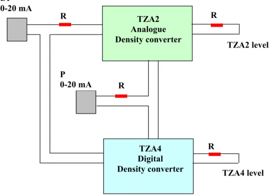
2.3 A comparison between an analogue and a digital density converter
Measurement of the water level in a BWR is performed with differential pressure via the pressure taps on the reactor vessel. As seen in Figure 1.1 the pressure taps are followed by an electronic unit, a so-called density converter. This unit compensates for density. The output signal from the density converter is proportional to the reactor water level. A density converter can have different applications, but it is common in older reactors that the water level is a function of the differential pressure and reactor pressure. This is the case in Figure 1.1. The electronic density converter has differential pressure- and pressure transmitter outputs as inputs and the output from the converter is the reactor water level signal. The density converter is an analogue electronic unit. As was the case with the transmitters, it is now common to replace old analogue converters with digital ones. Such an exchange has been performed at Barsebäck 2 and it is also under way in other plants. Experiments have been performed in laboratory at Barsebäck 2 to investigate the difference in character between an analogue and a digital density converter; see Figure 2.11.
The investigated units are Hartmann & Braun TZA2 (old-analogue) and Hartmann & Braun TZA4 (new-digital). The setup presented in Figure 2.11 will be used, since the converters operate with current signals (0-20 mA). One of the current generators corresponds to DP (Differential Pressure) and the other one to P (Pressure). Observe that the units are connected in such a way that the current signal for DP is equal for both units. The same holds true for signal P. Finally there is a resistance R in all current loops to get voltage to the sampling unit; see Figure 2.11. The current outputs from the converters are equipped with resistors for the same reason.
Figure 2.12 shows the input signal DP and the corresponding level signal TZA2-level from the analogue unit TZA2. The dynamic relation between input and output can be evaluated by identifying the model where DP is input and TZA2-level output. Step test of the model is presented in Figure 2.13. The step test gives that Tc = 50 ms.
The results for the digital density converter TZA4 are displayed in Figure 2.14 and 2.15. The time series data show that the digital density converter has different dynamics. The output signal is clearly delayed compared to the input signal; see Figure 2.14. A model was identified and step tested. The result for the step test in Figure 2.15 is Td + Tc = 250 ms. The time constant and delay time is consequently 5 times longer for TZA4 in comparison with TZA2 regarding the dynamic relation from DP to Level. Figure 2.16 shows the output signals from the density converters TZA2 and TZA4 during variation of the pressure signal P. DP is constant during this experiment. It is obvious that the TZA4-level signal is delayed compared with the TZA2-level signal. Step test of the identified model for the relation between P and TZA4-level is shown in Figure 2.17. The result is that Td + Tc = 934 ms. Corresponding dynamics for the relation between P and TZA2-level is displayed through a step test in Figure 2.18. The figure gives that Tc = 53 ms.
The old analogue unit TZA2 has fast dynamics considering the relation between DP and Level. The same conclusion holds true for the relation between P and Level. Both relations are characterized with Tc = 50 ms. The new digital unit TZA4 is on the other hand clearly slower. The relation between DP and Level is described with
Td + Tc = 250 ms, while the dynamics with P as input and Level as output is described with Td + Tc = 934 ms. The results from the experiments are displayed in Table 2.1.
Table 2.1 Results for the dynamic relation between DP, P and Level for the analogue and digital density converters.
Density converter DP Level P Level
Td + Tc (ms) Td + Tc (ms)
TZA2 (old – analogue) 50 53
TZA4 (new - digital) 250 934
2.4 Replacement of all instrument components in the water level
measurement
Figure 2.19 displays a block diagram for the reactor water level instrumentation. The figure also shows a complete exchange of transmitters and density converters from analogue units to digital ones. This implies that the delay times will be added. This is obvious since the transmitter and density converter are connected in cascade. There is therefore a reason to warn about that the total delay time can be too long if all instrument components are replaced.
0 0.5 1 1.5 2 2.5 3 3.5 4 4.5 5 0.5 1 1.5 2 2.5 3 3.5 4 4.5 5
Time series data for file; B2SVI98.DAT
Time [sec] P hy sic al U nit DP TZA2LEV
Figure 2.12 Input signal DP and output signal Level for the analogue density converter TZA2. Experiment at Barsebäck 2, 1998. 0 0.5 1 1.5 2 2.5 3 3.5 4 0 0.5 1 1.5
Step response from DP to TZA2LEV; Mo=(15,15,0) File; B2SVI98.DAT
Time [sec]
Un
it
( )
- Response characteristic parameters Time const Rise time Peak time Settle time Peak value PK overshoot Final value Init data No data Sampl Frq. ; 0.050233 (sec) ; 0.10206 ; Inf ; 0.15 ; 1.0216 ; 0 (%) ; 1.0207 ; 6500 ; 3501 ; 53.3333 (Hz)
Figure 2.13 Step test with DP as input signal and Level as output signal for the density converter TZA2. Experiment at Barsebäck 2, 1998. TZA4 Digital Density converter TZA2 Analogue Density converter DP 0-20 mA P 0-20 mA R R R R TZA2 level TZA4 level
Figure 2.11 Laboratory experiment with the aim to compare the analogue density converter TZA2 with the digital TZA4. Measurements at Barsebäck 2
0 0.5 1 1.5 2 2.5 3 3.5 4 0.5 1 1.5 2 2.5 3 3.5 4 4.5
5 Time series data for file; B2SVI98.DAT
Time [sec] Ph ysica l Un it DP TZA4LEV
Figure 2.14 Input signal DP and TZA4-Level as a function of time. Barsebäck 2, 1998.
0 0.5 1 1.5 2 2.5 3 3.5 4
0 0.5 1
1.5Step response from DP to TZA4LEV; Mo=(15,15,0) File; B2SVI98.DAT
Time [sec]
Uni
t()
- Response characteristic parameters Time const Rise time Peak time Settle time Peak value PK overshoot Final value Init data No data Sampl Frq. ; 0.24932 (sec) ; 0.45282 ; Inf ; 0.58125 ; 1.1072 ; 0 (%) ; 1.1072 ; 5000 ; 5001 ; 53.3333 (Hz)
Figure 2.15 Step test of the model with DP as input signal and TZA4-Level as output signal. (Td + Tc) = 250 ms. Barsebäck 2, 1998. 0 2 4 6 8 10 12 14 16 18 20 2 2.1 2.2 2.3 2.4 2.5 2.6 2.7 2.8
Time series data for file; B2SVI98.DAT
Time [sec] P hysi cal Unit TZA4LEV TZA2LEV
Figure 2.16 Output signals TZA2-Level and TZA4-Level as a function of time during fluctuation of P. Barsebäck 2, 1998. 0 1 2 3 4 5 6 7 8 -0.05 0 0.05 0.1 0.15
Step response from P to TZA4LEV; Mo=(15,15,0) File; B2SVI98.DAT
Time [sec]
Un
it(
)
- Response characteristic parameters Time const Rise time Peak time Settle time Peak value PK overshoot Final value Init data No data Sampl Frq. ; 0.9341 (sec) ; 1.7424 ; Inf ; 2.175 ; 0.11965 ; 0 (%) ; 0.11965 ; 25000 ; 4687 ; 53.3333 (Hz)
Figure 2.17 Step test of the model with P as input signal and TZA4-Level as output signal. (Td + Tc) = 934 ms. 0 0.5 1 1.5 2 2.5 3 3.5 4 0 0.05 0.1 0.15
0.2Step response from P to TZA2LEV; Mo=(15,15,0) File; B2SVI98.DAT
Time [sec]
Un
it(
)
- Response characteristic parameters Time const Rise time Peak time Settle time Peak value PK overshoot Final value Init data No data Sampl Frq. ; 0.053046 (sec) ; 0.11363 ; Inf ; 0.1875 ; 0.1123 ; 0 (%) ; 0.1123 ; 25000 ; 4687 ; 53.3333 (Hz)
Figure 2.18 Step test of a model with P as input signal and TZA2-Level as output signal. Tc = 53 ms. Barsebäck 2,
Digital
components
Delay time t1
Delay time t2
DP P DP Density converter Density converter
Figure 2.19 The delay times for the digital components will add together when the complete reactor water level instrumentation with analogue
transmitters and density converters are replaced by digital components.
3 Laboratory investigation of pressure transmitters
with Bourdon tube design
During sensor tests performed by GSE Power Systems at Swedish power plants it was shown that one type of transmitter exhibit dynamic deviations. The type of transmitter is Hartmann & Braun Shoppe & Faeser TDE220.
When performing an investigation at Oskarshamn 2, two pressure signals were recorded from multiple transmitters connected to the same pressure taps on the reactor vessel. Both transmitters were of the mentioned type. The signals deviated from each other in spite of the agreeing technical assumptions for the measurements. Figure 3.2 presents the pressure signals 211K116 and 211K101 as a function of time. It is obvious that the signals deviate from each other. The low frequency components in the time series for 211K116 is not observed with 211K101, see Figure 3.2. APSDs for both signals confirms the dynamic deviation. The signal 211K101 has noticeably higher noise content than 211K116; see Figure 3.3.
A closer investigation of this type of transmitter was performed in a laboratory test at Barsebäck 2 in 1998. Four transmitters in total were examined during this investigation; see Figure 3.1. Out of these, two were of the type TDE220 and the remaining two were Hartmann & Braun AED280. A reference transmitter manufactured by Alvetec was used as well.
The pressure was increased by water in the sensing lines until it reached 74.5 bar. Then the pressure was released stepwise; see Figure 3.4. Interestingly enough, the signals show different behavior during the experiment. The signals from the transmitters TDE220 contain high frequency noise that is clearly triggered by the step changes in pressure; see Figure 3.4. The signals from AED280 and Alvetec have a more filtered behavior in comparison with TDE220. It is also evident that AED280 has longer response time than the other transmitters.
The reason for the high frequency fluctuations when using TDE220 can be understood by examining the design of the transmitter; see Figure 3.5. The transmitter is designed with a Bourdon tube with a movable tip influenced by the pressure in the tube. The tip in its turn influences a differential transformer that generates the transmitter signal. This construction is defective. An independent vibration in the Bourdon tube influences the transmitter signal. What happens during the experiment is that a disturbance of the Bourdon tube starts and continues in connection to the step test. The recorded transmitter noise arose in the transmitter mechanics and was not caused by the pressure in the sensing line. The TDE220 transmitter signals also show that this independent noise occur between 2 and 3 seconds before the step changes in pressure, see Figure 3.4. As a comparison, the design of AED280 is presented in Figure 3.6. This construction works with small movements of the transmitter membrane position, which is transferred to the transmitter signal. This is a modern transmitter example.
Figure 3.2 Recording of pressure signals 211K116 and 211K101 at Oskarshamn 2, 1997.
Figure 3.3 APSD for the pressure signals 211K116 and 211K101 at Oskarshamn 2, 1997.
TDE 220
TDE 220
AED 280
Alvetec
P
Storage
of data
0 2 4 6 8 10 12 71 71.5 72 72.5 73 73.5 74 74.5
75 Time series data for file; B2SV98 DAT
Time [ ] Ph ys ic a l U n it TDE220 TDE220 AED280 Alvetec
Figure 3.4 Results during the laboratory investigation of pressure transmitters. Barsebäck 2, 1998.
Figure 3.5 Hartmann & Braun Shoppe & Faeser TDE220.
Figure 3.6 Hartmann & Braun AED280.
4 Experiments with an error indicated steam pressure
sensor
Since 1994, GSE Power Systems AB has performed annual investigations of sensors at KKM. 300 sensors are investigated every year. Many of these are part of the reactor protection system. A number of sensor test reports have been delivered to KKM over the years. These are now stored in a database called SensBase™ developed by GSE. The following list contains examples of parameters stored with SensBase™ for each sensor or multiple sensor pair: short time series (30 s), APSD, histogram with mean value, standard deviation, skewness, kurtosis, time constant, multiple sensor information in time domain with gain, offset and amplitude ratio.
Sensor errors can be observed with SensBase™ by means of comparing for example APSDs for redundant transmitters. Errors can also be observed via multiple sensor comparison in time domain with gain, offset and amplitude ratio. Time constants can be evaluated for density converters that are part of the reactor water level instrumentation. These time constants can be compared with multiple measurement channels to observe deviations. All parameters in SensBase™ can also be compared with history to observe trends for example caused by ageing.
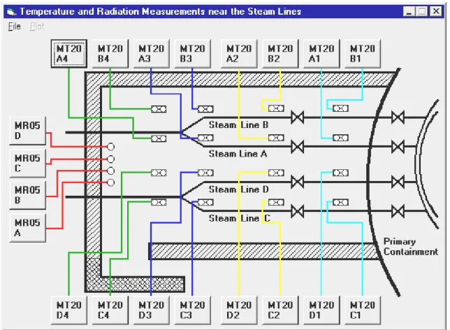
SensBase™ uses a GUI (Graphic User Interface) where transmitters with sensing lines and connections to the process are presented in graphic windows; see the window presented in Figure 4.1. This GUI is called “high pressure instrumentation for turbine”. The transmitters work like push buttons in the window in question. The graphic presentation of stored data is available for the user by pushing one or more transmitter buttons. There are in total 23 different GUI and these are used to cover the instrumentation at KKM. Every GUI covers a part of the instrumentation.
The turbine instrumentation in Figure 4.1 is valid for both turbine A and B at KKM. Letter A in the transmitter name refers to turbine A and letter B refers to turbine B. A transmitter with the name MP05B2 is a steam high-pressure transmitter for turbine B; see Figure 4.1. The GUI in SensBase™ shows that MP05B1 and MP05B2 are multiple with a common sensing line. The same holds true for the pair MP05B3 and MP05B4. It is also reasonable to expect that there is an agreement between the steam pressure pairs (MP05B1, MP05B3) and (MP05B2, MP05B4), since they record the steam pressure in the same stage of the process; see Figure 4.1.
4.1 Steam pressure transmitter MP05B2
In 1999, a deviating behavior was observed for the steam pressure transmitter MP05B2. Temporary changes in the signal mean value was observed. The deviations occurred intermittent. In Figure 4.2 an example from 2001 is shown. The signals MP05B2 and MP05B4 are recorded as a function of time in the figure and after 150 seconds there is a temporary reduction in pressure for MP05B2 that is not the case for MP05B4. MP05B2 and MP05B4 are connected to different pressure taps on the turbine according to the instrument system in Figure 4.1. Therefore it could not be excluded that the process caused the dip in pressure. Because of redundancy reasons it was unfortunately not
possible to record MP05B1 and MP05B2 during full power operation. Such a recording could have shown if the transmitter MP05B2 was deviating.
An investigation of the sensors was made based on measurement data collected during normal tests of the turbines A & B, when the reactor was no longer in power operation mode. A separate sensor recording was this time performed with the signals MP05A1 – MP05A4 and MP05B1 – MP05B4. During the measurement the steam pressure reference value was changed as the pattern shown in Figure 4.3 (turbine A) and Figure 4.4 (turbine B). Notice the good agreement between the steam pressure signals MP05A1 – MP05A4 for turbine A when the reference value is changed. The only deviation between the signals is a minor offset; see Figure 4.3.
The result for turbine B is shown in Figure 4.4. This figure displays that the pressure signals agree in the same way as for turbine A. Here, however, there is an interesting deviation. A sudden step shaped change occurs for MP05B2 after 120 s; see Figure 4.4. This shift is unique for the transmitter MP05B2. The interpretation is obvious. The transmitter MP05B2 has deviating dynamics.
The experiment has also been evaluated with the measures used in SensBase™. Gain, Offset and Amplitude ratio are used in SensBase™ for the comparison between time series. These measures can easily be explained with a graph where time series for the two signals are represented with the x- and y-axis. When two multiple signals are identical they form a straight line in the coordinate system with the slope = 1 and the extrapolation of the line passes origin. The relation between MP05B4 and MP05B3 are presented in Figure 4.5. The agreement between the signals is almost ideal. Gain is equal to the slope, deviation from origin the same as Offset and the deviation from the straight line is an Amplitude ratio measure.
These measures of comparison have been calculated for the signal pairs in Table 4.1 and 4.2. Gain is close to 1 for all comparisons while Offset is highest for the signal pair MP05B1 and MP05B2 in the tables. The Amplitude ratio valid for the different signal pairs is highest for MP05B1, MP05B2 where the figure 37.5 % is noted. The explanation for the high Amplitude ratio is evident from Figure 4.6, that presents MP05B2 as a function of MP05B1. The problem with MP05B2 causes the deviation from the straight line in the diagram.
Table 4.1 Gain, offset and amplitude ratio for the steam pressure signals in turbine B.
Parameters 031MP005B1/ 031MP005B2 031MP005B3/ 031MP005B4 Gain 0.9761 1.0010 Offset 1.5891 0.3709 Amplitude ratio 37.3 0.8176
Table 4.2 Gain, offset and amplitude ratio for the steam pressure signals in turbine A.
Parameters 031MP005A1/
031MP005A2 031MP005A3/ 031MP005A4
Gain 0.9809 1.0182
Offset 1.0758 -1.3822 Amplitude ratio 3.2830 0.3476
4.2 Exchange of the transmitter MP05B2
The transmitter MP05B2 was sent for service during the regular outage 2001. The report from service proves that there were interrupts in the electrical output from the transmitter. There was a crack on the electronic filter unit in the transmitter that could explain the sudden reductions in signal mean value; see figure 4.2. The exchanged filter unit is presented in Figure 4.7, observe the crack in the picture. Service documentation shows that it was necessary to replace certain mechanical and electronic parts of the transmitter.
Figure 4.1 The instrumentation for steam pressure measurements in turbine A and B at KKM.
0 50 100 150 200 250 300 350 68.4 68.45 68.5 68.55 68.6 68.65
68.7 Time series data for file; KKMJ_2.dat
Time [sec] P h ysical Unit 031MP0005B2 031MP0005B4 Figure 4.2 MP05B2 and MP05B4 as a function of time. KKM, 2001. 0 100 200 300 400 500 600 700 68 68.2 68.4 68.6 68.8 69 69.2 69.4 69.6 69.8 70
Time series data for file; KKMHH_1.dat
Time [sec] Ph ysi ca l U ni t 031MP005A1 031MP005A2 031MP005A3 031MP005A4 Figure 4.3 MP05A1-MP05A4 as a function of time during the experiment. KKM, 2001 0 100 200 300 400 500 600 700 68.2 68.4 68.6 68.8 69 69.2 69.4 69.6 69.8
Time series data for file; KKMHH_1.dat
Time [sec] Ph ysi ca l U ni t 031MP005B1 031MP005B2 031MP005B3 031MP005B4 Figure 4.4 MP05B1-MP05B4 as a function of time during the experiment. KKM, 2001 68.6 68.7 68.8 68.9 69 69.1 69.2 69.3 69.4 69.5 69.6 68.2 68.3 68.4 68.5 68.6 68.7 68.8 68.9 69 031MP005B3 031MP005B4 file KKMHH_1 Figure 4.5 MP05B4 as a function of MP05B3 during the experiment. KKM, 2001. 68.3 68.4 68.5 68.6 68.7 68.8 68.9 69 69.1 68.4 68.5 68.6 68.7 68.8 68.9 69 69.1 69.2 031MP005B1 031MP005B2 file KKMHH_1 Figure 4.6 MP05B2 as a function of MP05B1 during the experiment. KKM, 2001.
Figure 4.7 The electronic filter unit from the transmitter MP05B2.
5 Methods of investigating temperature sensors
Temperature signals normally include very little noise. There are many reasons for this. One explanation can be that the process is regulated in such a way that it only accepts very small fluctuations in temperature. Another reason can be that the measurement is filtered. An air temperature sensor that is constructed with a lot of metal will not react on small fast temperature fluctuations, for example. The real temperature is filtered by the construction of the sensor in such a way that only the mean value and the low frequency changes in temperature influence the measurement signal. The filtering also implies that a fast change in air temperature will be recorded by the measurement system with a time delay.
This chapter describes methods of investigating temperature sensors used at KKM. The first type of sensor measures air temperature while the other records water temperature in an emergency cooling system in the plant.
5.1 Investigation of air temperature
Steam lines at KKM are surrounded by temperature sensors in the so-called steam tunnel; see Figure 5.1. In this part of the reactor construction, where the external main steam line valves are installed, the aim with temperature measurement system is surveillance of leakage. They are in total 16 sensors of the RTD (Resistance Temperature Detector) type; see Figure 5.1.
These temperature sensors are tested in connection to the regular outage by being manually exposed to cooling spray. The cooling spray wets the temperature sensors and vaporizes. This process gives a fast reduction in temperature; see Figure 5.2. The reduction in temperature stops when the sensor is dry and all liquid has evaporated. Thereafter the temperature rises to the original temperature. The air temperature is the driving source of the increasing sensor temperature; therefore it is clearly slower than the cooling process. Figure 5.3 displays the temperature as a function of time during the cooling and natural heating of the sensor.
Used response times during cooling and reheating are defined in Figure 5.2 and 5.3. Cooling corresponds to the total temperature reduction that is 100 % and the cooling time is calculated to be between 10 % and 90 %; see Figure 5.2. Time for reheating is calculated to be from the point where the temperature starts to increase, just above 0 % in the Figure 5.3, until it reaches 63 % of the final value. The investigation is repeated every year and the results are stored.
5.2 Investigation of the temperature sensors in torus
Below the reactor at KKM there is a water filled torus shaped suppression pool, which is used in connection with emergency cooling. Steam can be transferred down into the torus to be condensed during an emergency. To supervise the torus, 12 temperature sensors, so-called RTD:s (Resistance Temperature Detectors), are mounted in thermo-wells in the torus; see Figure 5.4.
temperature sensor is carried out every year to investigate the dynamics. The individual temperature sensor is dismounted from its thermo-well and entered into a bucket with ice and water. When the temperature is stabilized at zero degrees the temperature sensor is dried and remounted into the thermo-well. This is performed during full power operation of the reactor. Sampling of the measurement signals is performed continuously during the experiment. The experiment is repeated for all 12 temperature sensors.
The temperature during the experiment is presented in Figure 5.5. The cooling is a fast process. According to the diagram, temperature reduces from 24 degrees down to almost zero in between 700 to 800 seconds. The time constant for the temperature reduction is calculated as the time it takes for the temperature to lose 63 % of the total temperature reduction. This is the most common definition of the time constant. The horizontal arrow during the temperature reduction in Figure 5.5 represents the 63 % level. This is from a physical point of view the time constant for the RTD-element with belonging electronics. The numerical values prove that the time constant for the temperature reduction is about 10 s.
A temperature increase with longer time constant (about 60 s) than during cooling is observed when the temperature sensor is reinstalled in the thermo-well; see Figure 5.5. The horizontal arrow during temperature increase defines the 63 % level. The water in the torus tank heats the RTD-element via the thermal resistance between the RTD and the thermo-well.This results in a clearly slower response time.
It is interesting that both time constants can be used for diagnosis. Deviations in the RTD-element and the sensor electronics are correlated with the cooling time constant. The time constant during heating indicates if there is rubbish or oxide between the RTD-element and the thermo-well. The experiment is also partly a calibration of the temperature sensor in the range 24 – 0 degrees.
Figure 5.6 displays results from the experiments with SensBase™. The two bar graphs in the bottom display the initial temperatures (Highest temperature) and the cooled temperature (Lowest temperature) in the torus tank for a temperature sensor from the years 1997-2000. It is evident from the bar graph that the torus temperature is between 21 and 25 degrees while the cooled temperature fluctuates between zero and 1.1 degree. The two top bar graphs in Figure 5.6 display the time constants during heating (Time constant + thermo-well) and the time constants during cooling (Time constant RTD). The results for the time constants for heating are very smooth during the years (between 50-55 s), while corresponding time constants for cooling varies between 9 and 15 s.
Figure 5.1 Temperature measurement system at the steam lines. Figure from SensBase™ at KKM.
Figure 5.2 Graphic presentation of the temperature during cooling with spray. KKM, 2001.
Figure 5.3 Graphic presentation of the time constant estimate during reheating. KKM, 2001.
Figure 5.4 The position of the temperature sensors in torus at KKM. The twelve sensors are installed in thermo-wells.
600 700 800 900 1000 1100 1200 0 5 10 15 20 25
Time series data for 116MT0205E File; KKMU1.dat
Un
it (
°C)
Time [sec]
Figure 5.5 Calculation of the time constants during cooling and reheating after installation of the sensor in the thermo-well.
Figure 5.6 Time constants during cooling and reheating and the temperature in the thermo-well in torus and ice-water. Results from the years 1997-2000 with temperature sensor MT205E. Data from SensBase™ at KKM.
6 Conclusions
Mainly depending on the fact that the Swedish BWRs were constructed in the seventies and eighties, the instrument systems were originally designed with analogue technique. This is valid for transmitters as well as density converters, isolation amplifiers and regulators. Right now there is an ongoing modernization of the instrument systems in many plants and components are replaced by newly developed ones. This implies in many cases that analogue components are replaced by digital ones.
The delay time is the critical dynamic deviation between an analogue and a digital transmitter. A delay time of up to 200 ms has been observed for a digital transmitter (Hartmann & Braun ASK800) in comparison with an analogue one (Fujii). A long delay time is of course undesirable when the transmitter is part of the reactor protection system. It is therefore important to pay attention to the delay in respons when an analogue transmitter is replaced by a digital one. The laboratory tests also included a comparison between an old analogue density converter (Hartmann & Braun TZA2) and a new digital one (Hartmann & Braun TZA4). These results prove that the analogue unit is clearly faster than the digital. The response time from differential pressure to level signal was 50 ms for TZA2 and 250 ms for TZA4. Corresponding times with pressure as input and level as output was 50 ms for TZA2 and 900 ms for TZA4.
The report also includes an investigation of pressure transmitters of the type TDE220. The transmitters exhibited deviating dynamics during ordinary sensor tests. The laboratory test confirms the observed deviation in comparison with transmitters of other types. The construction with Bourdon tube is judged to be the reason for the deviations. The report also presents results from trouble shooting with steam pressure transmitters at KKM. It was possible to identify the intermittent sensor error with the aid of controlled pressure changes. Service of the transmitter pointed out a crack on the electronic filter unit. This was judged to be the reason for the intermittent signal interrupts.
Finally two possibilities used at KKM to investigate the dynamics of temperature sensors are described. Both methods are based on artificial cooling of the sensor. One of them is applied during power operation of the plant and the other during outage.
7 References
1 Bergdahl B.G. Investigation of sensors and instrument components in boiling water reactors. Results from Oskarshamn 2, Barsebäck 2 in Sweden and Kernkraftwerk Mühleberg in Switzerland. May 1998, SKI Report 98:22.
2 Bengt-Göran Bergdahl, Joakim K.-H. Karlsson, Ritsuo Oguma and Herbert Schwaninger. Experiences from sensor tests and the evaluation of long-term sensor performance using SensBase™. Paper presented at the NPIC & HMIT 2000 meeting, Washington, DC, November, 2000.
3 B.G. Bergdahl, M. Morén and R. Oguma. Experiences from sensor tests and evaluation of sensor performance. Paper presented at SMORN VIII, Symposium On Nuclear Reactor Surveillance And Diagnostics, May 27 – 31, 2002, Göteborg, Sweden.
4 IAEA-rapport. Management of ageing of I & C equipment in nuclear power plants. Report prepared within the framework of the International Working Group on Nuclear Power Plant Control and Instrumentation. June 2000. IAEA-TECDOC-1147.
5 Bergdahl BG, Liao B, Oguma R, Schwaninger H. Sensor diagnostics in a BWR based on noise analysis. An invited paper presented at the NPIC & HMIT’96 meeting May 6 - 9, 1996, The Pennsylvania State University, USA.
6 Hashemian HM et al. Effect of Aging on Response Time of Nuclear Plant Pressure Sensors. Analysis and Measurement Services Corporation. NUREG/CR-5383.
7 Hashemian HM et al. Long Term Performance and Ageing Characteristics of Nuclear Plant Pressure Transmitters. Analysis and Measurement Services Corporation. NUREG/CR-5851.
SKI Report 2005:36
Research
Reports within the Area of Nuclear Power
Plant Instrumentation
Part 2: Dynamic Deviations in Reactor Pressure and
Water Level Signals Caused by Sensing Lines
Bengt-Göran Bergdahl
GSE Power Systems AB
Box 62
611 22 Nyköping
November 2004
SKI Project Number XXXXX
This report concerns a study which has been conducted for the Swedish Nuclear Power Inspectorate (SKI). The conclusions and viewpoints presented in the report are those of the author/authors and do not necessarily coincide with those of the SKI.
Abstract
Sensors are a part of the safety system in a reactor. They are the first link in a chain of components that influence the protection system. It is therefore of great importance that the sensors fulfill the requirements on reliability and response time. The dynamic character of sensors is in practice seldom or never tested in BWRs. The static performance is on the other hand tested every year during the calibration of the transmitters. This is performed during the regular outage of the reactor.
It is quite common that many transmitters are connected to the same sensing line. This is especially valid in old reactors where only a few number of pressure taps are available on the reactor vessel. This is a shortcoming in the construction since one fault in the sensing line influences all connected components; a so-called CCF (Common Cause Failure).
The present report was sponsored by SKI (Swedish Nuclear Reactor Inspectorate). The report focuses on possible deviations in the sensing lines. The deviations are presented with practical examples from Swedish and foreign BWRs.
The sensing line and its belonging mechanical passive components can reduce the response time for a measurement system without influencing the static presentation. The report describes cases in a power plant where the response time was extended from 0.1 s to 5 s. The reason was gradual blockage in the sensing line. There is only one technique available today with which it is possible to investigate sensor dynamics, and that is signal analysis. Appropriate analysis of the transmitter signals can reveal filtering whether it takes place in the sensing line, the transmitter or in the electronic instruments.
As an example a practical case is presented where pulsation dampers with so-called needles were used at Ringhals 1 in Sweden. Their influence on the response time for the measurement signal corresponded to a time constant of 0.55 seconds. By eliminating the needles the requirements on the response time was fulfilled.
Results from KKM (Kernkraftwerk Mühleberg in Switzerland) show a way to supervise blockage in sensing lines based on the transmitter signal. One example is presented with a transmitter for flow measurement equipped with pulsation dampers. Results from SensBase™, a database system for sensor tests, is used in this work. SensBase™ stores new sensor test results every year. The nuclear power inspectorate in Switzerland has approved that KKM reduced their comprehensive transmitter calibration after introduction of the annular use of sensor tests and SensBase™.
The report also describes pressure oscillations that take place in the sensing line and not in the real measured process. The water in the sensing line together with the transmitter membrane form a dynamic system with water as mass, elasticity in the transmitter membrane as spring constant and reactor pressure fluctuations as driving force. The problem with oscillations in the measurement system is illustrated with examples from Ringhals 1 and KKM.
One example is also presented from KKM where the oscillation in a level transmitter – a Barton Cell – influenced eight transmitters connected to a common sensing line. It was possible to identify the deviating transmitter during operation of the reactor via
experiment with isolation valve closing. The oscillations ceased after replacing the transmitter with one with less volume and displacement.
The report finally proves that mechanical vibrations in the sensing lines contribute to signal noise around 10 Hz. This is shown with the aid of laboratory tests performed at KKM. Transmitters have also been exchanged because of deviating noise in the frequency range 2-20 Hz. After replacing the transmitter the mentioned noise disappeared. The results from KKM indicate that it cannot be excluded that ageing increase the transmitter sensitivity for sensing line vibrations.
Table of contents
1 Background 7
2 Water level changes in the condensate pot 8
3 Gradual blockage, gas or freezing in a sensing line 11
3.1 The sensing line and its components 11
3.2 Air or gas in sensing line 12
3.3 Freezing or gradual blockage in the sensing line 12 3.4 Pulsation damper compared with electronic filtering 13
3.5 Conclusions for the dynamics in sensing line 13
4 Oscillations in reactor pressure signals at Ringhals 1 16 5 Differential pressure sensors with and without needles in the pulsation dampers
in Ringhals 1 20
6 Pulsation dampers in sensing lines in jet pump flow measurement system at
KKM 24 7 Oscillation in a water level transmitter with influence on others 27
7.1 The decision to close valves on the sensing lines to ML93 and ML94A 27
7.2 Exchange of transmitter ML93 29
8 Reactor pressure and reactor water level with 10 Hz noise 34 8.1 Experiments with sensing line vibrations at KKM 34 8.2 MP34B2 before and after the exchange of transmitter observed with
SensBase™ 35
9 Conclusions 39
1
Background
Sensors are part of the protection system in a reactor. They are the first link in the chain that influences the protection system. It is therefore of importance that the sensors fulfill the demands of reliability and response time. In practice, the dynamic characteristics of sensor systems are seldom or never tested in Swedish and foreign BWRs. The static character however, is tested by sensor calibration during the regular outage of the plant. Transmitters and other instrument components will be replaced by different models of components in an ageing nuclear power plant. This implies that different sensor types and models are in operation. Furthermore it is not unusual that complete systems with sensing lines are exchanged or rebuilt and newly-developed condensate pots are installed. This implies that the dynamic character during the test operation of the plant has changed.
The measurement systems for reactor pressure and water level in a BWR consists of transmitters connected to the pressure taps on the reactor vessel through water filled sensing lines. The transmitters are installed outside the containment where temperature and radiation is lower. Figure 2.1 shows such an installation at Barsebäck in Sweden. It is obvious from the figure that the sensing line from the pressure tap to the transmitter can be many tens of meters.
It is quite common that many sensors are connected to the same sensing line. This is especially the case in old reactors where only a few number of pressure taps are available on the reactor vessel. This is an inconvenient drawback in the construction since an error in the sensing line influences all connected components; a typical CCF. The high positioned taps on the reactor have condensate pots installed. This is to separate steam in the reactor from water in the sensing line. It is evident from the Figure 2.1 that the high positioned pressure taps in Barsebäck have up to 3 condensate pots connected to one pressure tap. This construction was made to improve the redundancy and reduce the described CCF.
The report is focused on deviations in the measurement system in connection to the sensing lines. The deviations are demonstrated with practical examples from Swedish and foreign power plants. The report was sponsored by SKI, the Swedish Nuclear Power Inspectorate.
The deviations treated in the report are:
• Changes in the condensate pot water level caused by gas in the reference sensing line.
• Increasing degree of blockage, influence by gas or freezing in the sensing line. • Not wanted oscillations that can take place in pressure and level measurements
caused by the mass of water in the sensing line and the spring constant in the transmitter.
• How can one oscillating transmitter have influence on the others connected to the same sensing line and at the same time filter fast pressure changes on multiple transmitters?
• The influence from pulsation dampers (snubbers) and other mechanical components in the sensing line on the signal response time.
The author of the report wants to express his thanks to Mr. Hashemian at AMS in the USA for stimulating discussions and exchange of experiences within the sensor test area. References with high importance on Chapter 2 and 3 in the report are Reference 6 and 7 (NUREG/CR-5383 and NUREG/5851).
Thanks also to Mr. Marcus Andersson who gave us the permission to publish the results from the GSE investigation at Ringhals 1. Thanks also to Mr. Herbert Schwaninger who gave us the permission to publish the results from KKM and also inspired the research with fruitful discussions. Thanks also to Jan-Ove Andersson for the permission to publish material from Barsebäck 2 and his contribution with valuable comments on the report.
2
Water level changes in the condensate pot
A principal picture for the transmitter and other components that can be connected to a sensing line for measurement of reactor pressure is presented in the Figure 2.3. Close to the pressure tap on the reactor vessel a condensate pot is connected. In this unit the water in the sensing line is separated from the steam in the reactor that exist on the level where the pressure tap is placed. Steam communicates via the pressure tap between the reactor and the condensate pot – where condensation is performed. Overflow of water in the pot will run back to the reactor. This is the way the water level in the pot is controlled.
Gas bubbles can arise in the sensing line, for example during pressure transients. They are transported to the condensate pot since the sensing line normally is constructed without horizontal slopes. An increasing gas content in the sensing line water increases the volume, so called swelling. As a result there will be overflow of water to the reactor from the condensate pot. When the formation of gas has ceased and the gas has been transported away there will be a clearly reduced water level in the condensate pot. This is especially a problem for the water level measurement in the reactor. These transmitters use dp measurement with the level in the condensate pot as a reference. The level measurement will deviate in the same way as the reference level changes. This type of error is well known. Some reactors have the possibility to refill the water level in the condensate pot during operation after such an event. This is done manually in this case.
Gas is transported together with steam to the condensate pot during normal operation. This gas is diluted in the sensing line water and as far as the gas is diluted there is no negative influence on the level measurement. But a pressure transient is enough to release the diluted gas to bubbles in the sensing line water.
Another thing is that non-condensable gas for example oxyhydrogen can be collected in the condensate pot. Such a gas can explode and influence all components connected to
developed to avoid collection of non-condensable gas. One type is more flat and without the sphere shape seen in Figure 2.3. The result is that the complete volume will be ventilated by steam. Such a construction has been chosen at KKM. There are also other solutions, for example the one used at Barsebäck 2. There the top of the condensate pot has been connected to the steam line with a pipe; see Figure 2.2. This is one way to evacuate steam as well as non-condensable gas and gas that can be diluted in the sensing line water. The result is reduced amount of diluted gas (or no gas at all) in the sensing line water. This is a way to reduce the risk for swelling during a reactor pressure transient.
Figure 2.1 Pressure taps, condensate pots and sensing lines for pressure and level measurement system in Barsebäck 2 in Sweden.
Condensate Pots Condensate
Figure 2.2 Condensate pots, sensing lines, pressure tap to the reactor vessel and exhaust gas pipe to the steam line at Barsebäck 2.
Condensate pot Sensing line Reactor vessel Containment wall Restriction device Isolation valve Pulsation damper Displacement volume Transmitter Electro mechanical part Electronic filter
Figure 2.3 Reactor pressure instruments. The figure displays sensing line, pressure tap, condensate pot, restriction device, containment wall, manual isolation valve, pulsation damper (snubber) and transmitter.
Condensate pot Sensing line Connection to the reactor vessel Exhaust gas pipe
3
Gradual blockage, gas or freezing in a sensing line
The aim with the sensing line is to transfer the pressure at the pressure tap to the transmitter membrane without inconvenient filtering; see Figure 2.2. This is not always successful. The components that are part of the measurement system can filter the pressure fluctuations by gradual blockage of the water in the sensing line. Some times the gradual blockage can also increase caused by crud – a chemical process in the sensing line water.
Gradual freezing of the sensing line water has a filtering influence similar to the description of gradual blockage.
Gas bubble in sensing lines also have dynamic influence on the pressure signal that will be transferred to the transmitter membrane. The pressure transmitter signal will be presented with time delay during a real pressure transient as a result of the filtering. This chapter will present these types of problems and suggest actions to be taken to reduce their influence on the response time.
3.1 The sensing line and its components
The sensing line and its components for pressure measurements are displayed in Figure 2.2. Besides pressure tap and condensate pot that already has been discussed in the report there are also further components. To them belong the units called restriction device, isolation valve, pulsation damper and transmitter.
The restriction device is a mechanical unit with the task to stop the leakage of reactor water if a sensing line ruptures. The restriction device will not filter the transmitter signal during normal operation. International reports recommend that restriction devices should be avoided in measurement systems that demands short response times; see Reference 7. The same thing holds true for the isolation valve installed on the sensing line. This unit is also not meant to influence the measurement signal. The valve in question is meant to be used for closing of the sensing line e.g. during exchange of transmitter.
Pulsation dampers may also be installed in the sensing line. Such a unit is displayed in Figure 2.2. The pulsation damper works like a mechanical restriction in the sensing line. The constructions can differ. One design is an axial pipe installed in the sensing line where so-called needles can be inserted. It is possible to achieve different restrictions by choosing the size of the needle. The task for this unit is mechanical filtering of the pressure to the transmitter. This was a common way to filter signals in the seventies and eighties but the method has obvious drawbacks. These will be described later in the report. NRC (Nuclear Regulatory Commission) in USA recommends the utilities not to use pulsation dampers for filtering.
The transmitter is installed in the end of the sensing line. This unit consists of a water filled volume that influences the transmitter membrane. The response from the membrane is a movement that increases the volume. This increase in volume is called transmitter displacement. An increased pressure results in increasing volume achieved by movement of the membrane; see Figure 2.2. The movement of the membrane in its turn influences the electro mechanical system, which transfer the membrane position to