DEGREE PROJECT, IN COMPUTER SCIENCE , FIRST LEVEL STOCKHOLM, SWEDEN 2015
A comparative study of hybrid
artificial neural network models for
one-day stock price prediction
JOY ALAM AND JESPER LJUNGEHED
A comparative study of hybrid artificial neural
network models for one-day stock price prediction
JOY ALAM AND JESPER LJUNGEHED
Degree Project in Computer Science, DD143X
Supervisor: Alexander Kozlov
Abstract
Prediction of stock prices is an important financial problem that is receiving increased attention in the field of artificial intelligence. Many different neural network and hybrid models for obtaining accurate predic-tion results have been proposed during the last few years in an attempt to outperform the traditional linear and nonlinear approaches.
This study evaluates the performance of three different hybrid neu-ral network models used for one-day stock close price prediction; a pre-processed evolutionary Levenberg-Marquardt neural network, Bayesian regularized artificial neural network and neural network with technical-and fractal analysis. It was also determined which of the three outper-formed the others.
The performance evaluation and comparison of the models are done using statistical error measures for accuracy; mean square error, symmet-ric mean absolute percentage error and point of change in direction.
The results indicate good performance values for the Bayesian regu-larized artificial neural network, and varied performance for the others. Using the Friedman test, one model clearly is different in its performance relative to the others, probably the above mentioned model.
The results for two of the models showed a large standard deviation of the error measurments which indicates that the results are not entirely reliable.
Sammanfattning
Prognoser av aktiepriser ¨ar en viktig finansiell uppgift som f˚ar allt mer ¨
okad uppm¨arksamhet inom artificiell intelligens. M˚anga artifiella neu-ronn¨at och hybrida modeller med syftet att erh˚alla noggranna prognoser har introducerats de senaste ˚aren i ett f¨ors¨ok att ¨overtr¨affa de traditionella linj¨ara och icke-linj¨ara metoderna.
Denna studie unders¨oker precisionen hos tre olika hybrida artificiella neuronn¨atsmodeller modeller som anv¨ants inom endags-aktieprisprognoser; ett evolution¨art f¨orbehandlat artificiellt neuronn¨at, ett bayesianskt normerat artificiellt neuronn¨at och ett artificiellt neuronn¨at i kombination med teknisk- och fraktal analys. Vilken av dessa som presterar b¨attre ¨an de andra har ¨aven unders¨okts.
De olika modellerna evalueras och j¨amf¨ors med hj¨alp av tre statistiska metoder f¨or att best¨amma noggrannheten: medelfelen i kvadrat, sym-metriska medelfelet relativt absolutfelet och en metod f¨or att m¨ata hur tv˚a kurvor f¨orh˚aller sig till varandra med avseende p˚a riktning.
Resultaten indikerar god precision f¨or det bayesianskt normerade neu-ronn¨atet, och varierad noggrannhet f¨or de andra. Anv¨andning av Fried-man testet visar att en av modellerna klart ¨ar annorlunda ¨an de andra, troligen det bayesianskt normerade neuronn¨atet.
Resultaten f¨or tv˚a av modellerna visade en stor standardavvikelse p˚a v¨ardena fr˚an de statistiska metoder anv¨anda f¨or att best¨amma nog-grannheten vilket inneb¨ar att resultaten inte ¨ar p˚alitliga.
CONTENTS
Contents
List of Figures 5 List of Tables 5 Acronyms 6 1 Introduction 7 1.1 Problem statement . . . 8 1.2 Scope of study . . . 81.3 Disposition of the report . . . 8
2 Background 9 2.1 The stock market and prediction methods . . . 9
2.2 Artificial intelligence . . . 10
2.2.1 Artificial intelligence in stock market prediction . . . 10
2.3 Artificial neural networks . . . 10
3 The models being compared 13 3.1 Bayesian regularized ANN . . . 13
3.2 Combining fractal analysis with technical analysis and ANN . . . 14
3.3 A pre-processed evolutionary Levenberg-Marquardt neural net-work model . . . 15
3.4 Indicators used in technical analysis prediction . . . 17
3.4.1 Bias . . . 17
3.4.2 Exponential Moving Average . . . 17
3.4.3 Relative strength index . . . 17
3.4.4 Rate of change . . . 17
3.4.5 Stochastic oscillator . . . 17
3.4.6 Bollinger oscillator . . . 17
3.4.7 Advance/Decline Line . . . 17
3.4.8 Moving Average Convergence Divergence . . . 18
3.4.9 Williams %R . . . 18
4 Method 19 4.1 Data selection . . . 19
4.2 Performance measures . . . 20
4.2.1 Mean Squared Error . . . 21
4.2.2 Symmetric Mean Absolute Percentage Error . . . 21
4.2.3 Point Of Change In Direction . . . 21
4.3 Detecting differences - the Friedman test . . . 22
5 Results 23 5.1 Models benchmarked on Microsoft stock price data . . . 23
5.2 Models benchmarked on S&P500 data . . . 25
CONTENTS
6 Discussion 29
6.1 Discussion of results . . . 29 6.2 Discussion of method . . . 30 6.3 Discussion of reviewed studies . . . 31
7 Conclusion 31
7.1 Future research . . . 31
8 Bibliography 33
Appendices 37
Appendix A A more thorough background of genetic algorithm 37 Appendix B Detailed results of models benchmarked on MSFT 37 Appendix C Detailed results of models benchmarked on SNP 39
LIST OF TABLES
List of Figures
2.1 Model of a neuron in the human brain with its most important parts. Source www.forskerfabrikken.no/fasinerende-hjerneceller/ 11 2.2 4-5-1 architecture MLP neural network model (4 input nodes, 5
hidden nodes and 1 output node). Source: dmm613.wordpress.com/2014/12/16/demystifying-artificial-neural-networks-part-2 . . . 11
4.1 The datasets used for training, validation and testing. . . 20 5.1 Actual and predicted closing stock prices using BRANN on MSFT
for the test period. . . 23 5.2 Actual and predicted closing stock prices using FTANN on MSFT
for the test period. . . 24 5.3 Actual and predicted closing stock prices using PELMNN on
MSFT for the test period. . . 24 5.4 Actual and predicted closing stock prices using BRANN on SNP
for the test period. . . 26 5.5 Actual and predicted closing stock prices using FTANN on SNP
for the test period. . . 26 5.6 Actual and predicted closing stock prices using PELMNN on SNP
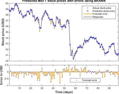
for the test period. . . 27 B.1 Actual and predicted closing stock prices with prediction errors
using BRANN on MSFT for the test period. . . 37 B.2 Actual and predicted closing stock prices with prediction errors
using FTANN on MSFT for the test period. . . 38 B.3 Actual and predicted closing stock prices with prediction errors
using PELMNN on MSFT for the test period. . . 38 C.1 Actual and predicted closing stock prices with prediction errors
using BRANN on SNP for the test period. . . 39 C.2 Actual and predicted closing stock prices with prediction errors
using FTANN on SNP for the test period. . . 39 C.3 Actual and predicted closing stock prices with prediction errors
using PELMNN on SNP for the test period. . . 40
List of Tables
3.1 Features of GA used in ENN . . . 16 4.1 Input stock data . . . 20 5.1 Performance measures using different models on MSFT stock data 25 5.2 Standard deviations of performance measures on MSFT stock data. 25 5.3 Errors using different models on SNP stock data . . . 27 5.4 Standard deviations of performance measures on SNP stock data. 28
Acronyms
Acronyms
AD Advance/Decline Line. 13, 16 AI Artificial Intelligence. 9 ANN Artificial Neural Network. 6 BIAS N-day Bias. 16
BO Bollinger Oscillator. 13, 16 BP Backpropagation. 11
BRANN Bayesian Regularized ANN. 12 EMA Exponential Moving Average. 13 ENN Evolutionary Neural Network. 14 FFNN Feed-Forward Neural Network. 10 FRAMA Fractal Analyis Moving Average. 13
FTANN Fractal analysis and Technical analysis ANN. 13, 18 GA Genetic Algorithm. 6
LM Levenberg-Marquardt. 11
LMBP Levenberg-Marquardt Backpropagation. 11 MACD Moving Average Convergence Divergence. 13, 17 ML Machine learning. 9
MLP Multilayer Perceptron. 10 MSE Mean Squared Error. 7
MSFT Microsoft Corporation stock price. 18
PELMNN Pre-processed Evolutionary Levenberg-Marquardt ANN. 14, 18 POCID Point Of Change In Direction. 7
RMSE Root Mean Square Error. 14 ROC Rate Of Change. 13, 16 RSI Relative Strength Index. 13
SMAPE Symmetric Mean Average Percentage Error. 7 SNP S&P500 index. 18
1 INTRODUCTION
1
Introduction
Prediction of stock prices is an important activity performed by investments banks and private investors. To maximize profit and minimize risk from stock trading; prediction is a vital part [1]. Several methods are used to aid in the pro-cess of prediction including fundamental analysis, technical analysis and techno-logical prediction. Prediction is a complex and difficult task because of several dynamic factors, both economic and non-economic, in combination with the volatility of the market prices [2].
Technological prediction is the use of artificial intelligence to predict stock prices. The key for better prediction is to further improve the prediction of finan-cial time series. As of late, a lot of research has put efforts into proper characteri-zation, modeling and prediction of financial time series. Popular methodologies applied to stock market prediction are fuzzy systems [3], Genetic Algorithm (GA), regression analysis and support vector machines [4]. Hybrid models, i.e. models that combine methodologies, are also a common approach to prediction that has shown mixed results [5][6][7][8][9].
Artificial Neural Network (ANN) is another popular model in stock mar-ket prediction from the field of machine learning [1][10][11][12]. An ANN has several desirable characteristics (nonlinear, self-adaptive and non-parametric) making it appropriate for prediction with complex underlying properties [9]. However, making decisions based solely on ANN prediction has been argued to be insufficient [13], why hybrid models are under study.
Hybrid models are approaches combining two or more components in order to make use of the advantages of each component and to cover the shortcomings of one another. In literature, there exists many hybrid based models where one component is an ANN. Asadi et al. (2012) proposed an pre-processed evolution-ary Levenberg-Marquardt ANN model. Paluch and Jackowska-Strumillo (2014) proposed a hybrid ANN model using fractal analysis. Ticknor (2013) proposed a model combining Bayesian regularization, ANN and common technical indi-cators, which may not be seen as a hybrid ANN model but will be addressed as one throughout the study.
In most cases the conclusion of studies in this field are that the proposed hybrid models are superior to the components used by themselves. Guresen et al. (2011) conducted a comparative study which included several hybrid mod-els. The conclusion of the study was that a dynamic ANN [15] proposed 2005 had the best predictive performance. Since then, there are few studies compar-ing the most recent hybrid ANN models to each other, where this comparative study is filling a gap. The of aim of this study is to try some recent hybrid ANN models to estimate the progress of one-day stock price prediction models.
1 INTRODUCTION
1.1
Problem statement
This report investigates some recent proposed hybrid ANN models. As the ar-ticles proposing these models often compare with outdated models, the goal of this study is to compare recent ones by answering the following question:
How does the recent hybrid ANN models; pre-processed evolutionary Levenberg-Marquardt ANN, Bayesian regularized ANN and technical and fractal analysis ANN; perform in accuracy on one-day stock price prediction on the same input data and which of these gives the most promising results?
1.2
Scope of study
The analysed models will be tested on S&P500 index and Microsoft stock prices. The performance of the models will be compared using Mean Squared Error (MSE), Symmetric Mean Average Percentage Error (SMAPE) and Point Of Change In Direction (POCID).
This study is restricted by a number of factors, such as resources. These will limit the study to be completely comparative and there will be no thorough analysis to why one model performs better than another. The choice of mod-els and parameters for the network architectures will be made based on other studies, thus requiring extensive literature studies. The prediction will be one day in the future, called one-day prediction throughout this study.
Statistical methods such as standard deviation will be used for trying to determine the reliability of the results and the Friedman test will be used to determine if a model is different than the others. A multiple comparison test, to determine which model is different, is not conducted.
Because of the restrictions in knowledge of the area of AI and ANNs and the time constraint, the models will be implemented with the use of a high level language. This will enable easy data processing, modifications of the models and plotting results.
A great limitation on the study is a few iterations performed by each model due to one of the models taking a considerate amount of time to run.
There will be no guidelines on how well these models would actually aid in earning money when used on a actual stock market.
1.3
Disposition of the report
The remainder of this report is organized as follows: section two will present some background required to understand the study of ANNs in stock market prediction and also present topics regarding the hybrid models. The third sec-tion will present the studies from where the models which are to be compared have been chosen. The fourth section describes the choice of data and how the performance will be measured. The fifth section presents the predictions made by the models and compare their performances. The sixth section presents why the results have been obtained, what might have affected the results and how the methods where conducted. The last section summarizes and concludes this study.
2 BACKGROUND
2
Background
This section will briefly present the stock market, different prediction methods and more specifically methods from the field of artificial intelligence.
2.1
The stock market and prediction methods
When a company need to raise money to expand they can borrow from an external part or raise it from investors by selling them a stake in the company. That stake in the company is sold by issuing stock in the form of shares which makes the buyer a part owner in the company with a claim on assets and profits. A stock is concisely a share of ownership [16].
A stock market is an organized market for the sale and purchase of shares and stocks. The functions of a stock market varies between countries but there are two general important functions. Ensuring the liquidity for stocks and en-couraging people to invest saving into corporates, and allocating capital among firms by determining prices reflecting the actual investment value of a com-pany’s stock. A market is made by matching customer orders with the best price available [17].
The price of a stock is constantly updated with each trade taking place. The market price at which the buyer and seller agrees to trade is the price of a stock at the moment. While the market is being open during a day the price will fluctuate depending on the trading prices. The price that a buyer and seller are willing to bid and ask for are dependent on market forces, supply and demand of stocks. The supply of stock are the number of shares a company has issued. Those who wants to buy shares from owning investors creates the demand [18]. The open price is the price of the first trade of a trading day, close price is the price of the last trade. Low- and high price are the lowest and the highest of prices of a trade during a day.
What is considered to be a reasonable price to sell and buy a stock are influenced by several factors. The New York Stock Exchange [18] presents four such factors that influence buyers and sellers.
• The health of a companys’ finances influence demand and supply. The past performances and its future prospects indicates how well the company is doing.
• Information about the industry the company is active in might influence its stock price.
• Economic trends are general trends that signal changes in the economy of a country.
• World or national events can affect stock prices when investors believe a new event may be good or bad for the economy.
Apart from these, there are many factors influencing the stock market. There are three broad categories in which stock prediction can be categorized; funda-mental analysis, technical analysis and the use of technological methods. Funda-mental analysis analyzes the company underlying the stock, and tries to predict using past and present data about the company. The market, health of the
2 BACKGROUND
company, competitors and financial statements are analyzed. In technical anal-ysis, technical indicators are data derived from the technical data such as open, close and low prices. Technical indicators are used to analyze the stock market with respect to trend and overbought or oversold situations. Technical indica-tors uses past data in order to predict future behaviour of the stock market. Technological methods relies mainly on artificial intelligence for trying to learn the underlying complex factors when predicting stock prices.
2.2
Artificial intelligence
Artificial Intelligence (AI) is the study of intelligent machines, with the main focus on intelligent computer programs. Some activities that computers with ar-tificial intelligence are designed for are learning, reasoning, planning, perception and natural language processing [19].
Machine learning (ML) is one core branch of AI. It is the study of algorithms that improves itself through experience. The learning is done by applying statis-tics and mathematical optimization on input data [20]. ML tasks can be divided into three learning paradigms depending on the feedback available to a learning system, supervised learning, unsupervised learning and reinforcement learning [19].
Supervised learning algorithms are presented with some example inputs (training data) and the desired output. The learning algorithm learns a gener-alized rule from the training data which maps to the outputs. The goal is for the algorithm to create such a rule that it will be able to predict future values depending on new input data. Such prediction methods can be used in a wide range of areas, such as weather forecasting, housing prices, and stock prediction. ANNs are included in the task of supervised learning.
2.2.1 Artificial intelligence in stock market prediction
A prediction algorithm uses a set of known entities to produce a prediction of future values for the same or other entities. When it comes to stock market prediction, the entities can be divided into two categories, namely pure technical data and fundamental data [21]. Technical data is a stocks closing, high and low prices and volume. Fundamental data are the factors described in section 2.1. The goal for an AI prediction algorithm is often to predict future close price for stocks.
2.3
Artificial neural networks
ANNs are biologically inspired statistical learning algorithms applied to predic-tion of time series [9], mimicking the neural network in our brains which consists of billions of neurons [22]. A neuron has a cell body, dendrites, an axon and synaptic terminals, fig. 2.1. The cell body, receiving synapses (electrical im-pulses) through dendrites is activated and emits a signal through the axon when the synapses surpass a certain threshold. The receiving synapses have variable strengths meaning that some signals contribute more to the activation of the neuron. The emitted signal might be sent to other neurons activating them and creating a chain of synapses [23].
2 BACKGROUND
Figure 2.1: Model of a neuron in the human brain with its most important parts. Source www.forskerfabrikken.no/fasinerende-hjerneceller/
A variety of problems in pattern recognition, predition, optimization, as-sociative memory and control are solved by ANNs [24]. ANNs are highly ab-stracted and modeled in layers in contrast to the complex biological neural network. ANNs consists of an inter-connection of some number of neurons.
ANNs can be seen as weighted directed graphs. The connection pattern (architecture) of the ANN can be grouped into two categories; Feed-Forward Neural Network (FFNN) (graphs with no loops) and recurrent (or feedback) neural networks (graphs with loops). Multilayer Perceptron (MLP), a FFNN, is the most common architecture [24]. A MLP consists of one input layer, one or more hidden layers and one output layer. The first layer (the input layer) consists of one or more inputs. An input is a vector of values. Every node in the input layer is connected to the nodes of the first hidden layer. The data flows forward in the network through the hidden layers until the output layer is reached as can be seen in fig. 2.2.
Figure 2.2: 4-5-1 architecture MLP neural network model (4 input nodes, 5 hidden nodes and 1 output node). Source: dmm613.wordpress.com/2014/12/16/demystifying-artificial-neural-networks-part-2
Each artificial neuron in the network is represented by some directed edges (connections between neurons in different layers), a node and a
mathemati-2 BACKGROUND
cal function. The inputs (like synapses) to a node are multiplied by adaptive weights (like the strength of the respective signals) and activates the neuron if the sum of the inputs satisfy a mathematical function [23]. Different mathemat-ical functions are used to indicate whether a neuron is activated. Some of these functions include the threshold, piecewise linear and, most frequently used, the sigmoid function [24]:
Sigmoid function ϕ(t) = 1
1 + e−t (2.1)
The ability to learn for an ANN is by updating the network architecture and connection weights. The network must learn and adjust the weights iteratively from available training techniques, which improves the performance. The ANN learns a rule, like a input-output relationship, from example data [24].
The nodes with their respective function process the information received by the input nodes. The applied weights to each connection represents the signif-icance in terms of impact on output nodes the information stored in the node has. These nodes are then trained to determine significant nodes. The most popular training technique is Backpropagation (BP). The BP process works as follows: the output values are compared with the actual values to compute the value of some predefined error-function. This error function is typically the MSE (defined by equation 4.1).
By various techniques, Levenberg-Maurquardt [25] being the one used by most ANNs in this study, the error is fed back through the network. The Levenberg-Marquardt (LM) (LM and Levenberg-Marquardt Backpropagation (LMBP) will be interchangably used in this study) algorithm is a hybrid op-timization technique which combine the positive attributes of Gauss-Newton algorithm and gradient descent algorithms. Using the error information, the algorithm adjusts the weights of each connection in order to reduce the value of the error function by some small amount. After repeating this process for a sufficiently large number of training cycles (epochs), the network will usually converge to some state where the error of the calculations is small.
For an ANN to learn, it is presented with an amount of data called the training data. The training data is used to adjust the weights on the neural network. On each epoch, the ANN has some amount of validation data on which it predicts and calculates an accuracy measure to assess the performance on data which it has not trained on. This is done to avoid overfitting (avoid that an increase in accuracy over training data gives a decrease in accuracy over validation data). The testing set is where the ANN will predict in order to confirm the actual predictive performance of the ANN model.
The popularity of MLP can be explained by the network’s ability to learn complex relationships between input and output patterns, which could be diffi-cult to model with conventional algorithmic methods [5][24].
3 THE MODELS BEING COMPARED
3
The models being compared
To predict stock prices, one of the best ways is by using ANNs which are good at adapting to the changes of the market. In later years, several techniques have been combined with neural networks to improve its predictive capabilities. Some of these are fuzzy logic, genetic algorithms, biologically based algorithms among others [7].
Among all different combinations of hybrid models the three models used for comparison in this study are introduced shortly in this section. For fur-ther details and mathematical explanations it is recommended to investigate the articles further. The implementations of the models in this study are those parameters introduced below, with any deviation being noted. Technical indi-cators used by the models are shortly introduced at the end of this section.
3.1
Bayesian regularized ANN
Bayesian Regularized ANN (BRANN) proposed by Ticknor (2013) is a three layered feedforward ANN using Bayesian regularization in the BP process, used for one-day stock price prediction. It is a hybrid in the sense that it uses ANN in combination with technical analysis. This model is of interest in this study because of the use of a non-traditional training algorithm for stock prediction.
This hybrid was proposed in order to reduce the potential of overfitting and overtraining when using conventional learning techniques, as the Levenberg-Marquardt training algorithm. Bayesian regularization developed. It is a math-ematical technique which converts nonlinear systems into ”well posed” problems. Bayesian regularization adds an extra term to the error function that is to be reduced during training. In complex models, which is often the case with stock market prediction, unnecessary weights between neurons are driven to zero and the network will train on the nontrivial weights. The goal is to increase the generalisation of the network by not finding a local minima as the optimal for the weights, instead looking for the global minima.
There were two experiments conducted by Ticknor. The first one to deter-mine the number of neurons to be used in the hidden layer and testing it on two input data sets, Microsoft and Goldman Sachs. In the other experiment the proposed model was compared to a complex hybrid model.
Empirically adjusting the number of hidden neurons between 2 and 10 until the effective number of parameters reached a constant value, it was determined that the hidden neurons should be 5. The BRANN provided on average a ¿98% for both stocks over the total trading period. It managed to handle noise and volatility without overfitting the data.
In the comparison study, the number of hidden neurons used was determined to be 20 after a thorough analysis. The models were both run on two input sets of 492 trading days each (Apple and IBM), and of which approximately 18% were for testing. The input sets where those used in the study of the more complex model. Performance was measured using the mean absolute percentage error. The results indicate that the BRANN is as good as the complex model, recieving better results on one of the sets. It provides a simplified prediction tool compared to similar complex neural network techniques.
Inputs to the ANN included daily stock data (low price, high price, opening price) and six financial indicators represented by nine neurons in the input layer.
3 THE MODELS BEING COMPARED
The financial indicators are 5 and 10 day Exponential Moving Average (EMA) (sec. 3.4.2), Relative Strength Index (RSI) (sec. 3.4.3), Williams R% (sec. 3.4.9), stochastic K% and stochastic D% 3.4.5. These inputs were normalized to the range [-1, 1] using MATLABs ”mapminmax” function, the reverse was performed for the output data. The network architecture was 9-5-1 (input-hidden-output). The transfer functions used were the tangent sigmoid for the hidden layer. Number of training iterations was set to 1000, using MSE (Eq. 4.1) as the performance evaluation function.
3.2
Combining fractal analysis with technical analysis and
ANN
In the study conducted by Michal Paluch and Lidia-Jackowska Strumillo [6] a hybrid model was proposed which combines Fractal analysis and Technical analysis ANN (FTANN). Studying literature and concluding that technical in-dicators combined with ANNs can give better results than doing these separate, they wanted to investigate this further by introducing fractal analyis.
The fractal market hypothesis, based on chaos theory and the concept of fractals, is an alternative to the widely known efficient market hypothesis and it is currently expanding. Fractal shapes are often shaped by multiple iteration of a generating rule and have a fractal dimension. Random fractals, like stock prices, are generated with the use of probability rules. The fractal analysis is based on identifying the fractal dimension.
The calculated fractal dimension was used in the technical indicator Fractal Analyis Moving Average (FRAMA). FRAMA has the possibility to follow strong trend movements and slowing down at momens of price sond The advantage of FRAMA is the possibility to follow strong trend movements and to sufficiently slow down at the moments of price consolidation (absence of trends).
The architecture of the model was based on the authors’ previous experience with hybrid ANN approaches in engineering applications, a FFNN of MLP type using three layers. The number of neurons in the hidden layer was determined by experimenting with formulas dependent on the number of input neurons. It was determined to have 15 hidden neurons. The hybrid was used to predict one-day stock close prices of two companies on the Warsaw Stock Exchange. It was compared to an ANN of the same kind with the same technical analy-sis indicators, without the fractal analyanaly-sis. The technical indicators used was determined from experience and with the consultancy of a stock market expert. The normalization of input data was done by the following heuristic formula: (Value/Valuemax)∗0.8 + 0.1 (3.1) Two Exponential Moving Average (EMA) indicators, one of a 4-day period and another of 9-day period, were used in combination with the fractal analysis, where the smoothing factor a in Eq 3.4 is defined by Eq 3.2:
a = exp(−4.6 × D − 1) (3.2)
where D is the fractal dimension defined in [6].
Rate Of Change (ROC) (sec. 3.4.4), Bollinger Oscillator (BO) (sec. 3.4.6), 26-days Moving Average Convergence Divergence (MACD) (sec. 3.4.8),
Ad-3 THE MODELS BEING COMPARED
used. The period of days for ROC and BOS were not specified by Paluch et al. The standard value of 10 days were used for both ROC and BOS.
The proposed model performed better than the other when the stock showed a strong trend, and performed comparably in horizontal trend. This hybrid was included in this study to measure the predictive performance of a FFNN combined with new technical analysis techniques.
3.3
A pre-processed evolutionary Levenberg-Marquardt
neural network model
The PELMNN algorithm proposed by Asadi et al. (2012) is a hybrid model combining GA, Evolutionary Neural Network (ENN) and an ANN using LMBP (Pre-processed Evolutionary Levenberg-Marquardt ANN (PELMNN)). LMBP can be demonstrated to be highly dependent upon the initial random set of weights of the ANN. The authors identifies the problem of the LMBP missing the global minimum of the error function and instead getting trapped in a local minimum. Global search techniques is identified as being needed for network training in order to find a global minimum.
The use of GA to optimize the initial weights is an attempt to optimize the initial weights of the ANN. Combined with an ENN, GA is used to evolve its initial weights reducing the search space for an optimum (see appendix A for a more thorough description). The proposed model consists of four stages.
The first stage was pre-processing the data by using min-max normalization and selecting variables. Stepwise regression [26] was done on the different input variables to eliminate low impact input data and choosing the most influential ones. The outcome of this stage is a moving average using a 6 day period and BIAS 3.4.1 using a six day period for all inputs.
Initial weights of to the ANN is determined in the second stage. This process is performed by training the ENN network, with structure 2-4-4-1 (input-hidden-hidden-output), with the GA. The standard transfer functions of MATLAB where used as it was not specified by the Asadi et al. which ones were used. The steps for evolving connection weights are described below [5]:
1. Encoding
Each gene represents the weight between two neurons. A chromosome is constructed from a series of genes (i.e all the weights).
2. Generating the initial population
The initial population, the weights, are generated randomly between -1 and 1.
3. Calculating the fitness values
The fitness function is the Root Mean Square Error (RMSE) over the training data set, which is represented by the following expression:
RMSE = v u u t 1 N N X t=1 (At− Ft)2 (3.3)
3 THE MODELS BEING COMPARED
where At is the actual value and Ft is the output value of tth training data obtained from the ANN using the weights coded in jth chromosome (Cj) and N is the number of training data.
4. Selection mechanism
The GA use truncation selection scheme for selection procedure. The binary tournament selection scheme for selection of parents is used for generating new offspring by use of genetic operators (Two-point crossover and one point mutation is used for genetic operators). The same procedure is applied for the selection of the second parent.
5. Replacement
The current population is replaced by the newly generated offspring, which forms the next generation.
6. Stopping criteria
Stop training if the number of generations equals to the maximum gener-ation number, which was 2000, else go to step 3.
In the third stage, the obtained weights are applied to the LMBP-algorithm. To obtain the most suitable network architecture, different features of parame-ters such as transfer function types, number of hidden layers, number of nodes for each layer and suitable features of GA were examined by Asadi et al. The LMBP network architecture was 2-4-4-1. Transfer functions were Sigmoid-Sigmoid-Tanh (hidden-hidden-output). The maximum number of iterations for LMBP was set to 1000. The parameters for the GA used in ENN are detailed in table 3.1.
Table 3.1: Features of GA used in ENN Parameter Value Population size 80 Crossover rate 0.8 Mutation rate 0.08 Truncation threshold 0.2 Iterations 2000
In the last stage the prediction of one-day stock close price process is done and errors are calculated. The predictive performance of the algorithm is bench-marked on six different stock data of approximately 2.5 years data. It is com-pared to four other models, among them is a FFNN. As this model combines three components, they also compare the proposed model to models utilizing only two out of the three components. It shows that the PELMNN is the most accurate model used in the study. This model is included in our study because it uses GA to determine initial weights, and it is of interest to determine how this could improve the accuracy of prediction.
3 THE MODELS BEING COMPARED
3.4
Indicators used in technical analysis prediction
Technical analysis is a popular set of tools used in the stock market field [27]. In time series prediction, these tools are used in the pre-processing of input data. The most common indicators are moving averages (Eq. 3.4) and oscillators [13]. The models under consideration in this study makes use of several technical indi-cators as input. These were implemented using built-in functions in MATLAB. Therefore, a brief description of the technical indicators and their definition are included while more detailed descriptions can be found in the studies by Ticknor (2013), Asadi et al. (2012) and Paluch and Jackowska-Strumillo (2014). 3.4.1 Bias
N-day Bias (BIAS) is the difference between the closing value and a N day moving average line, which uses the stock price nature of returning back to average price to analyze the stock market [5]. N is specified by the user. 3.4.2 Exponential Moving Average
EMA using N-day period. EMA is used to capture short-term trend moves. EMAN(k) =
C(k) + aC(k − 1) + . . . + aN − C(k − N + 1)
1 + a + a2+ . . . + aN −1 (3.4) where C(k) denotes the closing price of day k and a = factor 2/(N + 1). 3.4.3 Relative strength index
RSI compares the impact of recent gains to recent losses to determine whether the market is overbought and oversold.
3.4.4 Rate of change
Rate Of Change (ROC) is used to indicate trend by remaining positive while an uptrend is sustained, or negative while a downtrend is sustained.
3.4.5 Stochastic oscillator
The oscillator %K compares the latest closing price to the recent trading range. %D is a signal line calculated by smoothing %K over a 3-day period.
3.4.6 Bollinger oscillator
Bollinger Oscillator (BO) is used to indicate whether the market is overbought or oversold [6].
3.4.7 Advance/Decline Line
Advance/Decline Line (AD) is used to confirm the strength of a current trend and its likelihood of reversing.
3 THE MODELS BEING COMPARED
3.4.8 Moving Average Convergence Divergence
Moving Average Convergence Divergence (MACD) uses moving averages of dif-ferent time period and is used to indicate momentum changes and swings among traders, functioning as a trigger for buy and sell signals [28].
3.4.9 Williams %R
Williams %R is used to show the kth day closing price in relation to the high and low of the past N days. A value of -100 means the close today was the lowest low of the past N days, and 0 means today’s close was the highest high of the past N days.
4 METHOD
4
Method
This study began with literature study to explore the background of stock mar-ket prediction, ANNs and hybrid models. The following factors were used when choosing models to fulfill the aim of this study: all of the models are hybrids with a component which is an ANN, they were proposed at earliest three years ago, they have performed better than those models which they were compared with. The fact that the three models are quite different was also taken into consideration when choosing hybrid models; the Fractal analysis and Technical analysis ANN (FTANN) is making changes to the traditional technical indica-tors, the Pre-processed Evolutionary Levenberg-Marquardt ANN (PELMNN) uses extensive pre-processing and BRANN is deviating from the popular LMBP algorithm in the training stage and also using technical indicators.
The models were implemented in MATLAB (version R2014a (8.3.0.532)) using Neural Network Toolbox 8.2 and Global Optimization Toolbox. The steps carried out in MATLAB were initializing network, pre-processing input data, training network, network prediction and calculating performance measures.
4.1
Data selection
The amount of input data used for training, validation and testing can be cho-sen in many different aspects and greatly influence the performance of ANNs [29][14]. Atsalakis and Valavanis (2009) surveyed more than 100 published ar-ticles using ANNs and neuro-fuzzy techniques for stock market prediction. One of the studies used only 40 days of data while another used 24 years of data. Walczak (2001) evaluated the optimal amount of data for ANNs. Measuring performance with the direction of change method, it was identified that one to two years of data produces optimal prediction accuracy. Wang et al. (2012) got best predictive performance by a hybrid ANN, measured by normalized MSE, when using training data around 565 days. The models compared in this study used different amount of data in their respective articles. Paluch and Jackowska-Strumillo (2014) used 1 year of data while Ticknor [7] used 734 and 492 days of data for the two experiments. Asadi et al. (2012) used 620 days of data. This study used 647 trading days (approximately 2 years) of data including training, validation and testing data.
The proportions used for training, validation and testing also affects the performance. Paluch and Jackowska-Strumillo (2014) used 70% training data and 30% for testing. For the Bayesian regularized ANN [7] first 80% were used for training and 20% for testing. Asadi et. al used the same proportions as Ticknor. The amount of validation data was 0% for all three models. The proportions are chosen to be close to the ones used in the reviewed studies. They were chosen to be 70% training, 15% validation and 15% testing. Validation was used to avoid overfitting after early experiments showed bad results without its use. The same data sizes and proportions for training, validation and testing were used for all algorithms in this study to ensure uniformity in experiment conditions.
The hybrid models was used to predict the price of the chosen stock one day in the future which was also done in this study.
The input data used for stock market prediction in this study was Microsoft Corporation stock price (MSFT) and S&P500 index (SNP) (fig. 4.1). Both are
4 METHOD
Figure 4.1: The datasets used for training, validation and testing.
referred to as stock prices throughout this study. The data was fetched from Yahoo finance [32] spanning from August 30th 2012 to March 30th 2015 and was processed in Excel to divide it into a proper format. The input data was chosen because the closing price of each stock are on different levels which allow a comparison of the models on different type of data. Table 4.1 shows the mean and standard deviation of the data. The mean shows that the MSFT data have a smaller mean than SNP and that the spread of stock prices are larger for SNP than for MSFT.
Table 4.1: Input stock data Stock quote Mean Standard deviation
MSFT 36.91 6.611
SNP 1767 215.1
Table showing mean and standard deviation for the closing price over the period used.
Normalization of data is done for all hybrid models. This is because all input data need to have the same weight. If the inputs of two or more neurons lie in different ranges the neuron with the largest absolute scale will be favored during training [5]. If the training data is not scaled to an appropriate range, the training of the network may not converge or the network may produce meaningless results [33].
4.2
Performance measures
4 METHOD
how close the prediction is to the actual price by different methods.
The performance evaluation in this study is assessed by comparing the pre-dictive perfomance of each model using the error measures MSE, SMAPE and POCID. These three indicators are commonly used to evaluate predictive per-formance in time series models comparison [5][6][7][8][9]. The indicators are defined by Eqs. (4.1), (4.2) and (4.3) where At denotes actual value and Ft denotes predicted value. Note that MSE, SMAPE and POCID are measures of the difference between real value and predicted values. Hence the predictive performance is better when the values of these measures are smaller. SMAPE will be chosen as the main benchmark criterion if the results are not consistent among the indicators as SMAPE is relatively more stable than other indicators [31]. The errors will be calculated as the mean error of 8 iterations. This is done because of the randomness of iterations to get a more fair comparison. 4.2.1 Mean Squared Error
The MSE is the computed average of the squared errors by which prediction of a time series differ from actual values, i.e the difference between the real value and the predicted value.
MSE = 1 n n X t=1 (Ft− At)2 (4.1)
4.2.2 Symmetric Mean Absolute Percentage Error
The SMAPE is the computed average of the percentage errors by which predic-tion of a time serie differ from actual values, i.e the difference between the real value and the predicted value.
SMAPE = 1 n n X t=1 |Ft− At| (|At| + |Ft|)/2 (4.2) SMAPE deals with the one disadvantage of MAPE that occur when actual predicted values are zero; division by zero. Some of the data used in this report consists of zero values because of how the data is calculated. One example is the moving average which needs 9 days of data to calculate the 10th day, making the value of the first 9 days zero. Therefore, using SMAPE over MAPE is necessary. 4.2.3 Point Of Change In Direction
POCID is an important measure when measuring the accuracy of stock market prediction [5]. POCID is used to calculate if the predicted price follow the direction (i.e. price decrease or increase) of actual price.
POCID = 100 × n P t=1 Dt n (4.3) where Dt= ( 1 if (Ft− Ft−1)(At− At−1) > 0, 0 otherwise (4.4)
4 METHOD
The value of POCID is between 0 and 100 with a higher value indicating a more accurate prediction model. If a models’ predicted prices follow the actual price to a large extent then it might be very appealing to investors.
4.3
Detecting differences - the Friedman test
To answer the second part of the problem statement, if one of the models outper-form the other models, one has to statistically determine if there is a difference among the performances of the models. The Friedman test is a non-parametric statistical test used when testing for significant between three or more dependent models (run on the same input data) [34]. Non-parametric means that there are no assumptions regarding the distribution of the input data. As the models are run on the same input data, there are three models and no assumptions can be made on the distribution of the performance measures of the models, the Friedman test is suitable.
The null hypothesis of the test is that there are no differences between the models (their predictive performances are the same). If the calculated probabil-ity value of the Friedman test is less than the standard significance level 0.05 the null hypothesis can be rejected, meaning that at least one model is different [35]. SMAPE will be used in the Friedman test, which is conducted using a built-in function in MATLAB. The value calculated considers all obtained performance measurements of SMAPE, meaning that it will include SMAPE of MSFT and SNP in the same calculation.
5 RESULTS
5
Results
In this section the results for each model run on both stocks are presented. The result of the models are the predictions on the test data, combined with the performance measures and the statistical significance. The results are presented with representative plots showing one of many runs of the models. Every plot consists of the actual stock price and the one day predicted stock price, during the test period. Results in the tables are presented with 5 significant figures. More detailed plots, including prediction errors (difference of actual price and predicted price).
5.1
Models benchmarked on Microsoft stock price data
A run of BRANN is showed in fig. 5.1 with the actual and the predicted close price. The performance measures for BRANN are presented in table 5.1. The prediction price curve of BRANN keeps close to the actual price curve, even during larger changes as the one between the trading days 600 and 610.
Figure 5.1: Actual and predicted closing stock prices using BRANN on MSFT for the test period.
FTANN run on MSFT generated the plot in fig. 5.2. It shows a prediction curve following the actual price curve in shape but most often the prediction error is a couple of USD.
5 RESULTS
Figure 5.2: Actual and predicted closing stock prices using FTANN on MSFT for the test period.
Fig. 5.3 shows the actual and predicted stock prices for PELMNN. The curve is smooth and has a larger prediction error, especially in the first half of the test period.
Figure 5.3: Actual and predicted closing stock prices using PELMNN on MSFT for the test period.
5 RESULTS
Performance measures that will be compared with those in the other tested models are presented in table 5.1. BRANN has the smallest values of MSE and SMAPE, followed by PELMNN. The values for POCID follows the same order with BRANN having the largest value.
Table 5.1: Performance measures using different models on MSFT stock data
Error measure BRANN FTANN PELMNN MSE 0.3491 8.4704 2.9266 SMAPE 1.0546 4.7728 2.9328 POCID 82.088 71.521 57.861
The standard deviations for each model, table 5.2, shows that the BRANN had smallest values followed by PELMNN and FTANN. Note that the standard deviation of the mean MSE value for PELMNN and FTANN.
Table 5.2: Standard deviations of performance measures on MSFT stock data.
Standard deviation BRANN FTANN PELMNN σM SE 0.0916 8.4538 1.7506 σSM AP E 0.1366 2.0832 1.0851 σP OCID 0.5336 11.728 2.5514
5.2
Models benchmarked on S&P500 data
Figure 5.4 shows the same kind of plot for the SNP data when using the BRANN algortihm. The size of the prices for MSFT and SNP are clearly different but the plots shows that BRANN predicts prices that are following the actual prices with small errors.
5 RESULTS
Figure 5.4: Actual and predicted closing stock prices using BRANN on SNP for the test period.
Figure 5.5 shows the prediction plot for the SNP data when using the FTANN model. The predicted prices almost follows the peaks and troughs of the actual values but still has large prediction errors.
Figure 5.5: Actual and predicted closing stock prices using FTANN on SNP for the test period.
5 RESULTS
Figure 5.6 shows the prediction plot for the SNP data when using the PELMNN model. Note the smooth curves which does not predict the spikes of the actual curve.
Figure 5.6: Actual and predicted closing stock prices using PELMNN on SNP for the test period.
Performance measures that will be compared with those in the other tested models are presented in table 5.3. BRANN has the smallest values of MSE and SMAPE. MSE for FTANN is smaller than that of PELMNN, while the SMAPE for PELMNN is smaller than that of FTANN. The values for POCID follows the same order as the values of POCID for the models on MSFT, with BRANN having the largest value.
Table 5.3: Errors using different models on SNP stock data
Error measure BRANN FTANN PELMNN MSE 64.069 1591.4 1608.4 SMAPE 0.2835 1.5184 1.4926 POCID 87.629 72.294 61.598
The standard deviations for each model, table 5.4, shows that the BRANN had smallest values. The calculated POCID value for BRANN was so similar for each run that the standard deviation was rounded to 0 by MATLAB.
5 RESULTS
Table 5.4: Standard deviations of performance measures on SNP stock data.
Standard deviation BRANN FTANN PELMNN σM SE 2.7525 × 10⁻⁶ 1156.9 2465.5 σSM AP E 6.7875 × 10⁻⁹ 0.5871 1.1213
σP OCID 0 12.917 0.7290
5.3
Friedman test
The result of the Friedman test using SMAPE was the probability p = 8.4294 × 10⁻⁸. Hence the null hypothesis, namely that the models predictive performance are the same, is doubtful and can safely be rejected. This implies that one of the models is significantly different from the others.
6 DISCUSSION
6
Discussion
6.1
Discussion of results
To answer the first part of the problem statement, how the models perform on the same data, table 5.1 and 5.3 are to be analyzed. For both MSFT and SNP, BRANN shows small standard deviations on each performance measure indicat-ing reliable results suitable for comparison. It has surprisindicat-ingly small standard deviations for the performance measures when run on SNP. The small values in MSE and SMAPE indicates that BRANN is an accurate model, and POCID indicates that it is good at predicting a price which follows the direction of the actual price. For MSFT, the results for FTANN indicates bad accuracy but better POCID than the PELMNN, while the MSE and SMAPE for PELMNN are smaller than those for FTANN. The standard deviation for FTANN and PELMNN were large indicating that each run gave great variations in the per-formance measurements. More iterations should have been done to see if a better standard deviation, providing more reliable results, could be achieved.
The results show that the BRANN is more accurate than the other models when benchmarked on MSFT and SNP data. Note that PELMNN (fig. 5.6) has less spikes and is more smooth than the other models, which was common during all runs. The two input variables used for PELMNN may be the cause of the smoothness of the results. The BRANN prediction values however is well suited to actual values for both stocks which show that the BRANN is sensitive to changes. Input data for the Bayesian network was four indicators and the technical data low price, high price and volume. As one-day predictions are being made, the BRANN may have learnt to use the low- and high price of the day before as most important of predicting creating a curve close to the actual price curve. If the same input data was applied to PELMNN model as input data, the outcome of the first stage i.e. the stepwise regression process, could have been different resulting in more input variables for the PELMNN. There is no guarantee that using Bayesian regularization for training is superior to the GA in combination with LM used for the PELMNN. However, this is out of scope for this study. FTANN follows the actual prices better than PELMNN judged by the respective POCID value, but it has a large prediction error.
Comparison of the tables 5.3 and 5.1 conclude that the PELMNN model outperform the FTANN model when the mean and standard deviation 4.1 of the stock data is small. Thus, PELMNN is more accurate to FTANN when predicting stock data when the values of mean and standard deviation is small. Likewise, FTANN is more suited for stock prediction than PELMNN regarding stock data when the values of mean and standard deviation is large. These observations are solely based on the implemented models, on the particular input data with the used performance measures and should not be generalized. Doing the Friedman test using some performance measurements having large standard deviations provide skew results, as those measurements should be more accurate before used for comparisons.
The p-value obtained was 8.4294 × 10⁻⁸. The probability p < 0.05 implies that the null hypothesis can be rejected. This indicates that one model is different than the others. However, the Friedman test does not provide the answer to which one of the models compared is different and in which way. For this purpose a post-hoc multiple comparison test, such as the Nemenyi test,
6 DISCUSSION
should be carried out. However, examining the predictive performances (tables 5.1 and 5.3) for each model, the performances indicate greater accuracy for the BRANN. Therefore, it could be argued that it is safe to assume that BRANN is the model providing the small p-value and thus outperforming the others.
6.2
Discussion of method
Comparing ANN models is not an easy task as there are a lot of different parameters that can be set for each type of model. Combined with other models, creating hybrids, make this task even more difficult.
This comparative study chose to compare hybrid models on the same data set using the parameters that were used in the articles in which they were proposed. When dealing with learning algorithms, the parameters of the models are important and affect the performance. Due to lack of time, knowledge and to keep consistent, we made the choice to keep the same parameters as those used in the respective article. This naturally cause the models to behave non-optimally on the data as opposed to if experiments where conducted in which the optimal set of parameters where found.
All the models are applied on the same set of input data which is a require-ment for a comparative study. It was not require-mentioned why a certain amount of data was chosen in the reviewed studies, although the amount has an impact on training and thus performance. The choice of input data period and proportions of learning, validation and testing, are important factors influencing prediction and therefore the performance of the models. There were lacking studies inves-tigating which size of input data is required and how it affects the learning, the same regards proportions. Consequently, the size and proportions used in this study is likely to be non-optimal. Some of the algorithms might have performed better due to the chosen values which show how the studied models vary and depend on several factors.
The hybrid models compared where all implemented in MATLAB with the use of built in functions, Neural Network Toolbox and Global Optimization Toolbox. Using MATLAB restricted an insight into how the algorithms actually are implemented in the toolbox and also restricted the parameters used by the models and technical indicators. This made our implementation of the models not completely identical to those used in the reviewed studies which likely introduced errors or inconsistencies affecting the results. In several cases the lack of information regarding parameters and options, for example how many iterations the network was permitted to train, forcing the use of standard values. This might have had an impact on the performance of models.
To judge how similar our models where to those being imitated, the models could have been run on the same data set using the same performance measures. However, this was out of scope of this study.
The stochastic oscillator implementation might differ from the one used by Paluch and Jackowska-Strumillo (2014) as the exact parameters where not spec-ified. For the BO, the simple moving average had to be calculated. The amount of days used for the simple moving average in their study was not presented why a standard value was chosen for this study.
The greatest limitation, mainly due to the time frame, is the amount of iterations performed when benchmarking each model on the input data. This
7 CONCLUSION
step. This surely affected the results and some of the conclusions obtained from this study. For example, when calculating the mean and standard deviation of the predictive performance of the models, only eight iterations were taken into consideration. Therefore, the value obtained might be misleading.
6.3
Discussion of reviewed studies
The hybrid models were proposed in three different articles. The reliability of these articles can be questioned as they are state-of-the-art which means that the hybrid models have not yet been tested in other studies.
The reproducibility of the articles were not completely apparent. There could be information lacking about the network architecture and other signifi-cant parameters. This made it difficult to reproduce the models for our study.
7
Conclusion
In this study three different ANN hybrid models were compared by their accu-racy. The models compared were pre-processed evolutionary Levenberg-Marquardt ANN, Bayesian regularized ANN and ANN with technical and fractal analysis. These were implemented using MATLAB. In order to present the differences of predictive performance as in accuracy, all the models are applied on the same set of input data, Microsoft stock price and S%P500 index, and same error mea-sures; MSE, SMAPE and POCID. A Friedman test was conducted with SMAPE for determining differences among the models.
Performance measurements show that the BRANN provides reliable results, in which it has great accuracy and POCID. Both the PELMNN and FTANN has somewhat large standard deviations in their performance measurements providing low reliability in the models and results. By the results obtained, both showed unsatisfying accuracy but with FTANN having decent POCID. The Friedman test rejected the null hypothesis that the models predictive per-formance are the same, indicating that one of the models is different from the others. With BRANN having results greatly deviating from the others, it is supposed that the BRANN outperforms the others. However, further testing should assure that this holds true. The results should be treated with caution as the hybrid models could not be completely imitated. The small amount of iterations also provides unreliable results.
7.1
Future research
There are multiple ways of conducting future research either doing a similar study in a more reliable manner or experimenting with other aspects of hybrid ANN models.
The main improvement in a similar study would be performing more itera-tions of each model to receive reliable results and doing proper statistical tests to for indicating if a model outperform the others. This could be done using a post-hoc test.
The input variables, such as technical indicators, seem to have great affect on the predictive performance in combination with the architecture and input data. Providing several hybrid models with the same variables and doing a
7 CONCLUSION
stepwise regression to determine the most significant ones for each model could be interesting.
Doing experiments for the hybrid models being compared on determining the network architecture, such as the number of hidden layers or hidden neurons, is reasonable as it will adjust to the input data being used.
The amount of data and the proportions of training, validation and testing can be varied or be chosen to be those used in the respective study. The hy-brid models could be benchmarked on more stock data, using longer or shorter time periods to determine if the model suits a certain period of data. The performance on training data could also be addressed to find indications on overfitting.
In this study, the prediction made by each model is the next day closing price. Further research should investigate how these models perform one x-day ahead prediction as this is would be a more challenging task. The models could for example predict the closing prices for the next five days to estimate how well they perform in this aspect.
8 BIBLIOGRAPHY
8
Bibliography
[1] Robert R. Trippi and Efraim Turban, editors. Neural Networks in Finance and Investing: Using Artificial Intelligence to Improve Real World Perfor-mance. McGraw-Hill, Inc., New York, NY, USA, 1992. ISBN 1557384525. [2] G William Schwert. Why does stock market volatility change over time?
The journal of finance, 44(5):1115–1153, 1989.
[3] Pritpal Singh and Bhogeswar Borah. Forecasting stock index price based on m-factors fuzzy time series and particle swarm optimization. International Journal of Approximate Reasoning, 55(3):812 – 833, 2014. ISSN 0888-613X. doi: http://dx.doi.org/10.1016/j.ijar.2013.09.014. URL http:// www.sciencedirect.com/science/article/pii/S0888613X13002041. [4] Kamil Zbikowski. Using volume weighted support vector machines with
walk forward testing and feature selection for the purpose of creating stock trading strategy. Expert Systems with Applications, 42(4):1797 – 1805, 2015. ISSN 0957-4174. doi: http://dx.doi.org/10.1016/j.eswa.2014. 10.001. URL http://www.sciencedirect.com/science/article/pii/ S0957417414006228.
[5] Shahrokh Asadi, Esmaeil Hadavandi, Farhad Mehmanpazir, and Mo-hammad Masoud Nakhostin. Hybridization of evolutionary levenberg-marquardt neural networks and data processing for stock market pre-diction. Knowledge-Based Systems, 35(0):245 – 258, 2012. ISSN 0950-7051. doi: http://dx.doi.org/10.1016/j.knosys.2012.05.003. URL http: //www.sciencedirect.com/science/article/pii/S095070511200130X. [6] M. Paluch and L. Jackowska-Strumillo. The influence of using fractal analysis in hybrid mlp model for short-term forecast of close prices on warsaw stock exchange. In Computer Science and Information Systems (FedCSIS), 2014 Federated Conference on, pages 111–118, Sept 2014. doi: 10.15439/2014F358.
[7] Jonathan L. Ticknor. A bayesian regularized artificial neural network for stock market forecasting. Expert Systems with Applications, 40(14):5501 – 5506, 2013. ISSN 0957-4174. doi: http://dx.doi.org/10.1016/j.eswa. 2013.04.013. URL http://www.sciencedirect.com/science/article/ pii/S0957417413002509.
[8] Jigar Patel, Sahil Shah, Priyank Thakkar, and K Kotecha. Predicting stock market index using fusion of machine learning techniques. Ex-pert Systems with Applications, 42(4):2162 – 2172, 2015. ISSN 0957-4174. doi: http://dx.doi.org/10.1016/j.eswa.2014.10.031. URL http: //www.sciencedirect.com/science/article/pii/S0957417414006551. [9] Ratnadip Adhikari and R.K. Agrawal. A combination of artificial neu-ral network and random walk models for financial time series forecast-ing. Neural Computing and Applications, 24(6):1441–1449, 2014. ISSN 0941-0643. doi: 10.1007/s00521-013-1386-y. URL http://dx.doi.org/ 10.1007/s00521-013-1386-y.
8 BIBLIOGRAPHY
[10] CD Tilakaratne, SA Morris, MA Mammadov, and CP Hurst. Predicting stock market index trading signals using neural networks. In Proceedings of the 14th Annual Global Finance Conference (GFC’07), pages 171–179, 2007.
[11] Erkam Guresen, Gulgun Kayakutlu, and Tugrul U Daim. Using artificial neural network models in stock market index prediction. Expert Systems with Applications, 38(8):10389–10397, 2011.
[12] Lawrence Kryzanowski, Michael Galler, and David W Wright. Using ar-tificial neural networks to pick stocks. Financial Analysts Journal, 49(4): 21–27, 1993.
[13] Micha l Paluch and Lidia Jackowska-Strumi l lo. Prediction of closing prices on the stock exchange with the use of artificial neural networks. Image Processing & Communications, 17(4):275–282, 2012.
[14] Erkam Guresen, Gulgun Kayakutlu, and Tugrul U. Daim. Using ar-tificial neural network models in stock market index prediction. Ex-pert Systems with Applications, 38(8):10389 – 10397, 2011. ISSN 0957-4174. doi: http://dx.doi.org/10.1016/j.eswa.2011.02.068. URL http: //www.sciencedirect.com/science/article/pii/S0957417411002740. [15] M. Ghiassi and H. Saidane. A dynamic architecture for artificial neu-ral networks. Neurocomputing, 63(0):397 – 413, 2005. ISSN 0925-2312. doi: http://dx.doi.org/10.1016/j.neucom.2004.03.014. URL http://www. sciencedirect.com/science/article/pii/S0925231204003327. New Aspects in Neurocomputing: 11th European Symposium on Artificial Neu-ral Networks.
[16] Richard J Teweles and Edward S Bradley. The stock market, volume 64. John Wiley and Sons, 1998.
[17] The Editors of Encyclopedia Britannica. Stock exchange. http://global. britannica.com/EBchecked/topic/566714/stock-exchange, 2014. Ac-cessed: 2015-04-09.
[18] New York Stock Exchange. A Guide to the NYSE Marketplace. NYSE Group, 2006. URL http://books.google.se/books?id=ZWCaXwAACAAJ. [19] S.J. Russell and P. Norvig. Artificial Intelligence: A Modern
Ap-proach. Prentice Hall series in artificial intelligence. Prentice Hall, 2010. ISBN 9780136042594. URL https://books.google.se/books?id= 8jZBksh-bUMC.
[20] Gunnar R¨atsch. A brief introduction into machine learning. 21st Chaos Communication Congress, 2004.
[21] Thomas Hellstr¨om. A random walk through the stock market. Licenti-ate Thesis, Department of Computing Science, Ume˚a University, Sweden, 1998.
[22] Suzana Herculano-Houzel. The human brain in numbers: a linearly scaled-up primate brain. Front. Hum. Neurosci., 3, 2009. doi: 10.3389/neuro.09.
8 BIBLIOGRAPHY
[23] Carlos Gershenson. Artificial neural networks for beginners. arXiv preprint cs/0308031, 2003.
[24] A.K. Jain, Jianchang Mao, and K.M. Mohiuddin. Artificial neural net-works: a tutorial. Computer, 29(3):31–44, Mar 1996. ISSN 0018-9162. doi: 10.1109/2.485891.
[25] P.A. Wise. The Levenberg-Marquardt algorithm with finite difference ap-proximations to the Jacobian matrix. Cornell University, 1973.
[26] Thomas J Burkholder and Richard L Lieber. Stepwise regression is an alternative to splines for fitting noisy data. Journal of biomechanics, 29(2): 235–238, 1996.
[27] Mark P. Taylor and Helen Allen. The use of technical analysis in the foreign exchange market. Journal of International Money and Finance, 11(3):304 – 314, 1992. ISSN 0261-5606. doi: http://dx.doi.org/10.1016/0261-5606(92) 90048-3. URL http://www.sciencedirect.com/science/article/pii/ 0261560692900483.
[28] Harry Boxer. Moving Average Convergence/Divergence. John Wiley & Sons, Inc., 2014. ISBN 9781118835081. doi: 10.1002/9781118835081.ch12. URL http://dx.doi.org/10.1002/9781118835081.ch12.
[29] George S. Atsalakis and Kimon P. Valavanis. Surveying stock market forecasting techniques – part ii: Soft computing methods. Expert Sys-tems with Applications, 36(3, Part 2):5932 – 5941, 2009. ISSN 0957-4174. doi: http://dx.doi.org/10.1016/j.eswa.2008.07.006. URL http: //www.sciencedirect.com/science/article/pii/S0957417408004417. [30] Steven Walczak. An empirical analysis of data requirements for financial
forecasting with neural networks. 2001.
[31] Ju-Jie Wang, Jian-Zhou Wang, Zhe-George Zhang, and Shu-Po Guo. Stock index forecasting based on a hybrid model. Omega, 40(6):758 – 766, 2012. ISSN 0305-0483. doi: http://dx.doi.org/10.1016/j.omega.2011. 07.008. URL http://www.sciencedirect.com/science/article/pii/ S0305048311001435. Special Issue on Forecasting in Management Science. [32] Yahoo Finance. Yahoo finance - business finance, stock market, quotes,
news, 2015. URL http://finance.yahoo.com.
[33] A Azadeh, SM Asadzadeh, and A Ghanbari. An adaptive network-based fuzzy inference system for short-term natural gas demand estimation: un-certain and complex environments. Energy Policy, 38(3):1529–1536, 2010. [34] Ulf Grandin. Dataanalys och hypotespr¨ovning f¨or statis-tikanv¨andare. Naturv˚ardsverket, tillg¨anglig som pdf-dokument:
http://www.naturvardsverket.se/upload/02 tillstandet i miljon/Miljoovervakning/handledning/dataanalys och hypotesprovn. pdf, 2003.
[35] Janez Demˇsar. Statistical comparisons of classifiers over multiple data sets. The Journal of Machine Learning Research, 7:1–30, 2006.
8 BIBLIOGRAPHY
[36] John H Holland. Adaptation in natural and artificial systems: an introduc-tory analysis with applications to biology, control, and artificial intelligence. U Michigan Press, 1975.
[37] Darrell Whitley. A genetic algorithm tutorial. Statistics and computing, 4 (2):65–85, 1994.
B DETAILED RESULTS OF MODELS BENCHMARKED ON MSFT
Appendices
Appendix A
A more thorough background of
genetic algorithm
A GA is an algorithm used to solve optimization problems based on a natural selection process that mimics biological evolution [36]. The algorithm repeat-edly modifies a population using a selection process much like evolution. Each individual of the population is evaluated by a supplied fitness function which represents rate of success for the individual [37]. At each iteration, the GA selects individuals from the current population based on the value of the fitness functions and uses them as parents to produce the children for the next genera-tion. In order to simulate a new generation, genetic operators such as crossover (allowing populations to exchange information) and mutation (randomly change the value of a single element in the chromosome sequence to keep the diversity of a population and help a GA to get out of a local optimum [5]) are applied. The cycle of evaluation-selection-reproduction is continued until an optimal or a near-optimal solution is found.
Appendix B
Detailed results of models
bench-marked on MSFT
Figure B.1: Actual and predicted closing stock prices with prediction errors using BRANN on MSFT for the test period.
B DETAILED RESULTS OF MODELS BENCHMARKED ON MSFT
Figure B.2: Actual and predicted closing stock prices with prediction errors using FTANN on MSFT for the test period.
Figure B.3: Actual and predicted closing stock prices with prediction errors using PELMNN on MSFT for the test period.
C DETAILED RESULTS OF MODELS BENCHMARKED ON SNP
Appendix C
Detailed results of models
bench-marked on SNP
Figure C.1: Actual and predicted closing stock prices with prediction errors using BRANN on SNP for the test period.
Figure C.2: Actual and predicted closing stock prices with prediction errors using FTANN on SNP for the test period.
C DETAILED RESULTS OF MODELS BENCHMARKED ON SNP
Figure C.3: Actual and predicted closing stock prices with prediction errors using PELMNN on SNP for the test period.