VTI notat 33A-2005 Utgivningsår 2005
www.vti.se/publikationer
The Winter Model
A Winter Maintenance Management System
Carl-Gustaf WallmanWinter Road Condition Model
Staffan MöllerPatterns of Residual Salt on Road Surface
Case Study
Göran Blomqvist Mats Gustafsson
Modeling the Exposure of Roadside Environment to Airbone Salt
Case Study
Mats Gustafsson Göran Blomqvist
Preface
The offprint contains four papers from Transportation Research Circular, Number E-C063, June 2004, presented at the Sixth International Symposium on Snow Removal and Ice Control Technology, June 7–9, 2004 in Spokane, Washington, USA.
Due to minor errors in the papers, arisen in the editorial work of the final document, we prefer to publish our original papers that were sent to the Transportation Research Board.
We express our gratitude to the Transportation Research Board for the impressive symposium and for the permission to offprint our papers:
“The Transportation Research Board grants permission to offprint 4 papers from Transportation Research Circular E-C063, Sixth International Symposium on Snow Removal and Ice Control Technology, to be published in your report series of contributions to conferences, subject to the following conditions:
1. Please credit as follows:
For Wallman, C.-G. The Winter Model: A Winter Maintenance Management System:
From Transportation Research Circular E-C063, Transportation Research Board, National Research Council, Washington, D.C., 2004, pp. 83–94. Reprinted with permission.
For Möller, S. Winter Road Condition Model:
From Transportation Research Circular E-C063, Transportation Research Board, National Research Council, Washington, D.C., 2004, pp. 433–441. Reprinted with permission.
For Blomqvist, G., and M. Gustafsson. Patterns of Residual Salt on Road Surface: Case Study:
From Transportation Research Circular E-C063, Transportation Research Board, National Research Council, Washington, D.C., 2004, pp. 602–608. Reprinted with permission.
For Gustafsson, M., and G. Blomqvist. Modeling Exposure of Roadside Environment to Airborne Salt: Case Study:
From Transportation Research Circular E-C063, Transportation Research Board, National Research Council, Washington, D.C., 2004, pp. 296–306. Reprinted with permission.
2. None of this material may be presented to imply endorsement by TRB of a product, method, practice, or policy.”
Linköping, June 2005
Contents Page
1 The Winter Model – A Winter Maintenance Manage-ment System 5
Carl-Gustaf Wallman
1.1 Abstract 5
1.2 Background 5
1.3 Structure of The winter model 6
1.4 Definitions and explanations 7
1.5 The accessibility model 8
1.6 Data Capture 8
1.7 Data Processing and Analysis 9
1.8 Results 9
1.9 The accident risk model 11
1.10 Data Capture 11
1.11 Results 12
1.12 Acknowledgement 15
1.13 References 16
2 Winter Road Condition Model 17
Staffan Möller
2.1 Abstract 17
2.2 Background 17
2.3 Model development 18
2.4 Winter road condition model, structure 18
2.5 First attempt at a winter road condition model 21
2.6 Sub Model: Drying 21
2.6.1 Assumptions and Prerequisites 21
2.7 Sub Model: Anti-Icing Treatment with Salt 21
2.7.1 Assumptions and Prerequisites 21
2.7.2 Model Attempt 22
2.8 Sub Model: Snow Ploughing combined with Anti-Icing
Treatment 22
2.8.1 Assumptions and Prerequisites 22
2.8.2 Model Attempt 22
2.9 Measurement of rut development 23
2.10 Acknowledgments 26
3 Patterns of Residual Salt on Road Surface – Case Study 27 Göran Blomqvist and Mats Gustafsson
3.1 Abstract 27
3.2 Introduction 27
3.3 Residual salt 27
3.4 Field work 28
3.5 Results and discussion 30
3.6 Acknowledgements 33
3.7 References 34
4 Modeling Exposure of Roadside Environment to
Airborne Salt – Case Study 35
Mats Gustafsson and Göran Blomqvist
4.1 Abstract 35
4.2 Background 35
4.3 Method 37
4.4 Result and Discussion 38
4.5 Modeling approach 42
4.6 Acknowledgements 45
1
The Winter Model – A Winter Maintenance
Management System
1.1 Abstract
Road users are concerned by ice and snow on roads and streets. The main problems are increased accident risk and impaired accessibility. To prevent – or at least decrease – the difficulties, road administrators perform various maintenance actions. The actions are advantageous for the road users, but involve costs for the road administrators and negative effects for the environment. To optimize maintenance efforts the use of management systems should be applied. The Winter Model project will result in a model for assessing the most important effects and their monetary value of alterations of winter maintenance strategies and operations in Sweden. The effects are assessed for road users, road administrators, and environment.
For the road users, the main effects comprise accessibility (in terms of vehicle speed and flow) and safety. By using simultaneous monitoring of road surface condition and traffic, the relationship between speed and different roadway conditions have been established. The speed reductions owing to 7 specified roadway conditions (moist, wet, ice or snow) relative to the speed at dry, bare conditions are generally significant. The reduction can be as large as 20 per cent. No relationship for traffic flow could be established.
The average accident rate (accidents per million vehicle kilometers) during a winter season can be 16 times larger in black ice conditions than in dry road conditions. The accident rate in ice and snow conditions has an exponential relation to the duration of the condition, i.e. the shorter the duration, the higher the accident rate.
1.2 Background
Every year road users are concerned by ice and snow on roads, streets and pedestrian and cycle lanes. The main problems are increased accident risk and impaired accessibility. To prevent – or at least decrease – the difficulties, road administrators perform various maintenance actions, like snow plowing or skid prevention.
The actions are advantageous for the road users, but involve costs for the road administrators and negative effects for the environment. To optimize maintenance efforts (or at least enable making sufficiently good choices) the use of management systems should be applied.
Investment planning of highways and streets has since long time included models for estimating different effects: beside costs for planning and construction, also changes in traffic generation, travel times, accident risks etc.
The field of road maintenance and operations is in this respect very neglected, being a weakness when competing for funds within a limited budget. This is valid not least for winter maintenance and operations.
The winter management of Swedish national roads is governed by technical directives, up to the winter season of 2001–2002 by “Drift 96” (1), (the previous description “Drift 94” also in an English version, “Operation 94” (2)), and from now on by “Vinter 2003” (3). The documents state strict, functional requirements for lanes, shoulders, bus stops etc. associated to prevailing snowfall and slipperiness, and at other circumstances.
One deficiency of the regulations is that the effects of the actions can be estimated only for the road administrator (at least the direct costs), while the effects for road users and environment can be accounted for to a very limited extent. Doubtless, the rules are established on estimations of road user and environmental effects acquired by experience, but since winter road maintenance is financed in competition with other public activities, it should be motivated by objective, socio-economic arguments. In addition, the maintenance measures are undertaken to improve the conditions for the road users, making well-founded effect assessments still more important.
The Winter Model project – co-financed by the Swedish National Road Administration (SNRA) and the Swedish Agency for Innovation Systems (VINNOVA) – is realized in cooperation between the VTI and the Klimator AB (a knowledge corporation at the University of Gothenburg). The project will result in a model for assessing the most important effects and their monetary value of alterations of winter maintenance strategies and operations. The effects are assessed for road users, road administrators, and environment.
1.3
Structure of The winter model
The structure of the model appears in Figure 1 below. The relations between weather, traffic, maintenance actions, and road conditions are illustrated.
Geography Road data Traffic data Regulations Technique Forecast RWIS etc. Actions Road condition Accessibility (speed, flow) Travel time Monetary value Travel costs Climate Weather Accident risk Accidents Monetary
value Monetary value
Monetary value Accident costs Vehicle costs Environmental costs Fuel consumption Corrosion Environmental effects Action costs Wear Damage Road administrator costs Optimization Road user costs
The Winter Model consists of sub-models for assessing the state of the road – which is the key to all other models – the effects and their monetary value, and the optimization. For some of these sub-models, relevant variables and effect relations are known, but there are many areas in which far more knowledge is required, knowledge that can only be attained by assiduous effort.
In the model, the weather throughout a whole winter season is defined by RWIS and other data on an hourly level. The data may be derived from any real winter or be estimated for an average winter. Thereafter, the roadway condition can be calculated for every hour, influenced of the prior roadway condition, weather, actions, and traffic. Subsequently, the effects for the road users, the road administrator, and the environment can be assessed and valued in the respective models.
Four papers will be presented at this symposium treating different parts of the model; in this paper the Accessibility Model and the Accident Risk Model are treated. Another paper deals with the Road Condition Model, and finally, two papers deal with the Environmental Model.
1.4
Definitions and explanations
Road traffic accessibility denotes
• Mean speed by the hour (kilometers per hour). • Flow (number of vehicles per hour).
With respect to the lengths of the winters in different parts of the country, Sweden is usually divided into four climate zones: Southern, Central, Lower Northern, and Upper Northern Sweden. See Figure 2.
The roadway conditions are divided into 18 separate categories (for the Accessibility Model):
• Dry, moist or wet bare ground; whenever applicable with a strip of snow or ice in the middle of the road.
• Temporary conditions: hoarfrost (HF) or black ice (BI). • Stable conditions: hard-packed snow (HP) or thick ice (THI). • Variable conditions: loose snow (LS) or slush (SL).
• Rutted conditions: with bare ground in the ruts R(B) (three cases, outside the ruts: stable, variable or other/mixed layers).
• Rutted conditions: with black ice in the ruts R(BI) (three cases, as above). Rutted conditions develop when ice or snow layers are worn down to the pavement in the wheel-paths, then the only possible conditions in the ruts are either bare ground or black ice.
Accident rate (also named accident risk) is expressed as the number of accidents per million vehicle kilometers. All accidents reported by the police are used, with the exception of accidents including wildlife. Assessments of accident rates distinguish between the following five road conditions (according to the police reports):
• Dry, bare ground.
• Moist or wet bare ground.
• Hard-packed snow or thick ice. Unsteady. • Black ice or hoar-frost.
• Loose snow or slush.
The duration of a certain icy or snowy road condition refers to its share of the total vehicle mileage throughout the winter season.
In (1) six standard levels for operation are defined: A1–A4, and B1–B2. For skid-control, the A-level road network is salted, while, as a rule, the B-level network is not salted. A1 is the highest standard on salted roads, and B1 is the highest standard on unsalted roads.
1.5 The
accessibility
model
The model describes the relationship between weather, traffic, maintenance actions, road condition, and vehicle speed and flow. The model was presented in a paper to the 9th Maintenance Management Conference in Juneau, Alaska, July 2000 (4).
1.6 Data
Capture
The effect of ice and snow on the roadway on traffic speed and flow is not well understood, mainly because of the fact that conditions vary or may exist only for a short period. A successful assessment of the effects calls for very close monitoring of the state of the road and of the weather.
Vehicle speed and flow were recorded as average values by the hour. The measuring equipment included inductive loop sensors, to ensure good perfor-mance under any road surface condition. Three vehicle categories were distinguished: passenger cars, trucks with no trailer (including buses), and trucks with trailer.
Weather data were captured from RWIS stations and slightly processed. The following data were acquired hourly: air temperature, road surface temperature, precipitation quantity, wind direction and force, and weather situation – fair, rainfall, snowfall, blowing snow, and risk for slipperiness due to freezing rain or frost.
Road conditions were monitored by visual observations, from twice a day up to once per hour. The state of the road was defined as either “changeable” or “steady”. Changeable conditions prevailed when there was precipitation, or when the road was wet, moist or covered with loose snow, slush, hoarfrost or black ice. Under these circumstances, observations were made every hour (from 6 p.m. to 8 a.m.). Steady conditions prevailed in fair weather and with dry, bare road, or if the roadway was covered with hard-packed snow or thick ice. In this case only two observations per day were necessary.
Data was obtained at 11 sites in all climate zones except Southern Sweden. The widths of the roads were between 6 and 9.5 meters (20 to 31 feet). The AADT for the roads varied between 1,000 and 3,300 vehicles. Six roads belonged to the salted network, and five belonged to the unsalted.
As a rule, each site was studied for two winter seasons.
1.7
Data Processing and Analysis
A custom-made database manager was developed for loading traffic, weather, and observed data into a database.
Instead of relying on the usual regression analysis, a new method of evaluation was developed. The underlying concept was to match pairs of hours in which only the weather and surface conditions differed. For dry road conditions, both members in a pair should have close to equal traffic conditions (speed level and number of vehicles). Consequently, daily, weekly, and seasonal variability was taken into account.
Briefly, the statistical analysis comprised a regression analysis of the result of all matched pairs, and relating the differences to the speed and flow at dry, bare surface conditions. The statistical method is published in Wiklund (5).
1.8 Results
The outcome of the analysis shows significant speed reductions for icy and snowy roadways, and also different reductions for the various ice and snow conditions defined above. Generally, moist or wet conditions give less reduction than ice or snow conditions. Concerning variations in the traffic flow, no relation could be established with the roadway conditions.
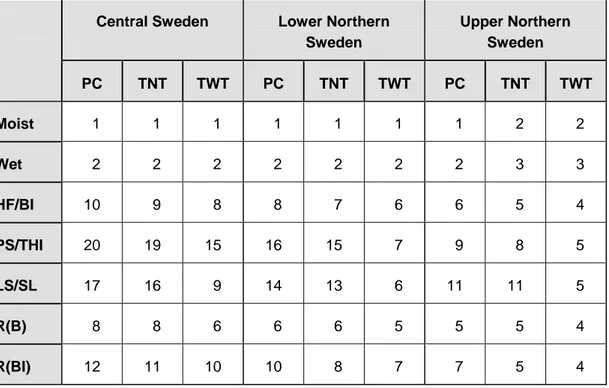
The results for the speed reductions are shown in Tables 1 to 3. The data from all sites are aggregated and generalized to ensure more reliable and consistent results. In the tables, the reductions are related to 1: the climate zones, 2: salted or unsalted roads, and 3: the width of the roads, in two categories. Thus, the results may be used under different assumptions.
The speed reductions are expressed as percentages of the speed at dry, bare roadway.
Table 1 The Decrease in Speed for Different Road Conditions and Different
Climate Zones, Relative to Dry, Bare Roadway.
Central Sweden Lower Northern
Sweden Upper Northern Sweden PC TNT TWT PC TNT TWT PC TNT TWT Moist 1 1 1 1 1 1 1 2 2 Wet 2 2 2 2 2 2 2 3 3 HF/BI 10 9 8 8 7 6 6 5 4 PS/THI 20 19 15 16 15 7 9 8 5 LS/SL 17 16 9 14 13 6 11 11 5 R(B) 8 8 6 6 6 5 5 5 4 R(BI) 12 11 10 10 8 7 7 5 4
Table 2 The Decrease in Speed for Different Road Conditions on Salted and
Unsalted Roads, Relative to Dry, Bare Roadway.
Salted Roads Unsalted Roads
PC TNT TWT PC TNT TWT Moist 1 1 1 3 3 3 Wet 2 2 2 4 4 4 HF/BI 9 8 8 6 5 5 PS/THI 19 18 16 12 12 10 LS/SL 16 15 10 11 11 7 R(B) 7 7 5 5 5 4 R(BI) 11 9 9 7 6 5
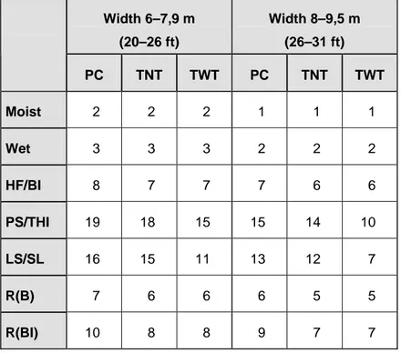
Table 3 The Decrease in Speed for Different Road Conditions on Roads with
Different Widths, Relative to Dry, Bare Roadway.
Width 6–7,9 m (20–26 ft) Width 8–9,5 m (26–31 ft) PC TNT TWT PC TNT TWT Moist 2 2 2 1 1 1 Wet 3 3 3 2 2 2 HF/BI 8 7 7 7 6 6 PS/THI 19 18 15 15 14 10 LS/SL 16 15 11 13 12 7 R(B) 7 6 6 6 5 5 R(BI) 10 8 8 9 7 7
1.9
The accident risk model
The underlying hypotheses for the accident risk model are: the risk is varying between the different ice and snow road conditions specified above; also, it differs between the climate zones of Sweden, because the more common wintry conditions are, the better drivers adapt to the situation. A subsequent hypothesis is that the less duration a certain ice or snow condition has throughout the winter season, the higher is the risk, Wallman (6).
Another hypothesis is that the accident rate is higher for early and late parts of the winter, compared to the rate for the mid-winter, Bergström (7).
To estimate the accident rate in a specific ice or snow condition for a certain road network, two data must be known: the number of accidents in the road condition in question, and the vehicle mileage in that condition. There is a major problem in collecting data for the vehicle mileage, the duration of icy and snowy conditions is often very short, which calls for close observations of the road network throughout the winter season.
1.10 Data
Capture
The SNRA monitored the roadway condition all over Sweden in the four winter seasons of 1993–1994 to 1996–1997. The intention was to check the performance of the winter maintenance contractors. The observations were made at about 2,000 sites on the national road network with a frequency of about one observation per site and week. From this data it was possible to estimate the distributions of the different roadway conditions under the four winter seasons. Roadway condition data were aggregated for road networks: grouped into the four climate zones, and
into the different standard levels of operation. Finally, the vehicle mileage in each roadway condition could be estimated.
The accidents reported by the police during the four winter seasons were used, grouped into the reported roadway condition at the accident. The accidents were linked to the same road networks as the roadway conditions.
1.11 Results
The average accident rates vary between the different ice and snow conditions and between the climate zones, as was stated in the first two hypotheses. However, the differences between the climate zones also apply for the rate for dry, bare roadway. An explanation for this could be that the extents of police reports vary between the climate zones; e.g. Upper Northern Sweden is very sparsely populated, one may suspect that the police have difficulties in traveling many miles for reporting a distant, minor accident.
As an example, the accident rates for the salted and unsalted road networks in Central Sweden are displayed in Figure 3.
Central Sweden, Accident Rates at Different Road Conditions 1993/94 - 1996/97 0,0 0,5 1,0 1,5 2,0 2,5 3,0 3,5 4,0 4,5
Salted roads Unsalted roads
Dry bare ground Wet bare ground Hard-packed snow Black ice Loose snow
Accident rate
Figure 3 Average accident rates (accidents per million vehicle kilometers) at
different road conditions, salted and unsalted roads.
The accident rates for ice and snow conditions are much larger for the salted network and still larger if the rates are related to the rate at dry, bare ground. For example, black ice is 16 times more dangerous on salted roads, but “only” about 6 times on unsalted roads.
An interesting question is whether the accident risk always is the same for each ice and snow condition, or if the risk varies with the duration of the conditions (the third hypothesis mentioned above).
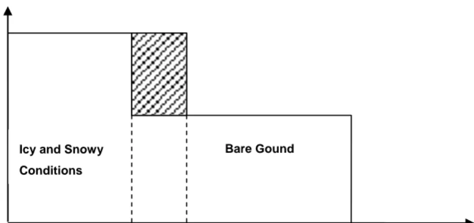
Assume that the accident rate has two levels, one for ice and snow and another for bare ground conditions. Some part of the vehicle mileage during the winter
season runs on ice and snow, and some runs on bare ground. What will happen if the maintenance effort is improved?
Accident Rate
Bare Gound Icy and Snowy
Conditions
Vehicle Mileage during the Winter Season
Figure 4 The optimistic model.
Accidentrate
Figure 5 The pessimistic model.
The striped area in Figure 4 shows the effect of improved maintenance. The vehicle mileage is decreased on ice and snow. The optimistic model states that the accidents decrease by a number, corresponding to the area of the striped square. On the other hand, the accident rate on ice and snow may increase, because drivers will have fewer occasions and less time for adapting their driving behavior
Vehicle mileage during the winter season
Icyand snowy
Bare ground conditions
to icy and snowy conditions. If this is the case, the accidents increase on ice and snow corresponding to the striped area in Figure 5.
A possible hypothesis is that improved maintenance will result in fewer accidents, but not to the full extent like in Figure 3.
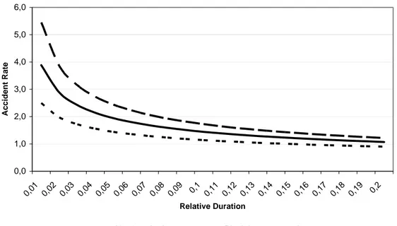
For testing this hypothesis, the same set of data as before can be used. The result shows an exponential relation between the accident rate and the duration for each of the three different ice and snow conditions. Like the average accident rates, this result varies between the climate zones. Figure 6 displays the result from Central Sweden.
Accident Rate, Climate Zone Central Sweden
0,0 1,0 2,0 3,0 4,0 5,0 6,0 0,01 0,02 0,03 0,0 4 0,0 5 0,06 0,07 0,08 0,09 0, 1 0,11 0,12 0,13 0,14 0,15 0,1 6 0,17 0,18 0,19 0, 2 Relative Duration Ac c ide nt Ra te
Hard-packed snow Black ice Loose snow
Figure 6 The accident rate (accidents per million vehicle kilometers) as a
function of relative duration for three ice and snow conditions.
The relative duration denotes the vehicle mileage on the particular ice and snow condition related to the total vehicle mileage throughout the winter season. Roughly, the number 0.01 corresponds to the duration of about 2 days of the winter season.
If the accident rate functions are related to the rate at dry, bare conditions, the relations are found to be valid for all climate zones. In Figure 7, the relative accident rates are shown, valid for whole Sweden.
Accident Rate Relative to Dry, Bare Road, Entire Sw eden 0 5 10 15 20 25 30 35 40 0,01 0,02 0,03 0,04 0,05 0,06 0,07 0,08 0,09 0, 1 0,11 0,12 0,13 0,14 0,15 0,16 0,17 0,18 0,19 0, 2 Relative Duration R elat ive A cci d en t R at e
Hard Packed Snow Black Ice Loose Snow
Figure 7 The relative accident rate (relative to the rate at dry, bare road) as a
function of relative duration for three ice and snow conditions.
The fourth hypothesis, if the accident rates at early and late winter periods are larger than that for the mid-winter, was tested by assessing accident rates for early and late winter periods, with varying length, 2, 3, and 4 weeks respectively. Generally, the results show considerably increased accident rates at early as well as late winter periods, and the earlier and later, the higher the rates. However, the variations were so large between the climate zones and between the different road conditions that no average values seem to be relevant.
1.12 Acknowledgement
The development of the Winter Model is co-financed by the National Swedish Road Administration (SNRA), and the Swedish Agency for Innovation Systems (VINNOVA).
1.13 References
1. Vägverket (Swedish Road Administration). Drift 96: Allmän teknisk
beskrivning av driftstandard. Publ.1996:16. Vägverket. Borlänge. 1996.
2. Vägverket (Swedish Road Administration). Operation 94: General
Techni-cal Description of Operation Service Levels. Publ.1994:100. Vägverket.
Borlänge. 1994.
3. Vägverket (Swedish Road Administration). Vinter 2003: Val av
vinterväg-hållningsstandard. VV Publ. 2002:147. Vägverket. Borlänge. 2002.
4. Wallman, C.G. Vehicle Speed and Flow in Various Winter Road Conditions. In Proceedings of the Ninth Maintenance Management Conference, TRB, Conference Proceedings 23, Washington, D.C., 2001, pp 159–166.
5. Wiklund, M. Pair Comparing Method. VTI rapport 495A. VTI. Linköping. 2003.
6. Wallman, C.G. Tema Vintermodell: Olycksrisker vid olika väglag. VTI notat 60-2001. VTI. Linköping. 2001.
7. Bergström, A. Tema Vintermodell: Olycksrisker under för-, hög- och
2
Winter Road Condition Model
2.1 Abstract
The large-scale project, the Winter Model, will result in a model for assessing the most important effects and their monetary value of changes of winter maintenance strategies and operations.
The winter road condition model is the central part of the Winter Model. The road condition model will characterize the state of a winter in terms of a road condition description hour by hour. The road condition model provides input data for the other models where different effects such as accident risk, travel time, fuel consumption, and environmental effects are assessed.
In the first stage we intend to develop a model that describes how road conditions are affected by weather, maintenance measures taken and traffic on two lane rural roads with a width of 7 to 9 m and speed limit of 90 km/h.
To a great extent, the basis for developing the winter road condition model will be data already collected from nine observation sites with the purpose of developing the accessibility model.
For several periods data from these observation sites contain information hour by hour regarding weather, traffic flow, initial road condition, maintenance measures taken and specified types of road condition development mainly connected with snow ploughing and anti-icing measures. Additional information, mostly development of ruts down to the pavement in hard-packed snow or thick ice caused by vehicles with studded tyres, and conditions for a wet or moist road to dry out will be collected by field studies as from the winter season 2002–2003.
2.2 Background
The large-scale project, the Winter Model, will result in a model for assessing the most important effects and their monetary value of changes of winter maintenance strategies and operations. The effects are assessed for road users, road administrators and environment.
Four papers will be presented at this symposium treating different parts of the model: in this paper the Winter Road Condition Model will be presented. Another paper deals with the Accessibility and the Accident Risk Models, and finally, two papers deal with the Environmental Model.
The winter road condition model is the central part of the Winter Model. The model will characterize the state of a winter in terms of a road condition description hour by hour. The road condition model provides input data for the other models where different effects such as accident risk, travel time, fuel consumption, and environmental effects are assessed. The model is limited to describing winter road conditions on two lane rural roads.
2.3 Model
development
In the first stage we intend to develop a model that describes how road conditions are affected by weather, maintenance measures taken and traffic on a road with a width of 7 to 9 m and speed limit of 90 km/h. The model is limited to four cases concerning winter maintenance standard classes and traffic flow. See Table 1. Standard class A3 is the second lowest class of salted roads and standard class B1 is the highest class of non-salted roads, “Drift 96. Väglagstjänster” (1).
Table 1 Four Cases for the Road Condition Model.
Winter maintenance standard class Traffic flow (AADT) A3 1,500 3,000 B1 1,000 3,000
To a great extent, the basis for developing the winter road condition model will be data already collected from the nine observation sites, during one or two winter seasons, with the purpose of developing the accessibility model.
The observation sites represent the following variation.
• Climate zone: Central, lower northern and upper northern Sweden. • Standard class: A3, A4 and B1.
• Traffic flow: AADT 1,500 to 3,500. • Road width: 6.5 to 9.2 m.
• Speed limit: 90 and 110 km/h.
For several periods data from these observation sites contain information hour by hour regarding weather, traffic flow, initial road condition and maintenance measures taken. Also specified types of road condition development – mainly connected with snow ploughing and anti-icing treatment – can be studied. Additional information will be collected in special field surveys as from the winter 2002–2003. One survey will cover the development of ruts down to the pavement in hard-packed snow or thick ice caused by vehicles with studded tyres. Also the mechanism for a wet or moist road to dry out will be studied.
2.4
Winter road condition model, structure
The first version of the road condition model will be constructed according to the following outline. The road condition will be described for each of five strips of the lane, “Metodbeskrivning 105:1996. Bedömning av vinterväglag” (2). In Figure 1 half a carriageway is shown.
Lane
Shoulder
Ditch
1 2 3 4 5 1 = Edge of lane. 2 = Right wheel track. 3 = Between wheel tracks. 4 = Left wheel track.5 = Middle of the carriageway.
Figure 1 Lane divided into five strips.
Starting from the centre of the road, we can see the lane, the shoulder and the ditch. Snow is covering the road except in wheel tracks. The lane is divided into the following strips:
• Edge of lane. • Right wheel track. • Between wheel tracks. • Left wheel track.
• Middle of the carriageway.
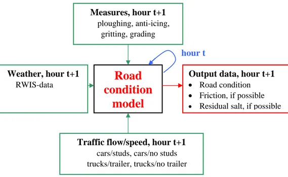
Measures, hour t+1 ploughing, anti-icing,
gritting, grading
Figure 2 Input and output data to and from the road condition model.
Input data
• Road condition during the hour t (a 60 minute period) for each of five strips of the lane.
• Amount of residual salt on the carriageway during the hour t, if possible. • Weather from the Road Weather Information System during the hour t+1.
Weather includes air temperature, road surface temperature, dew point temperature, type and amount of precipitation, wind speed and weather situation. Examples of weather situations are snowfall, rain, blowing snow and risk of slippery surfaces due to for example frost formation on a cold carriageway.
• Traffic flow and average speed during the hour t+1. Data are divided into cars using studded tires, cars not using studded tires, trucks with a trailer and trucks with no trailer.
• Maintenance measures taken during the hour t+1. These data are divided into snow ploughing, icing treatment, snow ploughing combined with anti-icing treatment, gritting and grading.
Output data
• Road condition during the hour t+1 for each of five strips of the lane.
• Road condition during the hour t+1 at an aggregated level. For example the following five types of road condition: Dry bare ground, moist/wet bare ground, hard-packed snow/thick ice, black ice/hoar-frost and loose snow/slush.
• Friction class in wheel tracks during the hour t+1, if possible.
• Amount of residual salt on the carriageway during the hour t+1, if possible.
Road
condition
model
Output data, hour t+1 • Road condition • Friction, if possible
• Residual salt, if possible
hour t
Weather, hour t+1 RWIS-data
Traffic flow/speed, hour t+1 cars/studs, cars/no studs trucks/trailer, trucks/no trailer
2.5
First attempt at a winter road condition model
As a basis for developing and testing the computer program which will manage input and output data and make calculations in the Winter Model a first model attempt is designed. The attempt consists of three sub models:
1. One for a wet or moist road to dry out. 2. One for anti-icing treatment.
3. One for snow ploughing combined with anti-icing treatment.
The sub models are still to a great extent intuitive and without accurate empirical foundation but contain some realistic relationships between different variables.
We use the following notation of the concept of time. See Figure 3.
o’clock t t+1 t+2 t+3 t+4 t+5 │ │ │ │ │ │
hour t t+1 t+2 t+3 t+4
Figure 3 Notation of the concept of time.
• t o’clock is an instant. For example 10 o’clock, 11 o’clock etc.
• The hour t is a period of 60 minutes immediately after t o’clock. For example the hour 10 means the time period 10.00 to 10.59.
2.6
Sub Model: Drying
2.6.1 Assumptions and Prerequisites
If the amount of water on the road is: • 50 g/m2
the road condition is wetbare ground. • 50–5 g/m2
the road condition is moist bare ground. • < 5 g/m2
the road condition is dry bare ground.
1 mm of rain ↔ the amount of water on each m2 of the road = 100x100x0.1 =
1,000 cm3/m2 = 1,000 g/m2.
If the amount of water on the road is > 50 g/m2 we assume that the amount of water is halved each time the traffic flow runs up to 100 pbekv.
Definition: pbekv = (the number of cars)x1 + (the number of trucks with no
trailer)x3 + (the number of trucks with a trailer)x7.
If the amount of water on the road is ≤ 50 g/m2 it is assumed that drying depends on dew point temperature, road surface temperature and traffic flow. Also wind speed and wind direction are important parameters which will be included when empirical data are studied more closely.
2.7
Sub Model: Anti-Icing Treatment with Salt
2.7.1 Assumptions and Prerequisites
It is assumed that anti-icing treatment is carried out with brine and that a salting pass takes 2 hours.
If icy conditions are indicated during hour t, action is ordered at t+1 o’clock. After the driver has reported for duty and the vehicle has been made ready, which takes 1 hour, action on the road begins at t+2 o’clock and is carried out during hours t+2 and t+3. This means that, as an average for the salting pass, salting is
performed at t+3 o’clock. The change in road conditions as a result of salting, as an average for the salting pass, shall then refer to t+3 o’clock.
2.7.2 Model Attempt
The relationship between weather (HF=risk of hoar frost), activity (D+V=time for driver to report for duty and for the vehicle to be made ready, S=salting), time of salting as an average for the pass (↑) and simplified description of road condition, is set out in Figure 4 below. DB=dry bare ground,MB=moist bare ground.
o’clock t t+1 t+2 t+3 t+4 t+5 Hour │ t │ t+1 │ t+2 │ t+3 │ t+4 │
Weather │ HF │ HF │ HF │ – │ – │
Activity │ – │D+V│ S │ S │ – │
Ave. time for pass ↑
Road condition │ DB │ DB │ DB │ MB │drying
Figure 4 Model attempt for anti-icing treatment with salt.
If slippery conditions persist, another salting pass must be carried out. When this is done depends on the type of slippery conditions in question.
2.8
Sub Model: Snow Ploughing combined with
Anti-Icing Treatment
2.8.1 Assumptions and Prerequisites
It is assumed that snow falls over 5 to 7 hours and provides moderate amounts of snow, i.e. 2 to 4 cm loose snow, and that only two passes of combined action are needed. Each pass takes 6 hours. It is also assumed that a separate anti-icing treatment with moist salt is performed before the snowfall. Such an action is assumed to require 2 hours.
If the first snowfall is indicated during hour t1, salting is carried out during the
hours t1-2 and t1-1. This means that the change in road conditions, as an average
for the salting pass before the snowfall, should refer to t1-1 o’clock.
Combined action begins when ≥1 cm snow has fallen, aggregated by the hour. This is assumed to have occurred at t2 o’clock. The first pass is then run during the
hours t2 to t2+5. This means that the change in road conditions, as an average for
the first pass of snow ploughing combined with anti-icing treatment, should refer to t2+3 o’clock.
The second pass with combined action begins 6 hours after the start of the first pass, i.e. at t2+6 o’clock. The change in road conditions as an average for the second pass should then refer to t2+9 o’clock.
2.8.2 Model Attempt
The relationship between weather (S= snowfall), amount of snow in cm per hour, activities (S=salting, CA1 and CA2 =combined action of the first and second pass
respectively), time of salting and combined action as an average for the pass (↑) and simplified description of road conditions, is set out in Figure 5 below. DB=dry bare ground, MB=moist bare ground, WB=wet bare ground, SL=slush,
o’clock t1-2 t1-1 t1 t1+1 t2 t2+1 t2+2 t2+3 t2+4 t2+5 t2+6
Hour │ t1-2 │ t1-1 │ t1 │ t1+1 │ t2 │ t2+1 │ t2+2 │ t2+3 │ t2+4 │ t2+5 │ t2+6 │
Weather │ – │ – │ S │ S │ S │ S │ S │ S │ S │ – │ – │
Amt. of snow │ – │ – │ 0.4 │ 0.8 │ 0.6 │ 0.8 │ 0.3 │ 0.5 │ 0.3 │ – │ – │
Activity │ S │ S │ – │ – │ CA1 │ CA1 │ CA1 │ CA1 │ CA1 │ CA1 │ CA2 │
Ave. time for pass ↑ salt ↑ comb. action 1
Road condition │ DB │ MB│SL/LS│SL/LS│SL/LS│SL/LS│SL/LS│ SL │ SL │ SL │WB/SL│
Figure 5 Model attempt for snow ploughing combined with anti-icing treatment
with salt.
2.9
Measurement of rut development
At the end of January 2003 an attempt was made to measure rut development in hard packed snow/thick ice caused by vehicles with studded tyres. The measure-ment site was situated in upper northern Sweden. The road was covered by ice ~1 cm thick.
Development of ruts down to the pavement was examined using a special device, ”Primal”. See Figures 6 and 7 below.
Figure 7 Primal towards the end point (by the stand) on the shoulder.
“Primal” is a small self-propelled device, developed by VTI. It is normally used for measuring cross sections of paved roads in the summer. It is located at the starting point and aimed at the end point for the measurement. Then it travels across the road and measures the level of the surface on to the end point. The starting point/end point is a nail with a washer driven into the pavement. In this case the road condition is 1 centimetre of thick ice. The precision of the measurement is very good. A cross section measured by “Primal” is shown in Figure 8.
2003-01-27, cross section no 8 -5 0 5 10 15 20 0 1 2 3 4 5 Length (m) Height (mm)
Figure 8 Cross section measured by Primal.
A reference plane is defined by the starting point and the end point and the cross section is drawn in relation to the reference plane. We can see the starting point (the nail in the pavement), 1 centimetre of thick ice on the pavement, left wheel track, between wheel tracks, right wheel track, shoulder and down from the thick ice to the end point (the second nail).
A total of 38 cross sections were measured over four days. By plotting these in the same diagram, the gradual development of ruts would be shown. Unfortunately, we had problems with data collection, which meant that rut development could not be evaluated in this simple way. Average cross sections from Days 1 and 4 were instead produced by manual methods. The results are plotted in Figure 9.
Figure 9 Average cross sections from day 1 (light curve) and day 4 (dark curve)
superimposed upon each other.
It was estimated that the ruts deepened by max. 1 mm between the first and last measuring event, i.e. over about three days. Owing to the manual method, there is naturally quite a large uncertainty in this estimate. During the same period about 2,000 cars with studded tyres, which abraded the thick ice, travelled over the road. The relative wear in the middle of the wheel track in thick ice can then be estimated as 1.0/2000 = 0.0005 mm/car with studded tyres.
In the present case, this would mean that the ca 1cm thick ice would be worn away in the middle of the wheel track after ~20,000 cars with studded tyres have passed. This represents traffic during approximately one month.
2.10 Acknowledgments
The Winter Model project is co-financed by the Swedish National Road Administration and the Swedish Agency for Innovation Systems. The financial support is gratefully acknowledged.
2.11 References
1. Vägverket (Swedish Road Administration). Drift 96. Allmän teknisk
be-skrivning av driftstandard. Publikation 1996:16. Vägverket. Borlänge,.
1996.
2. Vägverket (Swedish Road Administration). Metodbeskrivning 105:1996.
Bedömning av vinterväglag. Publikation 1996:59. Vägverket. Borlänge.
3
Patterns of Residual Salt on Road Surface –
Case study
3.1 Abstract
A field study was performed in order to investigate the patterns of residual salt on a road surface and the mechanisms involved in transporting the salt off the road into the roadsides. The residual salt was measured in nine segments across a road and repeated in 2–24 hour intervals, depending on the road surface conditions. The results will be implemented in a winter maintenance management model under development by the Swedish National Road and Transport Research Institute (VTI). The results showed clearly that the vehicles are important for redistribution of the salt from the wheel paths. A light snowfall increased the salt content in the roadway, probably because of redistribution of salt from outside the road border lines by passing vehicles due to increased wetness. The amount of residual salt in the wheel paths could be modeled rather well using an exponential function, where the amount of salt was depending on the accumulated number of vehicles after each salting occasion. A model constant was suggested to be related to the road surface conditions.
3.2 Introduction
Salt (mainly sodium chloride) is widely used in winter maintenance for deicing and anti icing purposes. Because of the well known environmental draw-backs of salt exposure to roadside vegetation and groundwater, the road keepers constantly strive to minimize the amount of salt used during the winters. In that context, knowledge of the content of residual salt remaining on the road surface is of great importance for the tactical decisions of whether or not another salting action is needed. The salt remaining on the road surface will also, sooner or later, be transported off the road by different means and, hence, expose the roadside to different amounts of salt. At the Swedish National Road and Transport Research Institute (VTI) a winter maintenance management system (The Winter Model – WMMS) is under development. The Winter Model consists of sub models for assessing the state of the road, its effects and their appraisement (see paper by Wallman, in this proceedings). One of the sub models is describing the environmental effects by modeling the roadside exposure to salt (see paper by Gustafsson & Blomqvist, in this proceedings). In order to model the roadside exposure to salt, knowledge of the amount of residual salt available on the road surface is a prerequisite. The purposes of the field studies described in this paper is to gather field data of the pattern of residual salt on the road surface together with information of the factors influencing the transport of the salt off the road. In this paper these patterns and relationships are discussed in relation to how this knowledge should be used within the Winter Model. Also, a modeling approach to describe the decline of residual salt is made.
3.3 Residual
salt
While there are numerous investigations performed on the environmental effects of deicing salt exposure to the roadsides, investigations of the mechanisms responsible for the transport of salt from the roads to the surroundings, are rather rare.
In a Danish investigation, the amount of residual salt after a salting occasion was shown to be linearly related to the number of vehicle passages after the salting, at least when the traffic intensity was between 2,500 to 3,500 vehicles per day (1). The traffic intensity explained in the best cases 17 to 18% of the varia-tion. In two of the four roads that were investigated the same relation between the residual salt and the traffic intensity could not be found. This was suggested to be explained by the relationship maybe not being linear (1).
In a Swedish investigation, the residual salt decline showed to be exponentially related to time (2). A model was designed with the presumption that the salt only will leave the road surface by the transportation of liquids off the road. Another presumption was that the total amount of salt across the road surface only can stay at a constant level or decline by time (unless another salting action is taken). Locally, however, the residual salt may increase initially during precipitation due to relocation of salt from the road center and other less trafficked areas.
3.4 Field
work
The residual salt was measured by a chlorine meter (SOBO20, see Figure 1). This instrument works by splashing a precise volume of measuring liquid (15% acetone) on an exact delimited road surface area. The electric conductivity and temperature are measured in the liquid and thereby the amount of NaCl per square meter can be calculated. The measurements were separated by on what section of the transect it was made. The road was divided into nine segments from one edge of the road to the other; road edge (outside the white line), in the right wheel path, in between the wheel paths, in the left wheel path, at the road center, in the left wheel path, in between the wheel paths, in the right wheel path, and, finally, the other road edge. Each measurement in the study is the mean value of three individual measurements, next to each other (see Figure 1). For each new measurement the three points were chosen next to the earlier measurement but shifted slightly towards the direction where traffic comes from, in order to avoid influence from the acetone solution already flushed out on the road surface. A similar procedure was taken in a Danish investigation using the same measuring equipment (1).
Two field sites were used to collect the data needed. At the first place, Vimmerby, an existing standard road weather information system (RWIS) was used to gather data on the traffic amount and type on an hourly basis. The traffic counter was installed in the pavement and the traffic data was collected by magnetic induction. At the other field site, Klockrike, the traffic data was collected by a rubber tube, which needed to be disconnected when the plowing truck was passing the field site. The traffic data, salting occasions and mean values of the residual salt in the left wheel tracks are presented in Figure 2. The traffic data is calculated as the sum of the number of private cars, heavy trucks times 5, buses times 5 and heavy trucks with trailers times 7. The coefficients of 5 and 7 are not evaluated in this paper. The posted speed limits were 90 km h-1 at both field sites.
Figure 1 Measuring the residual salt on the road surface – note how the road
surface is divided into segments: a) road edge, b) wheel track, c) in between wheel tracks, d) wheel track and e) road centre. The measurements continue on the other half of the road.
0 2 4 6 8 10 12 14 16 R e si du al s a lt i n lef t whe e lt ra c k ( g m
-2) Residual salt in wheeltracks Deicing action 0 100 200 300 400 500 feb-08 feb-09 feb-10 feb-11 feb-12 feb-13 feb-14 feb-15 feb-16 feb-17 feb-18 feb-19 feb-20 feb-21 feb-22 feb-23 feb-24 feb-25 feb-26 feb-27 feb-28 mar-01 mar-02 mar-03 mar-04 mar-05 mar-06 mar-07 mar-08 N u mb e r of c ar s p er ho ur
Private car equivalents
Figure 2 Residual salt in the wheel tracks, deicing actions and traffic data.
Traffic data is missing for the first nine days. For that period the data used (dashed line) are compiled by the mean hourly data for the consecutive two weeks.
3.5
Results and discussion
The residual salt transects of the first 288 hours of measurements at Klockrike field site are compiled in Figure 3, where the mean values of the residual salt amount in each segment of the road transect is presented along the vertical axis. The different repeated measurements are shifted along the horizontal time-axis. The “space-time”-graph is then produced by linear triangulation of the data points. It can be seen that the amount of salt on the roadway, on the pavement inside the white lines of the road edges, is quite low for the first couple of days, but that there seem to be high amounts of salt gathered on the road surface outside of the white lines. For the first 18 hours there also seem to be some salt remaining on the road surface from the salting occasion that took place in the morning of the 8th of February (i.e. 72 hours earlier). Usually the decline of the amount of residual salt on the road surface works faster than this, but one should bear in mind the fact that the road surface conditions were dry to moist, (i.e. with very low degree of wetness). These rather dry road conditions prevailed during the larger part of the investigation period that is illustrated in Figure 3.
There are two exceptions when the road surface got wetter because of a light snowfall. The first period is during 13th February and the second is during the 15th of February. These snowfalls are marked with a small “snowflake” in Figure 3 at each time of their observation. What can be seen as an effect of the higher degree of wetness of the road surface is an increase of residual salt starting in hour 66 and peaking in hour 72, especially in between the wheel paths in each direction of the road (see Figure 3). This is suggested to be explained by redistribution of salt accumulated on the pavement outside of the roadway into the driving lanes by passing vehicles. Similar effects have been discussed by Ericsson and Gustavsson (2). The first salting action, after February 8th, was taken in the morning of February 15th, which can be seen as a major increase in the amount of residual salt. The salting is repeated in the morning of the 17th of February.
During the latter half of the period illustrated in Figure 3, it becomes very evident that the salt is gathering between the wheel tracks and in between the road halves. The standard deviation of a transect across the road is approximately twice as high (during February 20th) as compared to the standard deviation of a 24-hour time window during the same period (see Figure 4). The usefulness of residual salt measurements has sometimes been questioned. This study, however, shows that, as long as one really is doing the repeated measurements within the same segment of the road, it is more likely to get a similar value several hours later, than if moving to another segment of the road right after the first measurement.
Figure 3 The development of residual salt pattern by time. X-axis is a time-scale
with the number of hours from start denoted on the lower axis and the dates on the top axis. The Y-axis is a transect across the road with each measurement in time and space marked as a black dot. Two periods of very light snowfall is marked by small “snowflakes” on the top axis.
0 1 2 3 4 5 6 228 234 240 246 252 Time (h) S tan dar d dev iat ion ( g m -2) Transect Road edge W heel track between wheels W heel track Road centre W heel track between wheels W heel track Road edge
Figure 4 The standard deviation of the residual salt measurements in the transect
across the road and in a ”time window” of twenty four hours in each type segment: road edges, wheel tracks and between the wheels and in the road center. For the modeling purposes in this study the two inner wheel tracks (closest to the road center) have been chosen to represent the amount of residual salt on the road surface available to roadside exposure. The reason for using the two inner wheel tracks in this first phase of modeling is that it is thought that this is the track that both private cars and larger heavy vehicles most often share, and that the other two wheel tracks are more scattered in space. The mean value of the residual salt measurements in the two inner tracks is presented in Figure 2. In order to find out the rate at which the salt is leaving the road (or redistributed on the road) and
since the pattern of salt distribution on the road seem to be strongly correlated to the traffic, a model (function 1) is tested that uses the salt application as a start value and the accumulated traffic after the salt application as the factor influencing the rate at which the salt is leaving the wheel tracks. Testing equation 1, where k is the rate by which the salt leaves the wheel track, using field data collected in Klockrike from the salting occasion in February 19th to the salting occasion in February 22nd, gave the result that can be seen in Figure 5.
eqacc PC
S
RS
=
⋅
e
−k⋅ (Eq. 1) where RS = residual salt S = salt usePCeqacc = accumulated private cars equivalents
y = 13,854e-0,153x R2 = 0,7819 y = 12,689e-0,2027x R2 = 0,8729 0 2 4 6 8 10 12 14 0 2 4 6 8 10 12
Accumulated traffic (number of thousand private car equivalents)
R e s id ual s alt in lef t w he el tr ac k s ( g m -2) Vimmerby Klockrike
Figure 5 The relation between traffic and amount of residual salt in the wheel
tracks in the two field sites Vimmerby and Klockrike.
This model suggests that the salt amount after the salting action in the morning of February 19th is 12.689 g m-2 and that the coefficient k describing the decrease is -0.2027. Letting k, calculated from three consecutive days during the field experiment, represent the conditions during the entire 25-day long field period gave the modeling results that can be seen in Figure 6. With exception of the two occasions when the light snowfall caused a suggested redistribution of the salt on the road (February 13th and 15th); the model describes the residual salt surprisingly well until February 27th. A reason for the good fit of the model to the measured
data may be the fact that the weather situation during the investigation period was rather stable.
A value of the coefficient k was also calculated from the field data collected in the Vimmerby site (also seen in Figure 5). The Vimmerby k-value differs somewhat from the Klockrike k-value, implying a somewhat slower rate of residual salt decrease in Vimmerby. Whether this is a result of different wetness of the road surface during that time period, different road surface characteristics, a different composition of the traffic, or the use of another winter maintenance equipment in Vimmerby is however not yet known to us.
0 2 4 6 8 10 12 14 16 18 20 feb 8 feb 9 feb 10 feb 11 feb 12 feb 13 feb 14 feb 15 feb 16 feb 17 feb 18 feb 19 feb 20 feb 21 feb 22 feb 23 feb 24 feb 25 feb 26 feb 27 feb 28 mar 1 mar 2 mar 3 mar 4 mar 5 mar 6 mar 7 mar 8 R es idual s al t ( g m -2) Residual salt Deicing action Model
Figure 6 Modeling results as compared to the field measurements of the residual salt and the deicing actions taken.
Implementation in the Winter Model requires calibration of the model using data from field investigations under various conditions regarding the weather, traffic and salting. Also, in order to be able to create a more generic model, different sites should be used, representing different pavements and different traffic compositions.
Issues that need to be addressed during the field investigations during the 2003–2004 and 2004–2005 winter seasons are:
• What is the correct relation between a private car, a bus, a truck and a truck with trailer, regarding their potential to force the salt solution and salt laden slush off the road surface into the surroundings?
• What is the influence of the different road surface states on the ability of the vehicles to force the salt off the road?
• How do climatic factors as i.e. local wind speed and precipitation influence the decline of residual salt?
• How shall salt re-distribution on the road surface be modeled?
3.6 Acknowledgements
This study was made as part of the project ”Winter Model” which is performed at the Swedish National Road and Transport Research Institute (VTI) and is financed by the Swedish Road Administration and the Swedish Agency for Innovation Systems.
3.7 References
1. Fonnesbech, J.K. & Prahl, K.B. Saltlagespredning på trafikveje, Fyns Amt, Denmark, April 2000. (In Danish). http://www.fyns-amt.dk/wm103165
Accessed Dec. 1, 2003.
2. Ericsson, B. & Gustavsson, T. Projekt Restsalt – Empirisk datormodell för
beräkning av restsalt, vätskefilm och fryspunkt. Bergab
4
Modeling Exposure of Roadside Environment
to Airborne Salt – Case Study
4.1 Abstract
A field study was performed in order to investigate the relationships between the salt use, the mechanisms affecting the salt emission, dispersion and the salt exposure in a modeling approach. The salt was collected on gauze filter salt vanes at distances of 2.5 m to 100 m from the road, allowing a time resolution of 30 minutes to 24 hour exposure time. The results will be implemented in a winter maintenance management model under development by the Swedish National Road and Transport Research Institute (VTI). The results showed that the roadside exposure to airborne salt is strongly related to the wind direction. The road conditions of packed snow and thin ice seemed to temporarily abate the roadside exposure by capturing the salt on the road surface. Even at a distance of 100 m from the road a positive relation of the wind sum and chloride deposition showed on days with strong winds. The modeling approach indicate the importance of residual salt, traffic, road surface characteristics, and wind for roadside exposure but also that there are several aspects of these variables that need further investigations.
4.2 Background
Salt has been widely used for decades in order to maintain road safety and accessibility of the road network at acceptable levels also during the winter season. The use of sodium chloride for deicing and anti icing purposes started in the 1940’s in the United States and has increased ever since, as the motoring has developed (1). In the Nordic countries the use of deicing salt started in the mid-1960. Already at an early stage, it was recognized that the use of salt had not only the desired effect of improved traffic safety and accessibility but also several negative impacts. Numerous investigations of impacts on e.g. vegetation, soil and groundwater have been presented and the matter is still of great concern in North America, Europe and Japan. Recent studies made in Sweden have been studying the problem in relation to damage to roadside vegetation (2) and in relation to damage to ground water aquifers (3).
The transport of salt from the road to the roadside environment is the main environmental concern of winter maintenance. The basic mechanisms determining the salt exposure are salt dose to the road, road conditions, traffic characteristics (type, intensity and speed) and meteorological parameters, such as wind. Salt use is the origin of salt exposure and naturally affects the deposition in the roadside environment. Salt use in combination with wind can result in the kind of patterns seen in Figure 1 (4). The deposition follows the salt use and the lee side of the road receives markedly higher amounts of salt than the upwind side. The importance of wind as the main transport mechanism was shown by Blomqvist (4) by studying the percentage of winds with a road perpendicular wind component towards the road in relation to the percentage of chloride deposition into containers placed on the downwind side of the road (see Figure 2). The correlation was good especially when the wind was almost exclusively blowing from one side. In between these extremes the divergence is somewhat larger.
0 5 10 15 20 25 30 1 2 3 4 5 6 7 8 9 Investigation period N u m b er o f sal ti n g o c casi o n s 0 250 500 750 1000 1250 1500 D ep o si ti o n at 14 m ( m g C l m -2 )
Figure 1 Relation between the salt use and the deposited amount of chloride on
the southeastern (triangles) and northwestern (squares) side of the road, at 14 m distance during the nine investigated periods (4).
0% 10% 20% 30% 40% 50% 60% 70% 80% 90% 100% 0% 10% 20% 30% 40% 50% 60% 70% 80% 90% 100%
Winds with NW-component
P e rc e n ta ge C l d e po s it e d o n S E si d e o f t h e r o ad
Figure 2 Percentage of Cl deposited on the south-eastern side of the road as
related to the percentage of winds with a NW-component. (□ = 12 m, * = 20 m, ♦ = 14 m) (4).
Few investigations have related the roadside salt exposure to the deicing action itself, to the road-surface and traffic characteristics during the action or to the meteorological conditions. Knowledge of these relationships would aid the road
administrator in his managing the deicing action so as to minimize undesired consequences.
At the Swedish National Road and Transport Research Institute (VTI) a winter maintenance management system (The Winter Model – WMMS) is under development. The Winter Model consists of sub models for assessing the state of the road, its effects and their appraisement (see paper by Wallman, in this proceedings). One of the sub models is describing the environmental effects by modeling the roadside exposure to salt. The aim of this paper is to investigate the relationships between the salt use, the mechanisms affecting the salt emission and dispersion and the salt exposure in a modeling approach.
4.3 Method
Two field sites were equipped with “salt vanes”, a vane construction holding a gauze filter perpendicularly aligned towards the wind (se Figure 3) (5). The vanes were also equipped with a roof to protect the filter from precipitation. The use of such filters at distances of 2.5 m to 100 m from the road, allowed a time resolution of 30 minutes to 24 hour exposure time, depending on the rate of roadside exposure. The field sites were equipped with instruments for the registration of traffic characteristics (type and volume) at one hour resolution and wind (speed, direction) at 30 minutes resolution.
Figure 3 A salt vane in the Vimmerby field site.
Although the salt vanes are not comparable to a natural surface like e.g. a tree, they have many practical advantages. The filters are clean from salt, have each the same surface area and structure and the washing procedure to extract the collected salt is easy to standardize. Salt vanes are therefore very suitable for empirical modeling. The salt content on the filters is washed off the filter by de-ionized water in an ultrasonic bath for two minutes. The washed off salt solution is then investigated for its concentration of chloride.
At the Vimmerby field site, one salt vane was placed on each side of the road, 10 m from the outer road markings. At the Klockrike field site, both sides of the road were equipped with salt vanes at 2.5, 5 and 10 meters. An additional salt vane was placed at 100 m from the road to serve as a background measurement. The salt vanes were exposed in 24-hour periods from noon to noon.
At Vimmerby traffic data were acquired from a magnetic induction traffic counter installed in the pavement and weather data from a RWIS station at the same location. Road surface conditions and salting occasions were registered visually. At Klockrike traffic data was collected by a rubber tube traffic counter. Weather data were acquired from a nearby RWIS-station. Residual salt measurement in a transect across the road was used to follow up the salt content on the road surface after salting.
In the empirical modeling attempt the road perpendicular wind component is used together with salt use, road conditions and traffic data.
4.4
Result and Discussion
One-hour salt vane data from Vimmerby during a period with a relatively constant wind direction and several salting occasions (see Figure 4 and 5) show how the resulting salt exposure on the lee side of the road directly reacts on the salting during a morning hour snowfall. As the road condition (see Figure 5) is characterized as packed snow or thin ice, the salt exposure falls, probably due to very little splash and spray production during these road conditions (see hours 10, 15, and 16 in Figure 4). The exposure rose again when the road condition turns to snow slush. During this large variation in exposure on the leeward side, the exposure on the windward side of the road is constantly low, emphasizing the importance of the wind direction.
At the Klockrike field site 24-hour salt vane sampling was used. The results from the salt vane transect at both sides of the road show that salt exposure rapidly decreases with distance from the road (see Figure 6). It is also obvious how the relative level and decrease of the exposure profiles on both sides of the road follow the direction of the road perpendicular wind component (see Figure 7). The deposition on both sides of the road is low until the 16th of February, when a rise in the deposition on the south side of the road becomes clear. The salting of the road actually takes place already in the morning of the 15th of February, which also is seen in the amount of residual salt in the wheel tracks (see Figure 7). But probably due to the lower traffic on the Saturday and Sunday and the relatively low wind speeds, the increase in the roadside exposure is not seen until the northerly winds and the increase in traffic takes place in the Monday morning of the 17th of February. The main part of the salt is migrated to the southern part of the road during the 24 hour measurement from noon to noon February 16–17, due to the prevailing northerly winds.
The residual salt, however, increases already at the 13th of February (see Figure 7, top). Surprisingly no salting occasion has occurred at this date. The increased residual salt is probably a result of a light snowfall causing accumulated, dried up salt, on the road margins to dissolve and migrate into the driving lane where it is emitted by passing vehicles. This situation is further discussed by Blomqvist and Gustafsson in another paper in this proceedings.