3D modeling and characterization of hydraulic fracture efficiency integrated with 4D/9C time-lapse seismic interpretations in the Niobrara Formation, Wattenberg field, Denver Basin

(1)

3D MODELING AND CHARACTERIZATION OF HYDRAULIC FRACTURE EFFICIENCY INTEGRATED WITH 4D/9C TIME-LAPSE SEISMIC INTERPRETATIONS IN THE

(2)

© Copyright by Ahmed Alfataierge 2017

All Rights Reserved

(3)

A thesis submitted to the Faculty and the Board of Trustees of the Colorado School of Mines in fulfillment of the requirements for the degree of Master of Science (Geophysical Engineering).

Golden, Colorado Date __________________ Signed: __________________________ Ahmed Alfataierge Signed: __________________________ Dr. Robert D. Benson Thesis Advisor Signed: __________________________ Dr. Thomas L. Davis Thesis Advisor Golden, Colorado Date __________________ Signed: _______________________ Dr. John H. Bradford Professor and Head

(4)

ABSTRACT

Hydrocarbon recovery rates within the Niobrara Shale are estimated as low as 2-8%. These recovery rates are controlled by the ability to effectively hydraulic fracture stimulate the reservoir using multistage horizontal wells. Subsequent to any mechanical issues that affect production from lateral wells, the variability in production performance and reserve recovery along multistage lateral shale wells is controlled by the reservoir heterogeneity and its consequent effect on hydraulic fracture stimulation efficiency. Using identical stimulation designs on a number of wells that are as close as 600ft apart can yield variable production and recovery rates due to inefficiencies in hydraulic fracture stimulation that result from the variability in elastic rock properties and in-situ stress conditions.

As a means for examining the effect of the geological heterogeneity on hydraulic fracturing and production within the Niobrara Formation, a 3D geomechanical model is derived using geostatistical methods and volumetric calculations as an input to hydraulic fracture stimulation. The 3D geomechanical model incorporates the faults, lithological facies changes and lateral variation in reservoir properties and elastic rock properties that best represent the static reservoir conditions pre-hydraulic fracturing. Using a 3D numerical reservoir simulator, a hydraulic fracture predictive model is generated and calibrated to field diagnostic measurements (DFIT) and observations (microseismic and 4D/9C multicomponent time-lapse seismic). By incorporating the geological heterogeneity into the 3D hydraulic fracture simulation, a more representative response is generated that demonstrate the variability in hydraulic fracturing efficiency along the lateral wells that will inevitability influence production performance.

Based on the 3D hydraulic fracture simulation results, integrated with microseismic observations and 4D/9C time-lapse seismic analysis (post-hydraulic fracturing & post production),

(5)

be affected by the lateral variability in reservoir quality, well and stage positioning relative to the target interval, and the relative completion efficiency. The variation in reservoir properties, faults, rock strength parameters, and in-situ stress conditions are shown to influence and control the hydraulic fracturing geometry and stimulation efficiency resulting in complex and isolated induced fracture geometries to form within the reservoir. This consequently impacts the effective drainage areas, production performance and recovery rates from inefficiently stimulated horizontal wells.

The 3D simulation results coupled with the 4D seismic interpretations illustrate that there is still room for improvement to be made in optimizing well spacing and hydraulic fracturing efficiency within the Niobrara Formation. Integrated analysis show that the Niobrara reservoir is not uniformly stimulated. The vertical and lateral variability in rock properties control the hydraulic fracturing efficiency and geometry. Better production is also correlated to higher fracture conductivity. 4D seismic interpretation is also shown to be essential for the validation and calibration hydraulic fracture simulation models. The hydraulic fracture modeling also demonstrations that there is bypassed pay in the Niobrara B chalk resulting from initial Niobrara C chalk stimulation treatments. Forward modeling also shows that low pressure intervals within the Niobrara reservoir influence hydraulic fracturing and infill drilling during field development.

(6)

LIST OF FIGURES

Figure 1.1 Niobrara resource play extent within Colorado, Wyoming, Nebraska and Kansas. Stratigraphic column to the right illustrating the Niobrara A, B, and C

chalk layers interbedded between layers of marl from (Sonnenberg, 2011a) ... 2

Figure 1.2 Location of the RCP study area within Wattenberg Field (RCP, 2017) ... 3

Figure 1.3 RCP focus study area within Wattenberg Field (RCP, 2017) ... 6

Figure 1.4 4D Time-lapse seismic timeline modified from (White, 2015) ... 7

Figure 1.5 Normalized Niobrara Production (left), Normalized Codell Production (right) showing over 50% variability in production performance between Niobrara Wells, and over 30% difference in production performance in the Codell wells (RCP, 2017) ... 7

Figure 1.6 Cross section through the lateral wells relative to the target intervals. Cross section depicted in Figure 1.7 (RCP, 2017) ... 8

Figure 1.7 Variation in well landing intervals due to geologic heterogeneity and faulting. Modified from (Pitcher, 2015) ... 8

Figure 1.8 Acquisition geometry for surface microseismic FracStar array. The survey has 14 arms and 3396 channels (RCP, 2016) ... 9

Figure 2.1 Resource estimate compared (U.S. Energy Information administration, 2011) ...13

Figure 2.2 Niobrara Petroleum System Event Chart (Finn & Johnson, 2005) ...14

Figure 2.3 Kerogen type classification for the Niobrara Shale (Sonnenberg & Weimer, 1993) ...16

Figure 2.4 Thermal maturity map of the active source rocks within the DJ basin modified from (Higley & Cox, 2007) ...17

Figure 2.5 Overpressure trend within the Niobrara (Sonnenberg, 2011a) modified from (Weimer, Sonnenberg, & Young, 1986) ...18

Figure 2.6 SEM images interparticle porosity (left) and kerogen porosity (right) from the Niobrara Formation. Left image is 12.7 microns across, right image is 8.5 microns across (Michaels & Budd, 2014) ...18

(10)

Figure 2.9 Mineral content in the Niobrara vs. other US shale plays (Sonnenberg, 2012) ...22 Figure 2.10 Principal horizontal stress distribution and orientation within the US (Zoback &

Zoback, 1980) ...24 Figure 2.11 Shale resource parameters controlling production (Sonnenberg, 2011b) ...25 Figure 2.12 Comparison of drilling parameters and cost between the Niobrara and Bakken

(Sonnenberg, 2012) ...27 Figure 3.1 Top Niobrara depth map over model area. The wells (colored in black)

represent the 13-vertical used for predicting the geomechanical properties ...32 Figure 3.2 Correlations between dynamic to static Young’s modulus from core data

(Barree, Gilbert, et al., 2009) ...35 Figure 3.3 Correlation between dynamic to static Poisson’s ratio measurements from

observed core data (Barree, Gilbert, et al., 2009)...35 Figure 3.4 Example of well log processing and prediction for Poisson Ratio (PR),

Young’s Modulus (E), Brittleness Factor (BRF), Biot V, and Permeability

estimation ...36 Figure 3.5 Relationship between Young’s Modulus and Poisson Ratio established by

(Rickman et al., 2008) for brittle vs. ductile rock behavior due to hydraulic

fracturing of shale reservoirs ...37 Figure 3.6 Assessing the lateral landing point in the Niobrara Formation based on stress

gradient contract and potential stress barriers (Alfataierge et al., 2018) ...38 Figure 3.7 Visual representation of anisotropic VTI and HTI symmetry (Tsvankin, 2001) ....38 Figure 3.8 (a) porosity vs. depth, (b) pressure vs. depth, (c) porosity vs. effective stress

(Tingay et al., 2011) ...40 Figure 3.9 Determination of overpressure mechanism using the Vp-density crossplot

(Swarbrick, 2012) ...41 Figure 3.10 Example showing the use of density integration to calculate the overburden

pressure, and Eaton’s pore pressure prediction method showing top of the

overpressure ...43 Figure 3.11 Example of variation of magnitude in the three principal stress directions

based on the regional tectonic environment (Zoback, 2007) ...47 Figure 3.12 Example of typical DFIT response (Lesage, Hall, Pearson, & Thlercelln, 1991) ...52 Figure 3.13 Orientation of hydraulic fracturing relative to wellbore drilling direction and

(11)

Figure 3.14 Example shown to as a method of obtaining the direction of maximum and

minimum horizontal stress using borehole breakout data (Tingay et al., 2008) ..55 Figure 3.15 FMI analysis conducted over some of the wells in the Wishbone section to

determine the direction of maximum horizontal stress from drilling induced fracturing (red), open fractures (blue), sealed fractures (light blue), and faults (purple), from (Dudley, 2015) ...56 Figure 3.16 Surface microseismic events occurrence within the Wishbone study area ...57 Figure 3.17 Microseismic strike direction from all stages and all wells within the study area .57 Figure 4.1 Complete structural model (left). Niobrara and Codell Structural Model (right).

Wishbone section (study area) highlighted by yellow square ...61 Figure 4.2 Wells highlighted in black used for geostatistical distribution of reservoir

properties, and facies characterization based on GR ...62 Figure 4.3 Niobrara facies model used to constrain SGS simulation. Wishbone section

(study area) highlighted by white square ...63 Figure 4.4 Example of log signature across the 13 vertical wells compared to upscaled

geomodel cells ...64 Figure 4.5 Pore pressure trend, along with overburden stress logs compared to model

upscaling for krig interpolation...64 Figure 4.6 Vertical variograms from upscaled cells compared with well logs ...65 Figure 4.7 General workflow for building 3D geomechanical models (Fischer & Henk,

2013) ...67 Figure 4.8 Example showing the disadvantage of using kriging to distribute PR values in

the Fort Hays Interval. SGS is more representative of the entire histogram ...69 Figure 4.9 Overburden pressure model distribution using Interpolated Kriging ...70 Figure 4.10 Dynamic Poisson’s ratio model distribution using sequential Gaussian

simulation ...71 Figure 4.11 Dynamic Young’s modulus model distribution using sequential Gaussian

simulation ...71 Figure 4.12 Histogram of model results compared to the observed well data ...71

(12)

Figure 4.15 Average map extracted from 3D model showing distribution of Poisson Ratio within the Niobrara chalk intervals ...73 Figure 4.16 Minimum horizontal stress volumes ...75 Figure 4.17 Workflow for 3D geomechanical model building (Alfataierge, 2017) ...76 Figure 4.18 Average map extracted from 3D model showing the distribution of minimum

horizontal stress (psi) within the Niobrara B and C chalk intervals ...77 Figure 4.19 Average map extracted from 3D model showing the distribution of fracture

gradient (psi/ft) within the Niobrara B and C chalk intervals ...77 Figure 4.20 Histogram of fracture gradient distribution with the 3D model based on 3D

volumetric calculation of minimum horizontal stress ...78 Figure 5.1 Simple illustration of hydraulic fracturing (Barree, 2017) ...82 Figure 5.2 Comparison of different 2D models used to control fracture width as a function

of pressure increase, and fracture length or height modified from (Barree, 2017) ...84 Figure 5.3 Nolte-Smith log-log plot for hydraulic fracture characterization from treatment

pressure characteristics from (Ayoub et al., 1992; Nolte & Smith, 1981). (Pc: Closure Pressure. Pw: Wellbore Pressure) ...85 Figure 5.4 1D Stress model from geomechanical model ...87 Figure 5.5 Simple forward modeling for hydraulic fracture containment comparing the

Niobrara-B chalk vs. Niobrara-C chalk response to hydraulic fracturing

stimulation (Alfataierge et al., 2018) ...88 Figure 5.6 Intended target intervals within the study area with arrows showing the

sequence of order for hydraulic fracture stimulation between the wells.

Modified from (RCP, 2017) ...92 Figure 5.7 Well position relative to geological heterogeneity based off well intersections with

structural model. Black dots along the wellbores represent stage locations

(Alfataierge et al., 2018) ...92 Figure 5.8 1D geomechanical model for Well 1N (Alfataierge, 2017) ...94 Figure 5.9 Cross sections through the 3D minimum horizontal stress model used for

hydraulic fracture simulation modeling of Well 1N (heterogeneous 3D stress model) (Alfataierge, 2017) ...95 Figure 5.10 Hydraulic fracture simulation results comparing the use of the simple 1D

(13)

Figure 5.11 Simulation pressure matching to actual well treating pressures after model

calibration ...97 Figure 5.12 Hydraulic fracture length (while pumping) vs. effective fracture length (after

pumping) modified from (Barree et al., 2017) ...98 Figure 5.13 Relationship between fracture conductivity and hydraulic fracture length

based on data originally published by Pratts and Cinco-Ley (Barree, 2017) ...98 Figure 5.14 Loss of fracture conductivity KfWf from initial stimulation treatment due to

changes in reservoir confining stress conditions (laboratory test results are

subjected onto a 20/40 proppant mesh size) (NSI Technologies, 2001) ...99 Figure 5.15 Definition of effective fracture conductivity ... 100 Figure 5.16 Amounts of Well 2N tracer that was recovered from offset wells (Dang, 2016) 101 Figure 5.17 Hydraulic fracture length showing interwell interference while pumping (top),

compared with estimated baseline conductivity within the effective fracture length (bottom) (Alfataierge et al., 2018) ... 103 Figure 5.18 Niobrara (left), Niobrara-Codell (right) effective fracture length and baseline

fracture conductivity post hydraulic fracturing (pre-production) (Alfataierge et al., 2018) ... 103 Figure 5.19 Effective fracture length and baseline fracture conductivity (all wells)

(Alfataierge et al., 2018) ... 104 Figure 5.20 Comparison between 1N and 11N proppant concentrations (left), and

effective fracture conductivity (right). 11N appears to be affected by a stress shadow pushing the proppant distributions to the west ... 105 Figure 5.21 Results from hydraulic fracture simulation showing fracture geometry relative

to un-faulted parts within the reservoir. Crosslink treatment observed with larger height, and shorter half-lengths as compared to slickwater treatments .. 106 Figure 5.22 Results from hydraulic fracture simulation showing fracture geometry relative

to fault zones affecting the reservoir. Fault zones influence fracture geometry and extend lateral and vertical communication pathways between Niobrara and Codell Formations ... 106 Figure 5.23 Depiction of fault influence on hydraulic fracture geometry showing fracture

growth (in red) along fracture plane of weakness ... 107 Figure 5.24 Sum of all microseismic amplitudes from the Niobrara to Codell showing a

(14)

Figure 5.25 Comparison of simulation conductivity relative to the microseismic amplitude signatures provided by NanoSeis. Niobrara wells (left), Niobrara-Codell (right) ... 111 Figure 5.26 Microseismic map view showing the sum of all the amplitudes from the

events occurring within the Niobrara and Codell (right), compared with effective fracture length and baseline fracture conductivity from post-

hydraulic fracturing (left) ... 111 Figure 5.27 P-impedance Response due from 4D seismic time-lapse difference (White,

2015). Full-fold seismic section highlighted by dashed yellow square ... 112 Figure 5.28 Cross section through the PP impedance difference between Monitor 1 and

Baseline surveys from (White, 2015)... 113 Figure 5.29 Shear seismic impedance differences over the Niobrara and Codell intervals

showing the variability in stimulated reservoir volume (SRV) (Mueller, 2016) ... 114 Figure 5.30 Initial results from production history matching by Ning (2017) using a

homogeneous fracture geometry showing the increase in gas saturations

around the closely spaced wells (RCP, 2017) ... 115 Figure 5.31 NRMS difference (left) and P-impedance 4D production time-lapse (right)

response compared with faults and lateral well landing positions relative to

geologic heterogeniety (Utley, 2017) ... 117 Figure 5.32 P-impedance response from production time-lapse seismic (left) compared

with baseline conductivity established from hydraulic fracture treatment. (Utley, 2017; Alfataierge et al., 2018) ... 117 Figure 6.1 Refracturing example from vertical well in the Denver Basin (RCP, 2016) ... 125 Figure 6.2 Hydraulic fracture reorientation caused by refracturing a vertical well. Initial

fracture azimuth compared to refracturing azimuth orientation (Siebrits et al., 2000) ... 126 Figure 6.3 Frac hits controlled by depleted zones around producing vertical wells

surrounding from the initial hydraulic fracture treatment within the Wishbone section ... 128 Figure 6.4 Production history matching results by Ning (2017) showing a bottom hole

pore pressure drop of over 3000psi due to 2.5 years of production ... 129 Figure 6.5 Simple model: Infill drilling scenario (a, b, c), Refracturing scenario (d, e, f) ... 130 Figure 6.6 Effect of pressure depletions on refracturing based on change in stress

(15)

Figure 6.8 Hydraulic fracturing an infill well between 1N & 2N. (a) showing early

fracturing time, (b) showing end of fracturing time ... 133 Figure 6.9 Infill drill well fracture conductivity ... 133 Figure 6.10 Refracturing wells 2N (left) and 6N (right) showing interference with pressure

depleted zones around the producing lateral wells in the Wishbone section .... 134 Figure 6.11 Summary of rate-transient-analysis conducted on Well 4N within the

(16)

LIST OF TABLES

Table 2.1 Comparison between Niobrara Formation to other unconventional shale based on EIA, 2011 assessment (U.S. Energy Information Administration, 2011) ...26 Table 2.2 Shale reservoir properties as compared to other successful shale plays within

the U.S. (Luneau et al., 2011) ...29 Table 3.1 DFIT analysis provided by Haliburton and RDC from vertical offset wells

surrounding the RCP study area ...52 Table 5.1 Hydraulic fracturing fluids used per stage: linear gel and crosslink fluid

(green), slickwater treatment (blue) ...91 Table 5.2 Example: Hydraulic fracture simulation results for 1N, 6N and 11N ... 108

(17)

LIST OF SYMBOLS

Biot’s poroelastic constant……….………. or Biot V

Breakdown Pressure (psi)……….……. Pbd

Brittleness Factor……….…. BRF Bulk Density (gg/cm3₎………..…………. RHOB _or 

Closure pressure (psi) equal to minimum horizontal stress………...…………. Pc

Critical Fissure Opening Pressure (psi) ……… CFOP Diagnostic Fracture Injection Test………. DFIT Dimensionless Fracture Conductivity……….………. FCD

Dynamic Poisson Ratio……….…. PRDyn

Dynamic Young’s Modulus………...…... EDyn

Effective Stress……….eff

Estimated Permeability Log (mD)……….……. Perm Estimated Ultimate Recovery……….…………. EUR Fracture Gradient (psi/ft) or Fracture Pressure (psi)………..………. FG Fracturing Pressure (psi)……….……. Pf

Friction Pressure (psi)………...…………. Pfriction

Gamma Ray (API)………..…. GR

Horizontal Strain in the direction of H max………...….H

Horizontal Young’s Modulus………..…. Eh

Hydraulic Fracture Half Length (ft)………. Xf

Hydraulic Fracture Proppant Permeability (mD)………..………. Kf

Hydraulic Fracture Width (inch)………. Wf

Instantaneous Shut-In Pressure (psi)………. ISIP ………...….…

(18)

P-wave Sonic (sec/ft)………. DTP P-wave velocity (ft/sec)………..………. VP

Poisson Ratio………...……… or PR

Pore pressure (psi)………..………. PP

Process Zone Stress (psi) ……….…. PZS Producing Reservoir Volume……….……. PRV Regional Horizontal Tectonic stress………..…….t or tectonic

Regional Tectonic Strain………...…….. Reservoir Characterization Project………...………. RCP Reservoir Permeability (mD)……….... Kr

S-wave Sonic (sec/ft)………. DTS S-wave velocity (ft/sec)………..…………. VS

Sequential Gaussian Simulation………. SGS Sonic log (sec/ft)……… DT Static Poisson Ratio………...…. PRSta

Static Young’s Modulus………...…………. ESta

Stimulated Reservoir Volume………. SRV Strain in the direction of h min………...….h

Stress Tensor………....…….. Tectonic Stress Ratio………. K Tip Extension Pressure (psi) ………. Ptip

True Vertical Depth (ft)……….…………. Z or TVD

Vertical Stress, Overburden Stress, Overburden Pressure (psi)….……….v or Sv

Vertical Young’s Modulus………. Ev

(19)

ACKNOWLEDGEMENTS

First and foremost, I would like to start by thanking the people who provided me the opportunity to join the Reservoir Characterization Project: Dr. Tom Davis, Dr. Bob Benson and Dr. Steve Sonnenberg. I am very grateful for their support and ability to motivate me to realize the importance of interdisciplinary integration.

I would also like to thank the rest of my committee members, Dr. Jennifer Miskimins, Dr. Azra Tutuncu and Dr. Whitney Trainor-Guitton for all the support and mentorship that they provided me during my time at Colorado School of Mines. I am also thankful for all the time and effort that was provided to me by Dr. Bob Barree mentoring me in the field of hydraulic fracture stimulation and analysis.

Most significantly of all, I would like to express my gratitude to my beautiful, loving and supportive wife “Dana”. She has always been there to support and encourage me during this educational period in my life while carrying and caring for our first-born child “Faisal”. I am very grateful for her sacrifice and support during my educational journey.

I would also like to acknowledge my mentors and managers at Saudi Aramco for supporting me and funding my educational program. I would like to thank them for investing in my education and personal development, and allowing me the opportunity to study and obtain my graduate degree from Colorado School of Mines.

(20)

CHAPTER 1 INTRODUCTION

1.1 Introduction to the project study area

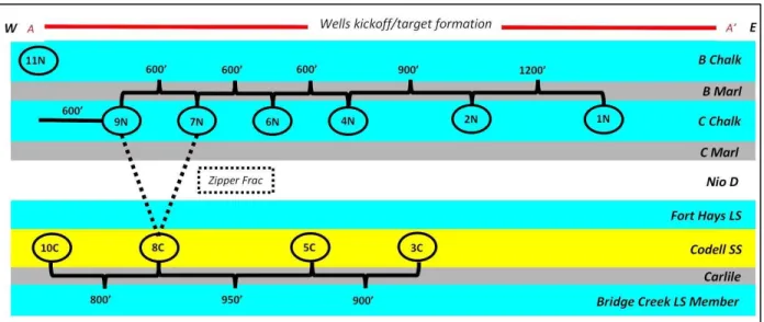
The Niobrara unconventional reservoir is a successful shale resource play due to the advances in horizontal drilling and hydraulic fracturing (Sonnenberg, 2013a). The Niobrara Formation is a self-sourcing interval of chalks and marls. The formation extends into several basins within the central US from Colorado, Wyoming, Nebraska and Kansas (Figure 1.1) (Sonnenberg, 2011a). The predominant exploration and development targets are located within the Denver Basin consisting of oil, condensate and gas accumulation. The purpose of this study is to assess the Niobrara reservoir stimulation treatment within one square mile section of Wattenberg Field (Figure 1.2). The analysis will be focused over the Reservoir Characterization Project (RCP) consortium data sets within a section that is targeting the Niobrara and Codell with 11 Horizontal wells.

The Niobrara Formation is an organic-rich, self-sourcing unit, predominantly made of carbonate deposits in the form of alternating layers of chalks and marls. The Niobrara resource play is typically compared to the Eagle Ford Shale due to its high carbonate content. Earlier production can be dated back to 1976 from vertical wells in Wattenberg Field, although not deemed commercially viable at the time. The shale play has become more attractive with the move towards horizontal drilling and multistage hydraulic fracturing allowing for the Niobrara to successfully be developed with overall success in the Denver basin ever since 2009(Sonnenberg, 2013a).

(21)

has a resource estimate of 3-4 billion barrels equivalent (Sonnenberg, 2013). The generalized stratigraphic column shown in Figure 1.1 shows the predominant members within the Niobrara Formation (alternating layers of chalk, in blue, and marl, in grey). The Niobrara Formation (Smoky Hill Member) consists of four limestone (chalk) units and three intervening marl intervals ranging in depth from 6200 - 7800ft MD (Sonnenberg, 2013). Within the study Reservoir Characterization Project study area (Figure 1.2), the Niobrara A chalk is not present. The main Niobrara reservoir intervals within the focused RCP study area are the Niobrara B chalk and Niobrara C chalk. The Niobrara Formation is bounded by the Sharon Springs member of the Pierre Shale above, and the Codell below. The Codell sandstone is also considered to be a tight reservoir that is usually targeted by horizontal drilling and hydraulic fracturing along with the Niobrara for its hydrocarbon bearing potential.

(22)

Figure 1.2 Location of the RCP study area within Wattenberg Field (RCP, 2017)

1.2 Project objective

The Niobrara Shale play is calculated to have a total of technically recoverable reserve around 3.7 billion barrels of oil and 46.5 Tcf of gas (IHS, 2016). These estimates are based on a 2-8% recovery rate per well. Advances in geological and geomechanical reservoir characterization, integrated with simulation modeling, has allowed the industry to improve recovery by modeling and analyzing the effectiveness of the hydraulic fracture stimulation to increase recovery factors from shale reservoirs (Wallace et al., 2016).

This project proposes the use of 3D hydraulic fracture simulation models for the characterization of hydraulic fracturing treatments in unconventional shale reservoirs. This project will focus on analyzing the changes in stress and pressure within the reservoir as a result of the hydraulic fracturing and production. The goal is to analyze the variations of in-situ stress and pore

(23)

seismic interpretation to assess the dynamic stress state of the reservoir for potential infill drilling and refracturing opportunities.

The motive behind this project is to characterize the hydraulic fracturing within the Niobrara to provide better insight into improving well spacing and hydraulic fracturing efficiency within Wattenberg Field. The project focuses on analyzing the changes in elastic rock properties, pressure and stress within the reservoir and their influencing effect on hydraulic fracturing using a 3D numerical reservoir simulator. The simulation results are integrated with microseismic observations in the area, along with the 4D seismic interpretations, to analyze and determine the effect of geological heterogeneity on hydraulic fracturing. The objective of this work is to understand how the in-situ stress variations within the reservoir affected the initial stimulation treatments. The insight provided by this study will help assess areas within the reservoir that are potential for infill drilling or re-fracturing.

The use of the 3D numerical hydraulic fracture simulator coupled with 4D/9C time-lapse seismic interpretation shows that there is still room for improvement to be made in optimizing well spacing and hydraulic fracturing efficiency within the Niobrara Formation. By understanding the reservoir complexity in regard to stress anisotropy, strength variation and natural fracture density, exploitation and optimization plans can proceed with better efficiency for potential increase in recovery from the Niobrara unconventional reservoir.

1.3 Project workflow

This integrated project will be conducted using different methods to obtain a sensible understanding of the hydraulic fracturing efficiency within the Wishbone section of the Wattenberg

(24)

1) Generate a 1D geomechanical mechanical earth model to assess the vertical stress distribution within the Niobrara and Codell Formations.

2) Generate a 3D geomechanical model to represent the lateral geologic and geomechanical heterogeneity within the Niobrara and Codell Formations.

3) Input the 3D geomechanical model into a 3D numerical reservoir simulator for hydraulic fracture characterization.

4) Integrate results from simulation modeling results with microseismic observations, along with 4D/9C time-lapse analysis to assess hydraulic fracturing efficiency.

5) Assess area for potential infill drilling and refracturing opportunities based from integrated the simulation results with the 4D seismic interpretations.

1.4 Data availability

The 3D seismic surveys and well log data within this study area was provided through the Reservoir Characterization Project (RCP) along with Anadarko Petroleum Corporation (Figure 1.3). The well logs provided for this project include the GR, RHOB, NPHI, Resistivity logs, along with some DT logs. Synthetic DTP and DTS logs were generated around the Wishbone section from Neural Network analysis based on empirical relationships established from offset wells that included real sonic data (Bray & Link, 2015; Pitcher, 2015). Core data taken from the Niobrara interval was also provided by Anadarko for several wells around the study area (Figure 1.3). All drilling and completion data, along with the production information (Figure 1.5), within the Wishbone section are also provided by Anadarko.

The 9C multicomponent 4D time-lapse seismic data (Baseline, Monitor 1, Monitor 2) was acquired by the RCP consortium over the Turkey Shoot area to obtain full fold over the Wishbone section, with a bin size of 50ft x 50ft (Figure 1.3) (RCP, 2016). The time-lapse nature of the seismic

(25)

first 9C seismic survey (Baseline) was acquired after drilling the 11 horizontal wells in the section (Figure 1.6 & Figure 1.7). Surface microseismic was captured while hydraulic fracturing of the 11 horizontal wells was being conducted (Figure 1.8). The following 9C seismic survey “Monitor 1” was acquired right after hydraulic fracturing was completed in the area to assess the seismic response caused by hydraulic fracturing and estimate a stimulated reservoir volume (SRV). Following 2 years of production, “Monitor 2” seismic survey was acquired to analyze the productive reservoir volume and assess the area for potential bypassed reserves.

The acquisition and processing of the time-lapse surveys focused on preserving the repeatability and consistency in regard to acquisition and processing to reduce the effect of noise caused by any inconsistencies in acquisition or processing. The time-lapse Baseline and Monitor surveys were processed simultaneously by Sensor Geophysical for the PP, PS and SS seismic data (RCP, 2016). Cross equalization of surveys was also applied on the overburden sections within the surveys to remove any noise resulting from any dissimilarities in acquisition. The cross equalization is an essential process for obtaining reliable differences at the reservoir level.

(26)

Figure 1.4 4D Time-lapse seismic timeline modified from (White, 2015)

Figure 1.5 Normalized Niobrara Production (left), Normalized Codell Production (right) showing over 50% variability in production performance between Niobrara Wells, and over

(27)

Figure 1.6 Cross section through the lateral wells relative to the target intervals. Cross section depicted in Figure 1.7 (RCP, 2017)

Figure 1.7 Variation in well landing intervals due to geologic heterogeneity and faulting. Modified from (Pitcher, 2015)

(28)

Figure 1.8 Acquisition geometry for surface microseismic FracStar array. The survey has 14 arms and 3396 channels (RCP, 2016)

1.5 Previous work

Several projects have been conducted within Wattenberg Field by the Reservoir Characterization Project (RCP) within Colorado School of Mines. The information provided by many of these projects helped develop a better understanding of the geological heterogeneity within the study area. The work provided by Matthies (2015) helped provide a regional understanding of the Niobrara depositional system. Brugioni (2017) described the core to observe the facies distribution within the Niobrara closer to the RCP study area. Their work was helpful in creating a fundamental understanding of geological heterogeneity within the Niobrara Formation.

Insight into characterizing the geomechanical complexity within the Niobrara over the RCP study area was previously provided by several RCP students. The FMI analysis was conducted

(29)

wells by Dudley (2015). While Mabrey (2016) provided insight into the lateral variability in geological heterogeneity along the horizontal wellbores targeting the Niobrara and their impact on the near wellbore stresses and geomechanical properties. A 3D seismic driven geomechanical model was also generated by Grazulis (2016) that helped provide valuable insight into the lateral distribution on stress with in the Niobrara Formation in the same given study area. Grazulis (2016) provided a glimpse into the effect of hydraulic fracturing and production on the reorientation of stress around select wellbores in the area. The insight provided by these students will help me develop a better understanding of the lateral distribution of in-situ stress within the Niobrara reservoir.

A 3D structural model including several faults and was generated by Ning (2017) to be used for production history matching. The structural model consisted of several seismic derived horizons that were depth converted using a 3D velocity model generated Payson Todd. The structural model generated by Ning (2017) will be used for my project to generate a 3D geostatistical model as well as a 3D hydraulic fracture simulation result that can be used as an input into Ning (2017)’s production history matching in the near future.

Dang (2016) assessed and analyzed the production tracers within the study area. She also provided some early insight into the geometry generated by hydraulic fracturing the Niobrara using a simple 1D geomechanical model. Her analysis will be taken into consideration to help further my understanding of the hydraulic communication between the wells and their potential impact on production from the Niobrara and Codell Formations.

(30)

The 4D-seismic multicomponent effects caused by hydraulic fracturing were also assessed by Mueller (2016) for mapping the stimulated reservoir volume through the application of time-lapse seismic shear wave inversion within the same study area. By integrated their work into the results provided by the 3D numerical reservoir simulator for hydraulic fracturing, I am able to develop a better understanding of the hydraulic fracturing efficiency in the area. The integration will also be important for assessing areas for potential enhanced recovery through infill drilling and refracturing.

This insight provided by many of the projects that were previously conducted over the same study area will constructively help guide the interpretation and analysis of my results. The goal of this project is to make use of previous work by integrating the information into a simulation model for hydraulic fracture characterization within the Niobrara. The potential recommendations that will be provided by this project will allow for better field development, increased hydrocarbon recovery, and increased overall production from the Niobrara through infill drilling and refracturing.

(31)

CHAPTER 2 RESERVOIR CHARACTERIZATION OF THE NIOBRARA FORMATION WITHIN

WATTENBERG FIELD

2.1 Summary

The Niobrara Formation is an organic rich and mature source rock interval. With advances in horizontal drilling and hydraulic fracturing, the Niobrara has become a valuable resource for hydrocarbon production. The variability in success within the Niobrara is driven by the reservoir quality and location of relative “production sweet spots” within the basin. The ability to characterize the Niobrara reservoir and produce from these “production sweet spots” can have a significant effect on the production rates from such wells, along with the overall hydrocarbon recovery. Understanding the effect of the geological heterogeneity within the Niobrara, and the effect of such heterogeneity on potentially increasing reserves and recovery is critical to any shale exploration or development program targeting the Niobrara Formation.

2.2 Introduction

The Niobrara unconventional resource has become an attractive and successful shale reservoir targeted ever since 2009 due to the advances in horizontal drilling and hydraulic fracturing, while early production can be dated back to 1979 (Sonnenberg, 2013a). The Niobrara resource play extends in several basins within the central US from Colorado, Wyoming, Nebraska and Kansas. The predominant exploration and development targets are located within the Denver Basin consisting of oil, condensate and gas accumulation.

(32)

billion barrels of oil and 46.5 Tcf of gas, or 11.5 billion barrel of oil equivalent as shown in Figure 2.1 (IHS, 2016; U.S. Energy Information Administration, 2011). Comparing this estimated volume to database for the main shale resources, it can be observed that recoverable gas in the Niobrara is range in the middle of the group. For recoverable oil, the Niobrara is comparable to the Bakken and Eagle Ford.

The Niobrara Formation acts as its own reservoir and source interval (Figure 2.2). The self-sourcing nature of this reservoir target, along with the low permeability of the formation, makes for an attractive unconventional hybrid system to be targeted for hydrocarbon extraction using horizontal wells and hydraulic fracture treatments. The Niobrara Formation (Smoky Hill Member) consists of four limestone (chalk) units and three intervening marl intervals ranging in depth from 6200 - 7800ft MD within the Denver-Julesburg (DJ) Basin, Colorado, with thicknesses ranging from 150ft - 1500ft. The Niobrara Formation is a self-sourcing unit that has TOC values ranging from 1-5%. The organic matter is of type II kerogen (oil prone) (Sonnenberg, 2013a).

(33)

2.3 The Niobrara petroleum system

The Niobrara Formation (Late Cretaceous age) was deposited in a foreland basin setting in the Western Interior Cretaceous Seaway of North America during a time of a major marine transgression (Sonnenberg, 2013a). The present-day basins in which the Niobrara deposits currently reside formed during the Late Cretaceous to Early Tertiary Laramide orogeny within the Rocky Mountain Regions. The sediment deposits that formed the Niobrara Formation (Smoky Hill Member) consist of four limestone (chalk) units and three intervening marl units (Figure 1.1). The alternating layers of chalk and marl make the Niobrara Formation a prime target for unconventional resource exploitation due the self-sourcing nature of the reservoir and low permeability that allows for the hydrocarbons to be trapped soon after generation (Figure 2.2).

Figure 2.2 Niobrara Petroleum System Event Chart (Finn & Johnson, 2005)

The Niobrara Formation is predominantly located within areas northeast Colorado, and parts of Wyoming, Nebraska, and Kansas (Figure 1.1). The Niobrara Formation is actively drilled and being developed in the Denver-Julesburg Basin, Colorado, using horizontal drilling and hydraulic

(34)

and marls. The Niobrara resource play is typically compared to the Eagle Ford Shale due to its high carbonate content.

The generalized stratigraphic column in Figure 1.1 shows the alternating layers of chalk, in blue, and marl, in grey, within the Niobrara. The Niobrara Formation is made up of two members, the Smoky Hill Member and the Fort Hays member. The Smoky Hill member is a target for unconventional resource exploitation. The Smoky Hill member consists of limestone (chalk) units and intervening marl intervals ranging in depth from 6,200 – 7,800ft MD within the DJ Basin, Colorado. The Niobrara Formation is bounded by the Sharon Springs-Pierre Shale above (top seal), and the Codell Sandstone below (Sonnenberg, 2013a).

The Wattenberg Field within the Denver Basin is the most active area producing from the Niobrara Formation. The Wattenberg area covers approximately 3200 square miles, and has a resource estimate from the Niobrara of 3-4 billion barrels equivalent (Sonnenberg, 2013a). The formation averages a thickness of 3,500ft. Composed of Cretaceous carbonate deposits, the Niobrara can range in thickness from 150ft to 1,500ft thick with a general thinning direction towards the east of the Rocky Mountain Region. Organic content within the Niobrara is of Type II (oil prone) kerogen (Figure 2.3), with TOC values in the range from 1% to 5% (Sonnenberg & Weimer, 1993).

Based on thermal maturity mapping, the Niobrara shale has predominantly entered the proper maturation windows for generating oil and gas. The Niobrara Formation is immature to the east of the Denver Basin and more mature to the west with production varying accordingly. Vitrinite reflectance values range from 0.6-1.3 Ro within the Denver basin (Figure 2.4). Both thermogenic and biogenic petroleum accumulations can occur within the Niobrara. The accumulations in the deep part of the basin are thermogenic oil and gas; whereas, the

(35)

The Niobrara is observed to be abnormally pressured within the Denver Basin with pore pressure gradients ranging between 0.41-0.67 psi/ft (Figure 2.5) (Sonnenberg, 2011a; Luneau, Longman, Kaufman, & Landon, 2011).

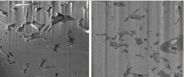
Petrophysical evaluation of the well logs shows that the chalks possess higher porosity values that average between 11-13% than the marls that have average porosities less than 11%. FESEM analysis confirmed the presence of organic pores, interparticle and intraparticle pores that vary in morphology (ranging in size from 3 microns to less than a micron) within the Niobrara Formation (Elghonimy, 2015). These micro pores range from 1.4%-10% porosity (Figure 2.6) (Michaels & Budd, 2014). These nanoscale pores capture and entrap the hydrocarbons within the formation right after the generation of hydrocarbons occurs. The hydrocarbons have a difficulty to escape from these nanoscale pores due to the very low permeability within the shale reservoir that predominantly range below 0.1mD (Sonnenberg, 2012).

(36)

Figure 2.4 Thermal maturity map of the active source rocks within the DJ basin modified from (Higley & Cox, 2007)

(37)

Figure 2.5 Overpressure trend within the Niobrara (Sonnenberg, 2011a) modified from (Weimer, Sonnenberg, & Young, 1986)

Figure 2.6 SEM images interparticle porosity (left) and kerogen porosity (right) from the Niobrara Formation. Left image is 12.7 microns across, right image is 8.5 microns across

(38)

2.4 Faults and fractures within the Niobrara

Various stages of tectonic activity had an influence on the faulting and fracturing of the Niobrara Formation within the Denver Basin as a result of the Laramide Orogeny and the Neogene extension (Figure 2.2). The region has undergone uplift, strike slip wrench faulting, and normal faulting as result of the tectonic activity in the area (Figure 2.7). Faults and fractures that resulted from the tectonic events within the region caused several fault patterns to occur in different directions. These faults and fractures can significantly enhance the permeability of the formations and favorably impact production within many parts of the basin. The Niobrara Formation is observed to exhibiting polygonal faulting in some areas within the basin as result of the compaction and dewatering of the shale units (Sonnenberg & Underwood, 2013). These fault patterns observed in seismic sections within the Niobrara are of small extent (10-50m, 30-70° dip), layer bounded, and randomly oriented (Sonnenberg & Underwood, 2013).

The natural fractures within the Niobrara Formation are very important for their significant effect on production and hydraulic fracture propagation within shale reservoirs. Natural fractures enhance the flow permeability within the Niobrara Formation. The matrix permeability is very low in shales. Having an abundance of natural fractures pre-existing within the rock fabric is very good for enhancing the flow of hydrocarbons from the shale formation to the wellbore. The abundance of natural fractures within the Niobrara can significantly affect the hydraulic fracturing within the formation. The natural fractures can help with maximizing the reach of the hydraulic fracture treatment and help enhance the conductivity within the reservoir. Natural fractures can enhance flow conductivity and permeability to allow for more hydrocarbons to be produced from the reservoir through the natural fractures.

(39)

(40)

2.5 Geomechanical considerations for hydraulic fracturing

The Niobrara Formation consists of an abundance of calcite (chalk), quartz, feldspar, and clay minerals (marls). Figure 2.8 shows an example of the variation in mineral distribution within the Niobrara through a vertical section crossing through the Niobrara A, B, C and Fort Hays. The amount of clay is variable throughout the vertical section ranging from 5-20%, averaging at 10% for the entire interval. Clay content is shown to decrease in the chalk intervals, and increase in the marl intervals. Having low clay content within the Niobrara Formation makes it more favorable for hydraulic fracturing.

The variability in clay (ductile minerals) versus brittle minerals has a significant effect on the strength of the formation and the ability to hydraulically fracture it. The effect of both the stress magnitude and the strength of the formation both play an important role in allowing for an effective hydraulic fracture treatment to take place. Strength anisotropy within the Niobrara is directly affected by the lateral heterogeneities within the shales mineralogical composition and stress condition. The amount of clay, silica, carbonate and organic content within the shale reservoir significantly affect the hardness or brittle nature of rock (low clay content), or soft ductile behavior (high clay content) that the reservoir can have as a result of hydraulic fracture treatments.

The diagram in Figure 2.9 from Sonnenberg’s lecture series on the Niobrara Formation illustrates the distribution of calcite, feldspar and clay minerals within the Niobrara Formation relative to other successful shale plays within the US. The diagram also separates between the clay rich shales and the brittle shales thus illustrating that the Niobrara is believed to react in a brittle manner to hydraulic fracturing similar to the Eagle Ford due to its high calcite content and low clay content.

(41)

Figure 2.8 XRD analysis of the Niobrara core sample within the DJ Basin (Elghonimy, 2015; Sonnenberg, 2012)

(42)

The mineralogical strength related properties within the Niobrara Formation are stress dependent. In-situ stress conditions affecting the shale reservoir play a significant role in the ability to hydraulically fracture the formation. Understanding the regional and local stress variations affecting the reservoir, exploitation and optimization operations can make use of the regional and local stress variations to propagate larger fracture treatments within the reservoir and allow for a larger stimulated reservoir volume to be induced onto the reservoir.

Using the stress affecting the reservoir, the reservoir can be exploited by drilling a lateral well (horizontal well) in the direction of minimum horizontal stress, and hydraulically fracturing the reservoir in the direction of maximum stress. The induced fracture network will dilate in the direction of minimum horizontal stress, and be more likely to stay open after hydraulic fracturing. The stress regime affecting the reservoir helps with initiating and maximizing the extent of the hydraulic fracture in the direction with least resistance (in the direction of maximum horizontal stress). The transverse induced fracture network helps with enhancing conductivity and permeability between the wellbore and the formation. This encourages flow within the reservoir to the wellbore, and increases the size of the stimulated reservoir volumes that favorably impact EUR and production rates.

Current day stress regimes are thought to have significant effect on the fracturing and the conductivity of the open fractures within the areas. As observed in Figure 2.10, the maximum horizontal stress direction within the regional extent of the Denver Basin is approximately in the WNW-ESE direction. Local stress variations can occur and change in azimuth from section to section throughout the Denver Basin. Understanding the current day stress regime is very important for the drilling and hydraulic fracturing operations to be conducted to be taken advantage of when hydraulically fracturing the Niobrara Formation.

(43)

Figure 2.10 Principal horizontal stress distribution and orientation within the US (Zoback & Zoback, 1980)

The local variations in stress directions play a significant role in controlling the ability for a fault to act as a barrier, or a conduit, to flow within the reservoir. Given that induced hydraulic fractures tend to dilate in the direction of minimum stress, any faults or fractures oriented parallel to the direction of maximum stress are more likely to act as conduit to flow and enhance the stress dependent permeability within the Niobrara Formation. Faults and fractures oriented perpendicular to the maximum stress direction are more likely to be sealing faults. Assessing the local variations in stress orientation is very important to drilling and hydraulic fracturing, as well as making use of these complex fracture networks within the Niobrara Formation for generating larger SRV and PRV areas around the horizontal shale wells.

(44)

2.6 Production “sweet spots” based on reservoir quality

Prospectivity within the Niobrara unconventional play, similar to any other unconventional resource, is highly dependent on the geological heterogeneity. The ability to understand the reservoir heterogeneity and make use of the geological and geomechanical information to best assess the area for production sweet spots can favorably affect production rates. In order to detect these production sweet spots within Niobrara Formation, the reservoir must be assessed for properties pertaining to organic richness, maturity, mineralogy, brittleness, thickness, pore pressure, porosity, permeability, natural fractures (Figure 2.11).

The key reservoir properties of the Niobrara reservoir and other main unconventional shale plays are compared in Table 2.1. Similar to every other successful unconventional shale gas/oil in the US, the Niobrara Formation has all the required properties to be technically and commercially produced. Identifying the local sweet spots within the Denver Basin can favorably increase and enhance production, and EUR from the Niobrara reservoir.

(45)

Table 2.1 Comparison between Niobrara Formation to other unconventional shale based on EIA, 2011 assessment (U.S. Energy Information Administration, 2011)

Barnett Bakken Marcellus Niobrara

Depth 6500-8500ft 1000-9000ft 4000-8000ft 6800-7100ft

Net thickness 100-600ft 20ft 50-250ft 120ft

TOC 4.5% 5-20% 1-5% 1-6%

Clay content <35% <20% 20-35% 10%

Porosity Average ~4.5% 5.5-9% 1.6-7% 2-8%

Lithology Siliceous shale, Calcareous layer

Shale, Dolomite, Siltstone

Shale, Limestone Chalk, Marl

2.7 Drilling & completion strategy within Wattenberg Field

Within the Denver Basin, horizontal wells are most common and will soon replace all the vertical well as it proves to be more effective for producing from tight oil reservoirs similar to the Niobrara (Hughes-Fraire & Olmstead, 2015). The Niobrara Formation has a similar completion procedure and technique to any other unconventional play. The typical drilling and spacing unit for the new horizontal wells is generally 640 acres. The wells are generally oriented perpendicular to the maximum horizontal stress direction within the area to optimize the fracture stimulation and align the induced fractures with the current principal stress direction. The Niobrara Formation is a comprise of chalk and marl. Hydraulic fracturing will focus on the chalk layer which result in a better stimulated fracture network. Figure 2.12 shows the comparison of drilling parameters and cost between the Niobrara and Bakken.

(46)

Figure 2.12 Comparison of drilling parameters and cost between the Niobrara and Bakken (Sonnenberg, 2012)

Within the RCP study area, horizontal wells targeting the Niobrara and Codell reservoirs are drilled in a single layer interval, such as the Niobrara B, C, and Codell. An array of horizontal wells typically alternates between two formations such as the Niobrara C and Codell. The fracturing is then performed in the first well and then the second well which is drilled on the adjacent formation, and then the third well which is drilled in the same formation as the first well. By alternatively fracturing between two formations, operators can use the occurrence of stress shadow in order to stimulate a larger reservoir volume and induce a more complex fracture network. In addition, fracturing stage sequence such as zipper fracturing can also be performed to enhance SRV. Fracture staging can be as high as 30+ stages per horizontal well.

“Sliding sleeve” and “plug and perf” fracturing methods commonly used in the Niobrara (Paterniti & Losacano, 2013). Choosing which technique to use is dependent on a company’s preference such as time, cost and trial and error experience. Sliding sleeve involves less operation cost, time and effort as all the fracturing process can be done within a single string of sleeves and no casing and perforation are required. On the other hand, even though the plug and perf requires more effort the benefit of doing plug and perf is that you will be able to customize

(47)

your perf zone and can always go back and re-perf the zone of interest (Fry, Roach, Kreyche, Yenne, & Geoffrey, 2016).

Persons (2015) discussed fracturing techniques in the Niobrara and mentioned that there is no conclusion on which method is better in the Niobrara as horizontal drilling is now in the early stage and there is not enough statistical information (Persons, 2015). Hybrid fracturing operations using the two techniques can also be performed but it will require a relatively higher operating cost. However, RCP’s study would indicate that plug and perf is the better option at this time.

2.8 Conclusions

The Niobrara Formation is a self-sourcing reservoir that consists of inter-bedded layers of chalk (reservoir rock) and marl (source rock). The Niobrara Formation has a relatively low clay content and is considered to be an attractive target for oil and gas production. Economic production from the Niobrara reservoir requires the use of horizontal drilling along with hydraulic fracturing. The depth ranges around 6,200 - 7,800ft MD with the net thickness of at least 120ft which are in the range and thickness that horizontal drilling and fracturing can be effectively performed.

The Niobrara has gone through a number of active tectonic phases throughout geological history, and is likely to be highly fractured and faulted in many areas within the basin. The effect of these faults is still uncertain, but the common belief is that these faults can act as baffles and conduits to flow depending on a number of geological and stress dependent factors. The Niobrara reservoir formation is brittle, naturally fractured, thermally mature to generate oil, condensate & gas. Overall, just like every other producing unconventional shale resource in the U.S., the

(48)

Table 2.2 Shale reservoir properties as compared to other successful shale plays within the U.S. (Luneau et al., 2011)

The Niobrara resource play is calculated to have a total of technically recoverable reserves of 3.7 billion barrels of oil and 46.5 Tcf of gas (IHS, 2016). These estimates are based on typical reserve recovery factors within these unconventional reservoirs can range as low as 2-8%. There is still much improvement to be done in order to increase the recovery from the Niobrara reservoir. Through geological and geomechanical characterization, reservoir and production sweet spots can be identified within the Niobrara Formation to allow for better hydrocarbon recovery and production to occur.

(49)

CHAPTER 3 ASSESSING THE NIOBRARA SHALE RESERVOIR FOR HYDRAULIC FRACTURE

COMPLETION QUALITY USING WELL LOGS

3.1 Summary

The Niobrara requires the use of hydraulic fracturing to be productive. Multistage hydraulic fracturing is needed to yield economic production from the Niobrara Formation. Evaluating the intervals within the Niobrara Formation for favorable hydraulic fracturing is essential for generating an efficient connection between the hydrocarbon bearing formation and the producing wellbore through hydraulic fracture stimulation. Determining the geomechanical properties within in-situ conditions along with the reservoir pressures is the first step to evaluating unconventional shales for hydraulic fracturing. This chapter discusses methods used to characterize and predict the reservoir elastic rock properties, pore pressure, and magnitude of stress affecting the Niobrara and Codell Formations using well log data to assess which intervals within the reservoirs should be targeted for better containment and more favorable stimulation treatments to take place.

3.2 Introduction

Shale reservoirs require hydraulic fracturing to be successful and productive at economical rates. Identifying the ideal target intervals for hydraulic fracturing is an essential first step before drilling generally takes place. Targeting and stimulating the more favorable layers within a reservoir for hydraulic fracturing can significantly increase the production performance out of a treatment well. Shale reservoir intervals that are more favorable for hydraulic fracturing typically

(50)

better understanding of the vertical level of heterogeneity that will have an effect on the optimum well placement for better containment and more effective fracturing to take place.

Stress modeling and prediction within shale reservoirs is a critical and important step required to understand the hydraulic fracture containment within the target intervals. As previously discussed in Chapter 2, the Niobrara Formation is abnormally pressured (Figure 2.5). The pore pressure trend surrounding the Niobrara Formation will have an influencing role on the vertical and lateral stress distribution within the target formation. Quantifying and predicting the reservoir elastic rock properties, pressures and stress profiles within the Niobrara Formation is essential for characterizing the Niobrara Shale Reservoir for hydraulic fracturing. Estimating the elastic rock properties, pressures and stress distribution above and below the Niobrara Reservoir is equally as important to assess the fracture containment within the reservoir, and predict which intervals within the Niobrara are more optimum for hydraulic fracturing.

3.3 Data available for well log analysis

The vertical wells surrounding the Wishbone study area are used for assessing the Niobrara from a geomechanical perspective. The wells shown in Figure 3.1 are selected for containing the logs necessary for this analysis to be conducted. The logs available are Gamma Ray (GR), Density (RHOB), Neutron Porosity (NPHI), Deep Resistivity (ILD). Sonic logs (DTP & DTS) were estimated from Neural Network correlation (Bray & Link, 2015; Pitcher, 2015). Figure 3.1 shows the location of these wells relative to the study area. The 11 lateral wells within the section only consist of Resistivity and GR logs that were used to geosteer the wells into their landing intervals.

(51)

Figure 3.1 Top Niobrara depth map over model area. The wells (colored in black) represent the 13-vertical used for predicting the geomechanical properties

3.4 Estimating elastic moduli from well logs

The fundamental purpose of this step in the project is to derive the geomechanical properties that will go into the calculation of the minimum horizontal stress equations. The log derived geomechanical parameters within the Niobrara are stress and time dependent. The properties that are calculated within this chapter represent the static reservoir conditions at the time of drilling. Considering that the area is actively drilled and hydraulically stimulated, the properties might be altered at a later stage and will have a considerable effect on any infill drilling or hydraulic fracturing that proceeds this study. The geomechanical properties estimated using the well log data represent the static geomechanical properties in-situ before hydraulic fracturing or production. These measurements will represent the initial state condition of the reservoir units

(52)

The most important parameters for the derivation of the minimum horizontal stress magnitude are the Young’s Modulus (the ratio of extensional stress to extensional strain in a uniaxial stress state), and the Poisson’s Ratio (the negative ratio of the radial strain to the axial strain in a uniaxial stress state) Equations (3.1) & (3.2) (Mavko, Makerji, & Dvorkin, 2009). Both these properties are stress dependent parameters. The change in overburden stress and formation pore pressure (effective stress) directly influences the measurements of Poisson’s and Young’s moduli in-situ conditions.

Young’s Modulus E

=

σ_�ax�al

ax�al (Eq. 3.1)

Poisson Ratio

 =

−

�

_�

ax�al

ax�al (Eq. 3.2)

The measurement of these elastic properties is typically derived from laboratory experiments applied onto core samples of rock to obtain static and dynamic measurements. In areas with little to no core samples, the dynamic elastic properties can be calculated using P-wave and S-wave velocities (Mavko et al., 2009) using equations (3.3) & (3.4). The dynamic log properties can then be calibrated to core samples when made available to infer a static type measurement. Generally, core (static) measurements are observed to be lower than the log (dynamic) obtained estimates for Young’s modulus and Poisson ratio (static measurements < dynamic obtained estimates). Using the static converted measurements is very important, the use of dynamic properties might be very misleading.

=

�⁄ � −

�⁄ � − (Eq. 3.3)

(53)

Although these elastic moduli can easily be obtained from dynamic logs, they require proper matching to core data (static measurements) to be used to calculate the minimum horizontal stress magnitude pressures. The correlations developed by Eissa and Kazi (1988) are generally considered to be a reliable method for obtaining a static conversion from dynamic log calculated data. The dynamic to static correlation has been modified by van Heeran (1987) along with Barree (2009) to produce a more reliable correlation between static and dynamic moduli measurements in the laboratory modified from (Eissa & Kazi, 1988).

The plot depicted in Figure 3.2 shows a comparison between these widely used techniques at predicting the static measurements from dynamic velocity data through core experiments data (Barree, Gilbert, & Conway, 2009). Converting the Poisson’s Ratio measurements from dynamic to static log data on the other hand appears to be less important as apparent in Figure 3.3 (Barree, Gilbert, et al., 2009). The relationship between PRdynamic and PRstatic is very close to 1:1.

= . − . linear correlation (Eissa & Kazi, 1988) (Eq. 3.5) = � − . log-linear correlation (Barree et al., 2009) (Eq. 3.6) = . . 79 _{power law model} _{(van Heerden, 1987) (Eq. 3.7)}

The calculated values for Poisson’s ratio and Young’s modulus from the conversion from dynamic to static are depicted in Figure 3.4. The static converted values using the log-linear correlation are in accordance with observations made from core analysis by (Bridges, 2015; Maldonado, 2011). These static converted measurements will be used as input parameters to the calculation of the minimum horizontal stress equations in the following sections within this chapter.

(54)

Figure 3.2 Correlations between dynamic to static Young’s modulus from core data (Barree, Gilbert, et al., 2009)

Figure 3.3 Correlation between dynamic to static Poisson’s ratio measurements from observed core data (Barree, Gilbert, et al., 2009)

(55)

A brittleness factor (BRF) is also computed using correlations based on Young’s modulus and Poisson’s ratio (Rickman, Mullen, Petre, Grieser, & Kundert, 2008). The brittleness factor is used as a reference to the fracability of the formation, it does not go into the stress calculations. It helps to identify intervals within the Niobrara that are more favorable for hydraulic fracturing. According to Rickman et. al. (2008), shale intervals with low Poisson ratio’s and higher Young’s Modulus are more favorable for hydraulic fracturing and will tend to react in a more brittle manner (Figure 3.5).

= . × � – . × PR � + . (Rickman et al., 2008) (Eq. 3.8)