Interaction Delay and Marginal Cost in Swedish Bicycle
Traffic
Fredrik Johansson (VTI) Roger Pyddoke (VTI) CTS Working Paper 2018:19 Abstract
We apply the method presented by Johansson (2018) to estimate a volume delay function and marginal cost for bicycle traffic on cycling paths separated from motorized traffic based on point measurements of speed and lateral positions from seven sites in Sweden. The results indicate that a quadratic volume – delay function fits the data well in the observed range of volumes, and that there are significant delays already at volumes far below the capacity due to the heterogeneity of the desired speed over the population. The total marginal cost of delay per unit flow is estimated to €9×10⁻⁵ h/km.
Keywords: Bicycle traffic, Delay, Marginal cost JEL Codes: R40; R41
Centre for Transport Studies SE-100 44 Stockholm
Interaction Delay and Marginal Cost in Swedish
Bicycle Traffic
Working paper
Fredrik Johansson*and Roger Pyddoke
VTI, Swedish National Road and Transport Research Institute, Box 8072, 402 78 Gothenburg
October 12, 2018
Abstract
We apply the method presented by Johansson (2018) to estimate a volume de-lay function and marginal cost for bicycle traffic on cycling paths separated from motorized traffic based on point measurements of speed and lateral positions from seven sites in Sweden. The results indicate that a quadratic volume – delay function fits the data well in the observed range of volumes, and that there is significant delay already at volumes far below the capacity due to the heterogeneity of the desired speed over the population. The total marginal cost of delay per unit flow is estimated to €9· 10−5h/km.
1 Introduction
The interaction delay and its socioeconomic cost has since long been investigated in detail for motorized traffic. Corresponding investigations of bicycle traffic has, until recently, not been made due to the limited congestion in bicycle traffic. How-ever, Hoogendoorn and Daamen (2016) proposed a method to estimate desired speed distributions in bicycle traffic and based on this Johansson (2018) proposed a method to estimate a volume delay function and marginal cost.
Here we apply the method presented by Johansson (2018) to data from seven sites in Sweden to estimate an average volume – delay function and marginal cost for separate bicycle paths of average characteristics.
2 Data
The data analyzed in this paper was collected using the automatic Viscando OTUS3D system, which for each detected road user provides a time stamp, type (pedestrian or cyclist), direction, speed, and lateral position. Data was collected at seven cy-cling paths in Sweden, all with similar characteristics: bidirectional bicycle traffic separated from a pedestrian path with a road marking or low curb, except in the Valla case which is a shared pedestrian and cycling path. All paths are separated from motorized traffic with a physical barrier, curb, or grass. That is, all have a rather typical design for high volume cycle paths in Sweden.
The reason for choosing so similar sites is to enable investigation of the vari-ability of the estimated volume delay function for this common type of infrastruc-ture. Also, to enable investigation of a large range of volumes, sites with known or suspected high volumes were chosen. This was also the reason for choice of time of year for data collection; late spring and early fall was chosen to capture the largest commuter flows (Pyddoke, 2018). The data from Danviksbron was not collected as part of the research presented in this paper, but was available from an earlier project.
The sample sizes and approximate effective widths of the cycling paths are pre-sented in table 1. By effective width is meant the width used by the overwhelming majority of cyclists, see fig. 4 to fig. 10 in appendix A for the detailed distributions of various road users across the road at the measurement cross section. As evi-dent from table 1 the widths of the cycling paths are similar, 2 m–2.5 m, except for Delsjövägen which is significantly wider with its 3.5 m and Valla, where cyclists share the 3 m width with pedestrians.
Table 1: Summary of data collection site properties
Site City # Cyclists Width Max flow Month
[m] [h−1]
Danviksbron Stockholm 2891 2 700 Aug
Valla Linköping 28485 3 500 May
Ullevigatan Gothenburg 22892 2.5 600 Sep
Delsjövägen Gothenburg 14905 3.5 500 Sep
Liljeholmsbron Stockholm 21577 2 1100 Sep
Munkbroleden Stockholm 41551 2.5 1700 Sep
Strandvägen Stockholm 22882 2.5 800 Sep
Total 155183
Except in the Valla case, the bicycle flows are rather well separated from both opposing bicycle flow and the pedestrian flows, implying that the main source of interaction delay at the sites are cyclists traveling in the same direction. Most of
the lateral distributions have tails outside of the main stream, which motivates the need to introduce a cut-off in lateral displacement from the mean lateral position to avoid artificially large headways and a thereby biased headway distribution, as described by Johansson (2018).
A short video from the Munkbroleden site was available for validating the data collection method. The video was recorded during the afternoon peak using a hand-held camera, and analyzed manually. The results indicate that the detector fails at detecting some cyclists in dense platoons, but no failures were observed for cyclists with a gap larger than a couple of meters to those in front and be-hind. These detection failures obviously lead to an underestimation of both the volumes and delays, but also to the delay at a given flow, since detection only fails for cyclists in platoons. Another effect of these detection failures is that the dis-tributions of following headways, estimated as part of the method to estimate the delays, get biased toward larger headways, which is consistent with differences between the distributions estimated in this study and those reported by Hoogen-doorn and Daamen (2016).
The flows exhibit typical morning and afternoon peaks at all the sites. At most of the sites the afternoon peak is significantly wider, and thus not reaching as high peak flows, and at Liljeholmsbron there is an alternative route that is preferable when cycling from the city center, further reducing the height of the afternoon peak, see fig. 11 to fig. 17 in appendix B. The flows at Munkbroleden are particu-larly large, peaking at around 1700 cyclists/h, which indicates that the capacity of also the other roads are much larger than the present maximum flows, due to the similarities between the infrastructure design at the various sites. Approximate peak flows, aggregated over 30 min intervals, are summarized in table 1.
The data was divided into separate sets for each direction and for the morn-ing and afternoon peaks, givmorn-ing a total of 26 data sets. However, only the sets with significant volumes were analyzed, as presented in table table 2. This di-vision of the data into subsets is motivated by that flow characteristics, such as desired speed and headway distributions, may vary between directions and time of day, so the method by Hoogendoorn and Daamen (2016) needs to be applied to each separately to estimate one desired speed distribution and one probability of following function for each direction and peak.
3 Results
For some of the data sets in table 2 the method proposed by Hoogendoorn and Daamen (2016) resulted in a poor estimate of the free headways, possibly due to too large deviations from exponential free headway distributions or too much interaction with pedestrians or opposing bicycle traffic. The data sets for which the headway model was successful are indicated in table 3.
Table 2: The division into data sets for each direction and peak.
Set nr Site Direction Peak
1 Danviksbron From Center Afternoon
2 Valla To Univ. Morning
3 From Univ. Afternoon
4 Ullevigatan To Center Morning
5 From Center Afternoon
6 To Center Afternoon
7 Delsjövägen To Center Morning
8 From Center Afternoon
9 Liljeholmsbron To Center Morning
10 To Center Afternoon
11 From Center Afternoon
12 Munkbroleden To Center Morning
13 From Center Afternoon
14 Strandvägen From Center Morning
15 To Center Afternoon
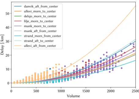
The volume – delay functions resulting from the method proposed by Johans-son (2018), are presented in fig. 1. Note, however, that the curves are extended beyond the flow levels present in the data for all data sets except for data set 12 to facilitate comparison. The scatter plots and fitted curves for each data set are presented in fig. 18 to fig. 26 in appendix C.
As can be seen in fig. 1, the estimated volume delay curves are relatively close to each other, with the exception of data set 5, which has a significantly steeper relation between volume and delay. This may be due to that there is a series of signalized intersections upstream of the measurement site, which bunch the traffic to dense platoons that may not have had time to disperse before arriving at the site.
To estimate an average volume – delay function, the data sets consisting of delays aggregated over one-minute intervals are combined into a single data set see table 3. The delays form data set 5 is excluded from the combined data set since the traffic conditions seem to differ significantly compared to the others.
The marginal costs are obtained by differentiation of the fitted quadratic delay functions multiplied by the value of time, as described in Johansson (2018). Given a total delay on the form δ = aq2, this gives a total marginal cost of c(q) =
2Caq, where C is the value of time, here taken as the standard recommended Swedish value, C = €12, from ASEK (2018). The values presented in table 3 are the marginal cost ’per cyclist’. That is, if we observe constant conditions for one unit of time and one km, then the values presented in table 3 are the additional
0 500 1000 1500 2000 2500 Volume 0 10 20 30 40 50 Delay [/km] danvik_aft_from_center ullevi_morn_to_center delsjo_morn_to_center lilje_morn_to_center munk_morn_to_center munk_aft_from_center strand_morn_from_center strand_aft_to_center ullevi_aft_from_center
Figure 1: Volume – delay functions of the form δ = aq2, estimated using the
various data sets.
costs of delay over the observed kilometer for each of the cyclists passing during the observed unit of time, caused by increasing the flow with one cyclist per unit of time.
The combined sets of delays for all data sets included in the combined data set are presented in fig. 2. As can be seen in the figure, The quadratic volume – delay function closely follows the mean of the data points up to around 2000 cyclists/h; above this level any estimate is uncertain due to the scarcity of data. The re-sulting combined estimate of the marginal cost is €0.9 h/km, obviously strongly influenced by the data from Munkbroleden, due to the large flows at this site. As is evident from the figure, most of the data sets agree well on the general shape of the volume – delay function, which is also reflected by the consistency of the estimates of the marginal costs in table 3.
The total and marginal delays presented above may be hard to relate to the individual experience of the cyclists. A more intuitive view of the amount of delay experienced by an individual cyclist is the delay experienced relative to the travel time at the desired speed. This is presented for the Munkbroleden data in fig. 3. As can be seen in the figure, there is significant relative delay already far below the capacity. The relation between the relative delay and the flow is close to linear with an increase of slightly below one percent relative delay per 100 cyclists/h flow.
Table 3: Estimated marginal costs for the data sets. Value in brackets denote an outlier not included in the combined data set.
Set nr Data set Marginal cost
per cyclist/h (2Ca) [€× 10−4h/km]
1 Danvik from center, afternoon 1.2
4 Ullevigatan to center, morning 0.82
5 Ullevigatan from center, afternoon [ 2.1 ]
7 Delsjövägen to center, morning 0.79
9 Liljeholmsbron to center, morning 1.0
12 Munkbroleden to center, morning 0.90
13 Munkbroleden from center, afternoon 0.78
14 Strandvägen from center, morning 0.62
15 Strandvägen to center, afternoon 1.2
Combined 0.9 0 500 1000 1500 2000 2500 Volume 0 5 10 15 20 25 30 Delay [/km]
aq
2 Delay Mean delayFigure 2: Total delay aggregated at the one-minute level combined from all data sets together with the mean for each flow level and errorbars representing ± 2 standard deviations of the mean. Also the estimated quadratic volume – delay function is included.
500 1000 1500 2000 2500 Volume 0.00 0.05 0.10 0.15 0.20 0.25 Relative delay
Figure 3: Delay relative to the preferred travel time, aggregated at the one-minute level for the data from Munkbroleden site during the morning peak in the direc-tion to the city center.
4 Conclusions
We conclude that the method presented in Johansson (2018) is able to estimate volume – delay functions and marginal costs for most of the data sets. The fail-ures at some of the data sets are likely due to deviations from the assumption of exponentially distributed large headways in these data sets.
Quadratic volume – delay functions fit the data well, and the estimated marginal costs at the sites with similar characteristics, (that is excluding data set 5), are within±34% of the combined estimate of €9 · 10−5h/km. Note, however, that the
quadratic form of the volume – delay function fit the data well in the observed flow range, there is no reason to believe that this is still the case for flows closer to capacity.
We also conclude that due to the large heterogeneity in desired speeds, cyclists start experiencing delay far below the capacity, which is an important difference to motorized traffic where the desired speed distribution is concentrated close to the speed limit, leading to relatively small delays in an extended free flow range.
5 Discussion
To exemplify the size of the marginal cost, consider the case of the peak morning flow at Munkbroleden: Each of the mornings Tuesday to Thursday have at least one 15 min interval with a flow of 1750 cyclists/h. If we increase the flow with one cyclist per hour, each cyclist will get an additional delay of a value accord-ing to table 3 per kilometer traveled. Assume that we have an kilometer stretch with homogeneous conditions around the measurement site. The value of the ad-ditional delay accumulated over this kilometer stretch by all the cyclists passing the site during the 15 min peak if the flow is increased by one cyclist per 15 min is c(1750) = €0.9· 10−4· 1750 ≈ €0.16. The peak flows at Valla, Ullevigatan, and
Delsjövägen are instead around 500 cyclists/h, which lead to a corresponding cost of €0.045.
The marginal costs may be interpreted as potential congestion taxes for cy-clists per kilometer at the particular points where the measurements are done. These numbers cannot be directly compared to optimized cycling tolls estimated for a corridor in Stockholm by Börjesson et al. (2018) of € 0.1 for short bicycle trips, and € 0.3 for longer trips, as these include also effects from cycles on cars and buses. But the comparison suggests that cycling externalities are similar in magnitude and not large.
For car travel in congested conditions, the meta-model by Wardman et al. (2016) indicate the value of the multiplier to 1.42 and Wardman and Ibáñez (2012) suggest increasing congestion valuations with increasingly congested conditions. In analogy to these valuations cycling in congested conditions should perhaps be amended by a further discomfort factor. We have found no corresponding studies of congestion multipliers for cycling. The calculations of marginal external delay costs in this paper are solely based on regular time valuations.
If we want to compare the magnitude of the marginal costs to congestion charges for cars in Stockholm ranging from €1.1 to €3.5 per passage of the cor-don, the amount should be multiplied by some number reflecting the average trip length. Assuming an average distance of an inner-city cycle trip is 3 kilometers, the average congestion is 500 cyclists/h and the discomfort factor is in the same magnitude as for car trips the total congestion costs for a cycle trip in Stockholm inner-city could be about €3· 0, 045 · 1.42 = €0.2. Quite close to Börjesson et al. (2018). The latter however does not explicitly consider discomfort. Compared to the magnitude of car congestion externalities, the cycling externalities appear to be small. Nevertheless, taking explicit account of cycle externalities may con-tribute to higher valuations of improved cycle infrastructure, and the more the larger cycle flows.
The analysis presented in this paper contains several uncertainties, from mea-surement errors and statistical flukes, to simplifying assumptions in the analy-sis. However, almost all of these result in an underestimation of the delay and
marginal cost; the only identified source of error that does not is the assumption that the desired speed of cyclists are i.i.d stochastic variables. This implies that the possibility that cyclists in some situations lower their desired speed is not in-cluded, and is instead treated as delay. The two most probable situations in which this can happen is when people are traveling together, and everyone in the group have a common desired speed, and the other is if people choose to stay behind a slower cyclist to reduce air resistance. However, both of these effects are most likely minor in comparison to all the uncertainties that contribute to underesti-mate the delay, so the result is most likely, but not strictly guaranteed, a lower bound on the delay.
References
ASEK (2018). Analysmetod och samhällsekonomiska kalkylvärden för transportsek-torn, 6.1. Swedish Transport Administration.
Börjesson, M., Fung, C. M., Proost, S., and Yan, Z. (2018). “Do buses hinder cyclists or is it the other way around? Optimal bus fares, bus stops and cycling tolls”. Transportation Research Part A: Policy and Practice 111, pp. 326–346.
Hoogendoorn, S. and Daamen, W. (2016). “Bicycle Headway Modeling and Its Ap-plications”. Transportation Research Record: Journal of the Transportation Re-search Board 2587, pp. 34–40.
Johansson, F. (2018). “Estimating interaction delay in bicycle traffic from point measurements”. CTS Working Paper (2018:18). eprint: https://swopec. hhs.se/ctswps/abs/ctswps2018_018.htm.
Pyddoke, R. (2018). Cykelflödesvariationer i Stockholm och Göteborg- Delrapport inom SAMKOST 3. VTI notat 19-2018. VTI, Swedish National Road and Trans-port Research Institute.
Wardman, M., Chintakayala, V. P. K., and Jong, G. de (2016). “Values of travel time in Europe: Review and meta-analysis”. Transportation Research Part A: Policy and Practice 94, pp. 93–111.
Wardman, M. and Ibáñez, J. N. (2012). “The congestion multiplier: Variations in motorists’ valuations of travel time with traffic conditions”. Transportation Research Part A: Policy and Practice 46.1, pp. 213–225.
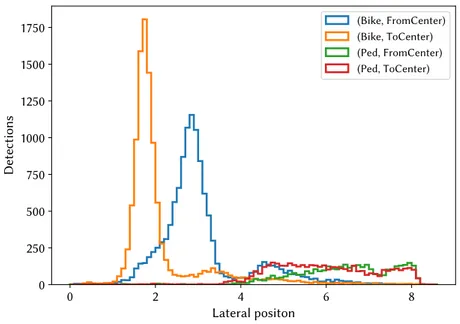
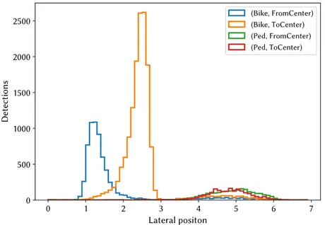
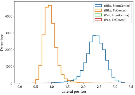
A Lateral distribution
Histograms of the distributions of lateral positions of the road users at the mea-surement cross sections are presented in fig. 4 to fig. 10. The bin width of the histograms is 10 cm. 0 1 2 3 4 Lateral positon 0 50 100 150 200 250 Detections (Bike, FromCenter) (Bike, ToCenter) (Ped, FromCenter) (Ped, ToCenter)
Figure 4: Distribution of the lateral position of the detected road users at the Danviksbron site.
0.0 0.5 1.0 1.5 2.0 2.5 3.0 Lateral positon 0 250 500 750 1000 1250 1500 1750 2000 Detections (Bike, FromUniv) (Bike, ToUniv) (Ped, FromUniv) (Ped, ToUniv)
Figure 5: Distribution of the lateral position of the detected road users at the Valla site. 0 2 4 6 8 Lateral positon 0 250 500 750 1000 1250 1500 1750 Detections (Bike, FromCenter) (Bike, ToCenter) (Ped, FromCenter) (Ped, ToCenter)
Figure 6: Distribution of the lateral position of the detected road users at the Ullevigatan site.
0 1 2 3 4 5 6 Lateral positon 0 200 400 600 800 1000 1200 Detections (Bike, FromCenter) (Bike, ToCenter) (Ped, FromCenter) (Ped, ToCenter)
Figure 7: Distribution of the lateral position of the detected road users at the Delsjövägen site. 0 1 2 3 4 5 6 7 Lateral positon 0 500 1000 1500 2000 2500 Detections (Bike, FromCenter) (Bike, ToCenter) (Ped, FromCenter) (Ped, ToCenter)
Figure 8: Distribution of the lateral position of the detected road users at the Liljeholmsbron site.
0.0 0.5 1.0 1.5 2.0 2.5 3.0 3.5 Lateral positon 0 1000 2000 3000 4000 Detections (Bike, FromCenter) (Bike, ToCenter) (Ped, FromCenter) (Ped, ToCenter)
Figure 9: Distribution of the lateral position of the detected road users at the Munkbroleden site. 0 1 2 3 4 Lateral positon 0 200 400 600 800 1000 1200 1400 1600 Detections (Bike, FromCenter) (Bike, ToCenter) (Ped, FromCenter) (Ped, ToCenter)
Figure 10: Distribution of the lateral position of the detected road users at the Strandvägen site.
B Flow distribution over time
The flow, aggregated over 30 min intervals are presented in fig. 11 to fig. 17.
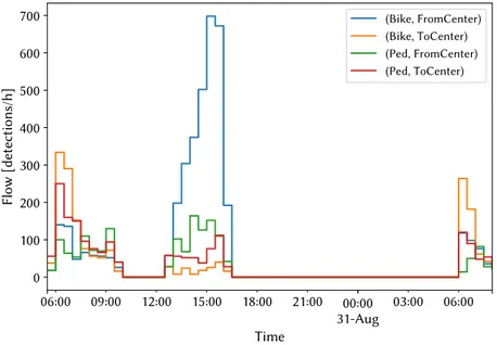
00:00 31-Aug 06:00 09:00 12:00 15:00 18:00 21:00 03:00 06:00 Time 0 100 200 300 400 500 600 700 Flow [detections/h] (Bike, FromCenter) (Bike, ToCenter) (Ped, FromCenter) (Ped, ToCenter)
21 01 Jun 2018 22 23 24 25 26 27 28 29 30 31 Time 0 100 200 300 400 500 Flow [detections/h] (Bike, FromUniv) (Bike, ToUniv) (Ped, FromUniv) (Ped, ToUniv)
Figure 12: Flows aggregated at the 30 min level at the Valla site.
04 Sep 2018 05 06 07 Time 0 100 200 300 400 500 600 Flow [detections/h] (Bike, FromCenter) (Bike, ToCenter) (Ped, FromCenter) (Ped, ToCenter)
04 Sep 2018 05 06 07 Time 0 100 200 300 400 500 Flow [detections/h] (Bike, FromCenter) (Bike, ToCenter) (Ped, FromCenter) (Ped, ToCenter)
Figure 14: Flows aggregated at the 30 min level at the Delsjövägen site.
18 Sep 2018 19 20 21 Time 0 200 400 600 800 1000 1200 Flow [detections/h] (Bike, FromCenter) (Bike, ToCenter) (Ped, FromCenter) (Ped, ToCenter)
18 Sep 2018 19 20 21 Time 0 250 500 750 1000 1250 1500 1750 Flow [detections/h] (Bike, FromCenter) (Bike, ToCenter) (Ped, FromCenter) (Ped, ToCenter)
Figure 16: Flows aggregated at the 30 min level at the Munkbroleden site.
18 Sep 2018 19 20 21 Time 0 200 400 600 800 Flow [detections/h] (Bike, FromCenter) (Bike, ToCenter) (Ped, FromCenter) (Ped, ToCenter)
C Volume – delay function
Total delay aggregated over one-minute intervals at each data set is presented in fig. 18 to fig. 26, together with the average delay at each flow level and the best fit quadratic volume delay function for each data set.
200 400 600 800 1000 1200 Volume −2.5 0.0 2.5 5.0 7.5 10.0 12.5 Delay [/km] Mean delay
aq
2Figure 18: Total delay aggregated at the one-minute level at the Danviksbron site during the afternoon peak in the direction from the city center.
200 400 600 800 1000 Volume −1 0 1 2 3 4 5 6 7 Delay [/km] Mean delay
aq
2Figure 19: Total delay aggregated at the one-minute level at the Ullevigatan site during the morning peak in the direction to the city center.
200 400 600 800 1000 1200 Volume 0 2 4 6 8 10 12 14 16 Delay [/km] Mean delay
aq
2Figure 20: Total delay aggregated at the one-minute level at the Ullevigatan site during the afternoon peak in the direction from the city center.
100 200 300 400 500 600 700 800 900 Volume 0.0 0.5 1.0 1.5 2.0 2.5 3.0 Delay [/km] Mean delay
aq
2Figure 21: Total delay aggregated at the one-minute level at the Delsjövägen site during the morning peak in the direction to the city center.
200 400 600 800 1000 1200 1400 1600 1800 Volume 0 5 10 15 20 Delay [/km] Mean delay
aq
2Figure 22: Total delay aggregated at the one-minute level at the Delsjövägen site during the morning peak in the direction to the city center.
500 1000 1500 2000 2500 Volume 0 5 10 15 20 25 30 Delay [/km] Mean delay
aq
2Figure 23: Total delay aggregated at the one-minute level at the Munkbroleden site during the morning peak in the direction to the city center.
200 400 600 800 1000 1200 1400 Volume 0 2 4 6 8 10 Delay [/km] Mean delay
aq
2Figure 24: Total delay aggregated at the one-minute level at the Munkbroleden site during the afternoon peak. in the direction from the city center
200 400 600 800 1000 1200 Volume 0 1 2 3 4 5 Delay [/km] Mean delay
aq
2Figure 25: Total delay aggregated at the one-minute level at the Strandvägen site during the morning peak in the direction to the city center.
200 400 600 800 1000 1200 Volume −2 0 2 4 6 8 10 Delay [/km] Mean delay
aq
2Figure 26: Total delay aggregated at the one-minute level at the Strandvägen site during the afternoon peak in the direction from the city center.