Climate Change Impacts on Water Resources of Greater Zab River, Iraq

(1)

doi: 10.17265/1934-7359/2016.12.009

Climate Change Impacts on Water Resources of Greater

Zab River, Iraq

Nahlah Abbas1, Saleh A. Wasimi1 and Nadhir Al-Ansari2

1. School of Engineering and Technology, Central Queensland University, Melbourne 3000, Australia 2. Geotechnical Engineering, Lulea University of Technology, Lulea 971 87, Sweden

Abstract: Greater Zab is the largest tributary of the Tigris River in Iraq where the catchment area is currently being plagued by water scarcity and pollution problems. Contemporary studies have revealed that blue and green waters of the basin have been manifesting increasing variability contributing to more severe droughts and floods apparently due to climate change. In order to gain greater appreciation of the impacts of climate change on water resources in the study area in near and distant future, SWAT (Soil and Water Assessment Tool) has been used. The model is first tested for its suitability in capturing the basin characteristics, and then, forecasts from six GCMs (general circulation models) with about half-a-century lead time to 2046~2064 and one-century lead time to 2080~2100 are incorporated to evaluate the impacts of climate change on water resources under three emission scenarios: A1B, A2 and B1. The results showed worsening water resources regime into the future.

Key words: Greater Zab, SWAT, sensitivity, blue water, green water.

1. Introduction

The water resources of a basin is impacted by a multitude of variables such as precipitation and other meteorological factors, vegetation and other land use, natural calamities such as hurricanes, and induced catastrophes such as bushfires. Changes in climate, population and land use have profound impacts on the supply and demand balance of future water resources and water availability at a global [1, 2] and regional scale [3, 4]. Where the water resources are limited, the water balance is often delicate and the situation can easily aggravate by climate change [5] which can be unprecedented because the water system is vulnerable to climate change outside the range of historical events [6]. Climate change can considerably impact on the hydrological cycles mainly through the alteration of evapotranspiration and precipitation [7-9]. The effects can strikingly manifest as severe droughts or raging floods having a profound impact on the water balance

Corresponding author: Saleh A. Wasimi, associate professor, research fields: water resources planning and management and hydrology.

of a basin [10].

Countries in the middle-east typically suffer from water shortages and the long-term predictions are rather ominous—more water shortages in both surface and groundwater resources in the future [11, 12]. Iraq fits the description of a typical middle-east country, and it is highly vulnerable to climate change [13]. The country can be classified as arid or semi-arid with less than 150 mm of annual rain and high evaporation rate. Its water balance is rather delicate threatened by water scarcity that can significantly exacerbate due to climate change [12, 13]. Arguably, climate change is one of the greatest challenges confronting Iraq, its adverse effects on water resources can alter the environment and impact the economy, particularly the agricultural sector. Understandably, therefore, there is a strong demand from decision makers for predictions about the potential impacts of climate change on the duration and magnitude of precipitation, which have ramifications on sustaining and managing water resources appropriately and alleviating water scarcity problem that has become pronounced [12].

In northern Iraq, Greater Zab is the largest tributary

D

(2)

of Tigris River in terms of its contribution to Tigris flow. Based on some estimates, Greater Zab contributes around 40%~60% of total Tigris flow [14]. Further, it is the only source of surface water for Erbil City, the capital of Iraqi Kurdistan. This basin has been suffering from water scarcity and pollution [15]. So far, water issues related to climate change in the Greater Zab catchment have not been well addressed within climate change analyses and climate policy construction [16]. Therefore, the main objective of this study has been to assess the potential future climatic changes on the water sources of Greater Zab, specifically blue and green waters. The computer-based hydrological model SWAT (Soil and Water Assessment Tool) has been used to explore the effects of climatic change on stream flow of the study area. The model was set at monthly scale using available spatial and temporal data and calibrated against measured stream flow. Climate change scenarios were obtained from general circulation models.

2. Materials and Methods

2.1 Study Area

Greater Zab originates from the Ararat Mountains in

Turkey, runs through the central northern part of Iraq, and then, links with Tigris River south of Mosul City traversing a distance of 372 km (Fig. 1). Greater Zab and its tributaries namely Shamdinan, Haji Beg, Rawandooz and Khazir-Gormal rivers are located between latitudes 36° N and 38° N, and longitudes 43.3° E and 44.3° E [15]. It drains an area of 26,473 km2, 65% of which is located in Iraq and the remainder in Turkey [12]. Greater Zab basin is a mountainous area with elevation ranging from 180 m to 4,000 m above sea level (Fig. 1). There are many springs in the basins which are the main source for irrigation [17]. Mean annual temperature is 14.3 °C and mean annual precipitation is 570 mm, ranging from 350 mm to 1,000 mm. Most of the precipitation in the Greater Zab basin falls in winter and spring. Typically, the rainfall is distributed over the year: 48.9% including snowfall falls in winter, 37.5% in spring, 12.9% in autumn, and 0.57% in summer [17].The flow regime of Greater Zab demonstrates highly seasonal flow with peak flow occurring in May and low seasonal flow from July to December. This is a typical near-natural nival regime, in which winter precipitation in the form of snow and snow-melt in the spring is dominant. So far no dam has been constructed

(a) (b) Fig. 1 Greater Zab basin: (a) the location; (b) DEM (digital elevation model).

(3)

on the river, however, both countries (Turkey and Iraq) have plans to build dams on the river [14]. Seventy nine percent of the watershed is covered by pasture, and 21% of the land is used for different agricultural activities. There are three discharge stations namely, Bekhme, Bakrman and EskiKelek stations. Bekhme station lies at latitude 36.63° N and longitude 44.48° E, northeast of the basin. Bakrman station is located near the Greater Zab outlet, at latitude 36.33° N and longitude 43.55° E at Khazir River, one of Greater Zab’s tributaries. EskiKelek station is situated in the lower part of the basin, at the basin outlet, at latitude 36° N and longitude 43.35_{° E.}

2.2 Description of SWAT model

SWAT [18] is a river watershed scale, semi-distributed, and physically based continuous time (daily computational time step) mathematical model for analyzing hydrology and water quality at various watershed scales with varying soils, land use and management conditions on a long-term basis. The SWAT model was originally developed by the USDA (United States Department of Agriculture) and the ARS (Agricultural Research Service) at the Grassland, Soil and Water Research Laboratory in Temple, Texas, USA [19]. SWAT system is embedded within a geographic information system (ArcGIS interface), in which different spatial environmental data, including climate, soil, land cover and topographic characteristics can be integrated.

Two major divisions, land phase and routing phase, are conducted to simulate the hydrology of a watershed. The land phase of the hydrological cycle predicts the hydrological components including surface runoff, evapotranspiration, groundwater, lateral flow, ponds, tributary channels and return flow. The routing phase of the hydrological cycles is the movement of water, sediments, nutrients and organic chemicals via the channel network of the basin to the outlet [18]. In the land phase of the hydrological cycle, the simulation of

the hydrological cycle is based on the water balance equation: ܹܵ_௧ൌ ܹܵ_଴൅ ෍൫ܴ_ௗ௔௬െ ܳ_௦௨௥௙െ ܧ_௔ ௡ ௜ୀଵ െ ܹ_௦௘௘௣െ ܳ_௚௪ሻ (1) where, SWt is the final soil water content (mm), SWo is

the initial soil water content on day i (mm), t is the time (days), Rday is the amount of precipitation on day i

(mm), Qsurf is the amount of surface runoff on day i

(mm), Ea is the amount of evapotranspiration on day i

(mm), Wseep is the amount of water entering the vadose

zone from the soil profile on day i (mm), and Qgw is the

amount of return flow on day i (mm).

The SWAT model enables users to estimate surface runoff through two methods; the SCS (soil conservation service) curve number procedure (SCS 1972 in Ref. [18] and the Green and Ampt infiltration method [20]). The SCS method has been used in this study due to non-availability of sub-daily data that is required by the Green and Ampt infiltration method. The model estimates the volume of lateral flow depending on the variation in conductivity, slope and soil water content. A kinematic storage model is utilized to predict lateral flow through each soil layer. Lateral flow occurs below the surface when the water rates in a layer exceed the field capacity after percolation. The groundwater simulation is divided into two aquifers which are a shallow aquifer (an unconfined) and a deep confined aquifer in each watershed. The shallow aquifer contributes to stream flow in the main channel of the watershed. Water that percolates into the confined aquifer is presumably contributing to stream flow outside the watershed. Three methods are provided by SWAT model to estimate potential evapotranspiration (PET); the Penman-Monteith method [21], the Priestley-Taylor method [22] and the Hargreaves method [23]. The Penman-Monteith method requires air temperature, wind-speed, solar radiation and relative humidity; Priestley-Taylor method needs air temperature and solar radiation, while Hargreaves method needs only daily temperature as inputs. Water

(4)

is routed through the channel network by applying either the variable storage routing or Muskingum River routing methods using the daily time step.

2.3 Model Input

Enormous amount of input data is required by SWAT to fulfill the tasks envisaged in this research. Basic data requirements for modelling include DEM (digital elevation model), land use map and soil map, weather data and discharge data. DEM was extracted from ASTER Global Digital Elevation Model (ASTERGDM) with a 30 m grid and 1 × 1 degree tiles.1_{The land cover map was obtained from the} European Environment Agency2 with a 250 m grid raster for the year 2000. The soil map was collected from the global soil map of the Food and Agriculture Organization of the United Nations [24]. Weather data which includes daily precipitation, 0.5 hourly precipitations, maximum and minimum temperatures were obtained from the Iraq’s Bureau of Meteorology. Monthly stream flow was collected from the Iraqi Ministry of Water Resources/National Water Centre.

2.4 Model Setup

In SWAT, the watershed is divided into sub-basins based on the DEM. The land use map, soil map and slope datasets are embedded with the SWAT databases. Thereafter, sub-basins are further delineated by HRUs (hydrologic response units). HRUs are defined as packages of land that have a unique slope, soil and land use area within the borders of the sub-basin. HRUs enable the user to identify the differences in hydrologic conditions such as evapotranspiration for varied soils and land uses. Routing of water and pollutants are predicted from the HRUs to the sub-basin level and then through the river system to the watershed outlet.

2.5 Model Calibration and Validation

2.5.1 SUFI-2 Algorithm Description

1_{http://gdem.ersdac.jspacesystems.or.jp/tile_list.jsp.}

2_{http://www.eea.europa.eu/data-and-maps/data/global-land-cov}

er-250m.

To evaluate the performance of SWAT, the sequential uncertainty fitting algorithm application (SUFI-2) embedded in the SWAT-CUP package [25] was used. The advantages of SUFI-2 are that it combines optimization and uncertainty analysis, can handle a large number of parameters through Latin hypercube sampling, and it is easy to apply [25]. Furthermore, as compared with other different techniques used in SWAT such as generalized GLU (likelihood uncertainty estimation), parameter solution (parsol), MCMC (Markov chain Monte Carlo), SUFI-2 algorithm was found to obtain good prediction uncertainty ranges with a few number of runs [26]. This efficiency is of great significance when implementing complex and large-scale models [27].

The SUFI-2 first identifies the range for each parameter. After that, Latin hypercube method is used to generate multiple combinations among the calibration parameters. Finally, the model runs with each combination and the obtained results are compared with observed data until the optimum objective function is achieved. Since the uncertainty in forcing inputs (e.g., temperature, rainfall), conceptual model and measured data are not avoidable in hydrological models, the SUFI-2 algorithm computes the uncertainty of the measurements, the conceptual model and the parameters by two measures: P-factor and R-factor. P-factor is the percentage of data covered by the 95% PPU (prediction uncertainty) which is quantified at 2.5% and 97.5% of the cumulative distribution of an output variable obtained through Latin hypercube sampling [25]. The R-factor is the average width of the 95 PPU divided by the standard deviation of the corresponding measured variable. In an ideal situation, P-factor tends towards 1 and

R-factor to zero [25]. The objective of the algorithm is

to increase P-factor and reduce R-factor in order to achieve the optimal parameter range. These factors together reflect the strength of the calibration-uncertainty analysis. Further, SUFI-2 calculates the coefficient of determination (R2) and the

(5)

ENC (Nasch-Sutcliff efficiency) [28] to assess the goodness of fit between the measured and simulated data. R2_{shows the strength of the relationship between} the simulated and observed data. It ranges from 0 to 1 [29]. The higher values of R2 reflect less error variance, and values greater than 0.5 are satisfactory [30]. R2 has been widely used to provide an assessment of climate change detection, hydrological and hydroclimatological applications [29, 31, 32]. R2 is given by ܴଶ_{ൌ ቈ} σ௡௜ୀଵሺܱ௜െ ܱതሻሺܲ௜െ ܲതሻ ሾσ௡௜ୀଵሺܱ௜െ ܱതሻଶሿ଴Ǥହሾσ௡௜ୀଵሺܲ௜െ ܲതሻଶሿ଴Ǥହ ቉ ଶ (2) where, Oi is the observed stream flow, Pi is the

simulated stream flow, ƿ is the mean observed stream flow during the evaluation period and ܲത is the mean simulated stream flow for the same period.

The ENC value is an indication of how well the plot of the observed against the simulated values fits the 1:1 line. It can range from negative infinity (-) to one. The closer the value to one, the better the prediction is, while the value of less than 0.5 indicates unsatisfactory model performance [30]. ENC is calculated as shown below: ܧܰܥ ൌ ͳ െ ቈσ ሺܱ௜െ ܲ௜ሻଶ ௡ ௜ୀଵ σ௡ ሺܱ_௜െ ܱതሻଶ ௜ୀଵ ቉ (3)

ENC was recommended to be used for calibration

for two reasons. First, it has been adopted by ASCE [33] and second, Gegates et al. [29] recommend it due to its straightforward physical interpretation [34]. Besides, it has found wide applications offering extensive information on reported values [31].

SUFI-2 enables users to conduct global sensitivity analysis, which is computed based on the Latin hypercube and multiple regression analysis. The multiple regression equation is defined as below:

݃ ൌ ߙ ൅ ෍ ߚ_௜כ ܾ_௜ ௠

௜ୀଵ

(4) where, g is the value of evaluation index for the model simulations, Į is a constant in multiple linear regression equation, ȕ is the coefficient of the regression equation,

b is a parameter generated by the Latin hypercube

method and m is the number of parameters.

The t-stat of this equation which indicates parameter sensitivity is applied to determine the relative significance for each parameter [35], the more the sensitive parameter, the greater is the absolute value of the t-stat [25]. P-value is an indication of the significance of the sensitivity, P-value close to zero has more significance.

2.6 GCM (General Circulation Model) inputs

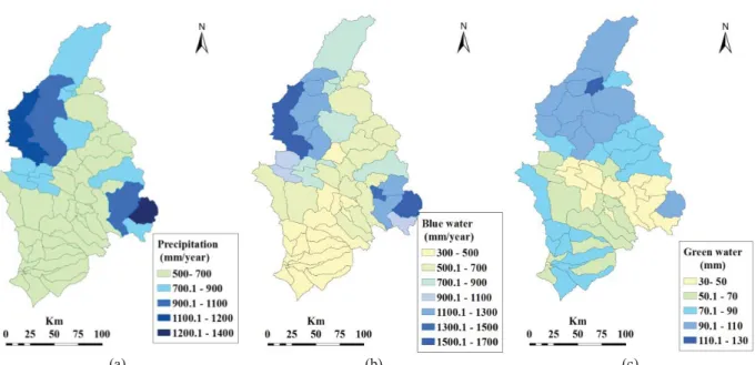
Six GCMs from CMIP3 namely CGCM3.1/T47, CNRM-CM3, GFDL-CM2.1, IPSLCM4, MIROC3.2 (medres) and MRI CGCM2.3.2 were selected for climate change projections in the Lesser Zab basin under a very high emission scenario (A2), a medium emission scenario (A1B) and a low emission scenario (B1) for two future periods (2046~2064) and (2080~2100). The projected temperatures and precipitation were then inputted to the SWAT model to compare water resources in the basin with the baseline period (1980~2010). Fig. 2 captures the outputs from the models, where blue water refers to freshwater in rivers, lakes, and aquifers and green water refers to the part of precipitation that is held by soil and vegetation which eventually returns to atmosphere through evapotranspiration. BCSD method was used to downscale the GCM results [36].

3. Results and Discussion

3.1 Sensitivity Analysis

Sensitivity analysis has been carried out for 25 parameters related to stream flow (Table 1), from which 12 most sensitive parameters have been considered, as is the usual practice, for implementing model calibration for the Greater Zab basin.

The ranking of 12 highest sensitive parameters for the watershed is presented in Table 2. For Greater Zab,

SFTMP was the most sensitive parameter. This is

(6)

(a) (b) (c)

Fig. 2 For the baseline period of 1980~2010: (a) average of precipitation; (b) average of blue water; (c) average of green water storage.

Table 1 Description of input parameters of stream flow selected for model calibration.

Group Parameter Description Unit

Soil

SOL_ALB Moist soil albedo -

SOL_AWC Available water capacity mm·mm-1

SOL_K Saturated hydraulic conductivity mm·h-1

SOL_Z Depth to bottom of second soil layer mm

Groundwater

ALPHA_BF Base flow alpha factor day

GW_DELAY Groundwater delay day

GW_REVAP Groundwater “revap” coefficient -

GWQMN Threshold depth of water in the shallow aquifer for return flow to occur mm·H2O

REVAPMN Threshold depth of water in the shallow aquifer for “revap” to occur mm·H2O

Subbasin TLAPS Temperature laps rate °C·km–1

HRU

EPCO Soil evaporation compensation factor -

ESCO Plant uptake compensation factor -

CANMX Maximum canopy storage mm·H2O

SLSUBBSN Average slope length m

Routing CH_N2 Manning’s n value for the main channel -

CH_K2 Effective hydraulic conductivity in main channel alluvium mm·h–1

Management BIOMIX Biological mixing efficiency -

CN2 Initial SCS runoff curve number for moisture condition II -

General data basin

SFTMP Snowfall temperature °C

SMFMN Minimum melt rate for snow during year mm·H2O·°C–1·day–1

SMFMX Maximum melt rate for snow during year mm·H2O·°C–1·day–1

TEMP Snow pack temperature lag factor -

SURLAG Surface runoff lag time day

BLAI Maximum potential leaf area index for land cover/plant -

(7)

Table 2 Ranking of 12 highest sensitive parameters related to stream flow in the two basins.

Parameter Ranking Initial values Fitted values

SFTMP 1 -5~5 3.5475 ALPHA_BF 2 0~1 0.032500 CN2 3 -0.2~0.2 -0.175 SOL_AWC 4 -0.2~0.4 0.052 HRU_SLP 5 0~0.2 0.05650 SLSUBBSN 6 0~0.2 0.15450 SURLAG 7 0.05~24 17.4 ESCO.hru 8 0~0.2 0.85850 GWQMN 9 0~2 1.155000 CH_K2 10 5~130 76.87 GW_REVAP 11 0~0.2 0.179500 GW_DELAY 12 30~450 35.25 (a) (b) Fig. 3 The SWAT model at monthly scale at Bekame station: (a) calibration; (b) validation. mountainous basin. Among the groundwater related

parameters, ALPHA-BE was observed to be the most sensitive parameter which was ranked as the second. This result is consistent with the finding of Li et al. [37], who found that ALPHA is a highly sensitive groundwater parameter during SWAT calibration. CN2 was ranked the third. In most SWAT applications in different watersheds, CN2 was found to be the most sensitive parameter [38]. SOL_AWC came the fourth.

3.2 Calibration and Validation

SWAT was calibrated and validated for Greater Zab basin at three discharge stations on a monthly scale (Bekhme station, Bakrmanstation and EskiKelek station). The model was calibrated for 18 years (1979~1996) and validated for 8 years (1997~2004),

the first three years was set as a warm up.

The results of monthly discharge calibration and validation for the three stations showed good agreement with observed data as shown in Figs. 3-5. The highest R2_{and ENC were obtained for EskiKelek} Station during the calibration and validation processes (Fig. 5), where R2 and ENC were 0.77 and 0.70, respectively, during the calibration. R2 increased to 0.89 and ENC decreased to 0.66 during the validation. This is because of the fact that EskiLelek station is located at the outlet of the basin and the model is calibrated from upstream to downstream [25]. The calibrated parameters of upstream stations contribute partially to the calibration process of downstream stations [26], thus enhancing simulation results of downstream EskiKelek station.

0 500 1000 1500 2000 2500

Jan-82 Jul-82 Jan-83 Jul-83 Jan-84 Jul-84 Jan-85 Jul-85 Jan-86 Jul-86 Jan-87 Jul-87 Jan-88 Jul-88 Jan-89 Jul-89 Jan-90 Jul-90 Jan-91 Jul-91 Jan-92 Jul-92 Jan-93 Jul-93 Jan-94 Jul-94 Jan-95 Jul-95 Jan-96 Jul-96

Discharge (m 3/s) Time-Monthly Calibration _95PPU observed Best_Sim R2_=0.69 ENC=0.66 P-factor=0.77 R-factor=1.08 0 200 400 600 800 1000 1200 1400 1600 1800

Jan-97 Jul-97 Jan-98 Jul-98 Jan-99 Jul-99 Jan-00 Jul-00 Jan-01 Jul-01 Jan-02 Jul-02 Jan-03 Jul-03 Jan-04 Jul-04

Discharge (m 3/sec) Time-Monthly Validation 95PPU observed Best_Sim R2_=0.84 ENC=0.53 P-factor=0.51 R-factor=1.34

(8)

(a) (b) Fig. 4 The SWAT model at monthly scale at Bakrman station: (a) calibration; (b) validation.

Fig. 5 The SWAT model at monthly scale at EskiKelek: (a) calibration; (b) validation. 3.2.1 Trends in Precipitation, Blue Water, Green

Water, Storage and Water Flow in the Past

Using the calibrated model, annual precipitation, blue water (summation of water yield and deep aquifer recharge) and green water storage (soil water content) and green water flow (evapotranspiration) were estimated during the last three decades to identify the impacts of climate change on the water cycle components. Blue water is the freshwater humans can access for instream use or withdrawal. Green water storage does not provide direct access to humans but sustains natural flora and rain-fed agriculture. Green water flow is actual evapotranspiration. The model outputs matched observations.

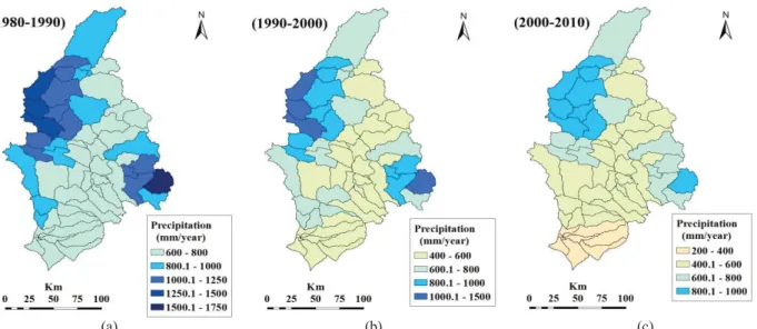
Fig. 6 captures the spatial distribution of precipitation in HRUs over three consecutive decades. Generally, precipitation decreased from upstream to downstream and from the east to the west of the basin. This is because the upper and east part of the basin is mountainous, experiencing higher precipitation and snowfall compared to the lower and western part of the basin which is rather flat and experiencing less snowfall. From Fig. 6, it is apparent that there is a general declining trend in precipitation over time. The 1990s and 2000s decades experienced decreases by about 21% and 32% compared to 1980s decade, respectively (Table 3). 0 20 40 60 80 100 120

Discharge (m 3/sec) Time-Monthly Calibration 95PPU observed Best_Sim R2_=0.53 ENC=0.55 P-factor=0.58 R-factor=0.88 0 10 20 30 40 50 60 70 80

Discjharge (m 3/sec) Time-Monthly Validation 95PPU observed Best_Sim R2_=0.66 ENC=0.52 P-factor=0.89 R-factor=1.76 0 500 1000 1500 2000 2500 3000

Discharge (m 3 / sec) Time-Monthly 995PPU observed Best_Sim R2_{= 0.77} ENC= 0.70 P-factor= 0.76 R-factor= 1.23 Calibration 0 200 400 600 800 1000 1200 1400 1600 1800 2000

Discharge (m 3/sec) Time-Monthly Validation 95PPU observed Best_Sim R2_=0.89 ENC=0.66 P-factor=0.81 R-factor=0.92

(9)

(a) (b) (c)

Table 3 Relative changes in precipitation, blue water and green water in the Lesser Zab basin over three decades. Water component Rate of relative change in the last three decades

1990s vs. 1980s 2000s vs. 1990s 2000s vs. 1980s

Precipitation -0.21 -0.14 -0.32

Blue water -0.29 -0.25 -0.46

Green water storage -0.12 -0.06 -0.17

Green water flow -0.06 -0.04 -0.05

(a) (b) (c) Fig. 7 Spatial distribution of blue water in the Greater Zab basin over three consecutive decades.

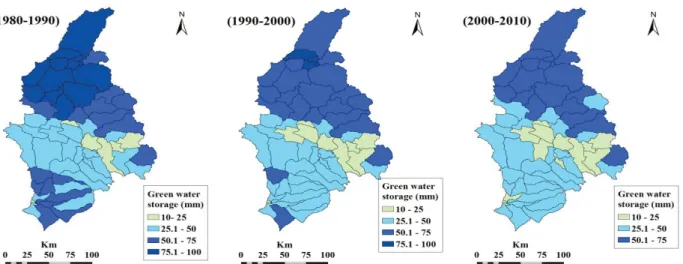
Blue water and green water storage in the Greater Zab basin decreased from upstream to downstream (Figs. 7 and 8). Generally, green water tracks blue water, where blue water flows are high, green water flows also have a tendency to be high. The spatial patterns

of the blue and green water flows are largely influenced by the spatial patterns of precipitation. Land cover also influences the forming of spatial patterns. The average annual blue water and green water storage for the entire catchment significantly

(10)

decreased from 1980s to 2000s. It is possible that the decreasing trends in the average annual blue water and green water are attributable to climate change. Green water flow was relatively stable during the entire period (Table 3) due to the assumption that land cover/land use remained unchanged during the period of 1980 to 2010.

3.3 Blue Water Scarcity Indicators

The calibrated model was used for water scarcity analysis. Among a large number of water scarcity indicators, the most widely applied and accepted is the

water stress threshold [39], defined as 1,700 m3·capita-1·year-1 introduced by Falkenmark [40],

which was used in this study. The 1,700 m3·capita-1·year-1 is calculated based on estimations of water needs in the household, agriculture, industry and energy sectors, and the demand of the environment [39]. A value equal or greater than 1,700 m3_·capita-1_·year-1_{is considered as} adequate to meet water demands. When water supply drops below 1,000 m3·capita-1·year-1, it is referred to as water scarcity and below 500 m3·capita-1·year-1 is extreme scarcity. The water availability per capita and water stress indicators were estimated for each of the 61 sub-basins of the Greater Zab catchment using the 2.5 arcmin population map available from the CIESIN

(Center for International Earth Science) Gridded Population of the World (GPW, version 3)3_{for 2005.} Fig. 9 demonstrates the spatial distribution of water resources per capita per year during the period of 1980~2010 based on the population estimates of the year of 2005. In general, up to 55% of the basin area, mostly located in the lower part of the basin, experienced extreme water scarcity. Twenty four percent of the basin experienced between 1000 m3 and 500 per capita per year. Seven percent only experienced sufficient blue water located in the upper part of the basin.

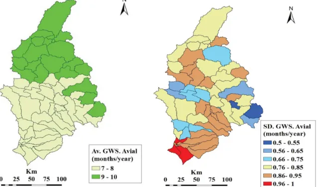
3.3.1 Uncertainty and Natural Variation in Green Water Storage

For the rain-fed agriculture, the average of the months per year for the period of 1980 to 2010 where green water storage is available (defined as > 1 mm·m-1₎ is of greatest importance [41]. This is shown in Fig. 10a—up to 65% of the basin experienced 7 to 8 months (October to May) in which green water was not depleted. The standard deviation (SD) of the months per year without depleted soil water is presented for the 1980~2010 period in Fig. 10b. The areas with a high SD such as the lower part of the basin show high variability in green water storage availability.This mayresultin reducedcrop yield. In

(11)

Fig. 9 Water scarcity in each modeled Greater Zab sub-basin represented by the modeled 1980 to 2010 annual average blue water flow availability per capita per year (using population of 2005) the average (Avg.) value of the 95PPU range.

Fig. 10 The number of months per year where the GW-S (green water storage)is available for usage: (a) the 1980~2010 average (Av.); (b) standard deviation (SD).

(12)

order to sustain agriculture production in this part, adjusting irrigation systems and alternative cropping practices are highly recommended.

3.4 The Impacts of Climate Change on Temperature and Precipitation

Mean annual temperature and precipitation outputs from the six GCMs identified earlier were processed for the Greater Zab basin under three scenarios (A2, A1B, B1). Table 4 captures the projected changes in mean annual temperature for two future periods (2046~2064) and (2080~2100) relative to base period (1980~2010). Changes in mean temperature tend to be more consistent than precipitation. All the models showed steady increasing trends in temperature. GFDL (Geophysical Fluid Dynamics Laboratory) model projected the highest increases in mean temperature; however MRI (Meteorological Research Institute) predicted the lowest increases. Mean

temperature of six models would increase by about 2.6 °C, 2.2 °C and 1.3 °C under A2, A1B and B1, respectively, for near future (2046~2064). For distant future, the mean temperature would increase by 5 °C, 4.3 °C and 1.55 °C for A2, A1B and B1 scenarios, respectively. Changes in mean temperature modify evapotranspiration and precipitation and hence blue water and green water flows.

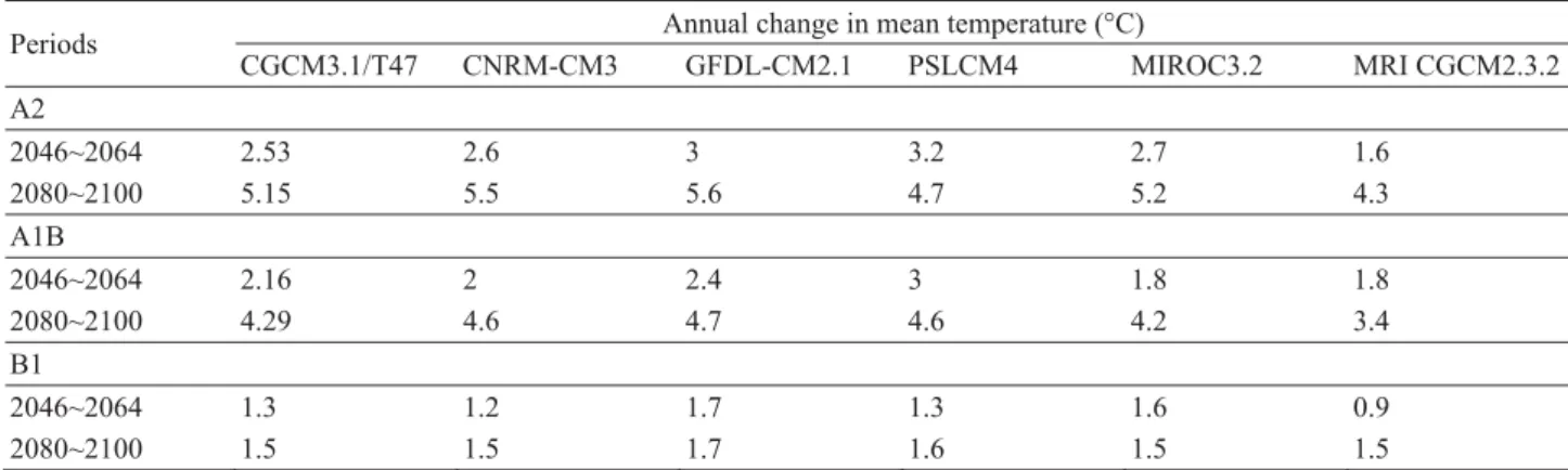
Generally, all models showed a decrease in mean annual precipitation at half-a-century future (2046~2064) and one-century future (2080~2100) except MRI CGCM2.3.2. GFDL yielded highest decreases (Table 5). Fig. 11 shows the anomaly maps of precipitation distribution (maps of percent deviation from historic data, 1980~2010) for A2, A1B and B1 scenarios for the periods 2046~2064 and 2080~2100 for the average change of multi-GCM ensemble. A2 emission scenario produced the highest decreases while B1 emission scenario gave the lowest reductions Table 4 GCM predicted changes in the mean annual temperature of the future under A2, A1B and B1 scenarios.

Periods Annual change in mean temperature (°C)

CGCM3.1/T47 CNRM-CM3 GFDL-CM2.1 PSLCM4 MIROC3.2 MRI CGCM2.3.2 A2 2046~2064 2.53 2.6 3 3.2 2.7 1.6 2080~2100 5.15 5.5 5.6 4.7 5.2 4.3 A1B 2046~2064 2.16 2 2.4 3 1.8 1.8 2080~2100 4.29 4.6 4.7 4.6 4.2 3.4 B1 2046~2064 1.3 1.2 1.7 1.3 1.6 0.9 2080~2100 1.5 1.5 1.7 1.6 1.5 1.5

Table 5 GCM predicted changes in the mean annual precipitation of the future under A2,A1B and B1 scenarios.

Periods Annual change in precipitation (%)

CGCM3.1/T47 CNRM-CM3 GFDL-CM2.1 PSLCM4 MIROC3.2 MRI CGCM2.3.2 A2 2046~2064 -0.19 -0.28 -0.18 -0.18 -0.18 0.012 2080~2100 -0.22 -0.12 -0.35 -0.26 -0.28 -0.11 A1B 2046~2064 -0.03 -0.10 -0.17 -0.15 -0.11 0 2080~2100 -0.09 -0.18 -0.25 -0.23 -0.22 0.13 B1 2046~2064 0.02 -0.04 -0.07 -0.14 -0.10 0.09 2080~2100 -0.09 -0.06 -0.15 -0.05 -0.07 0.04

(13)

(a) (b)

(c) (d)

(e) (f)

Fig. 11 The impacts of climate change on the precipitation of the basin: (a) anomaly based on Scenario A2 for the period of 2046~2064; (b) anomaly for A2 to 2080~2100; (c) anomaly for A1B to 2046~2064; (d) anomaly for A1B to 2080~2100; (e) Anomaly for B1 to 2046~2064; (f) anomaly for B1 to 2080~2100.

(14)

(a) (b)

(c) (d)

(e) (f)

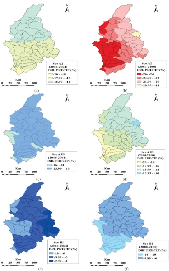
Fig. 12 The impacts of climate change on the blue water of the basin: (a) anomaly based on Scenario A2 for the period of 2046~2064; (b) anomaly for A2 to 2080~2100; (c) anomaly for A1B to 2046~2064; (d) anomaly for A1B to 2080~2100; (e) anomaly for B1 to 2046~2064; (f) anomaly for B1 to 2080~2100.

(15)

(a) (b)

(c) (d)

(e) (f)

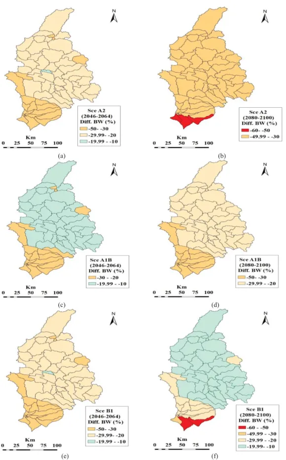
Fig. 13 The impacts of climate change on the green water storage of the basin: (a) anomaly based on Scenario A2 for the period of 2046~2064; (b) anomaly for A2 to 2080~2100; (c) anomaly for A1B to 2046~2064; (d) anomaly for A1B to 2080~2100, (e) anomaly for B1 to 2046~2064; (f) anomaly for B1 to 2080~2100.

(16)

(a) (b)

(c) (d)

(e) (f)

Fig. 14 The impacts of climate change on the deep aquifer recharge of the basin: (a) anomaly based on Scenario A2 for the period of 2046~2064; (b) anomaly for A2 to 2080~2100; (c) anomaly for A1B to 2046~2064; (d) anomaly for A1B to 2080~2100; (e) anomaly for B1 to 2046~2064; (f) anomaly for B1 to 2080~2100.

(17)

for both periods. The half-century projection (2046~2064) will experience average decreases of 16%, 12% and 5% under A2, A1B and B1 scenarios, respectively. In the one-century future, the reductions will increase to 22%, 16% and 10% under A2, A1B and B1 scenarios, respectively.

The reductions in the lower and the west part of the basin would be quite large, as high as 20% and 26% for the half-century future and one-century future, respectively, under extreme A2 emission scenario. As these parts are experiencing low precipitation, the projected decreases could have significant effects on frequent droughts and hence on agricultural productions.

3.5 Impacts of Climate Change on Blue and Green Water Flows

Fig. 12 captures the anomaly maps of blue water distribution (maps of percent deviation from historic data, 1980~2010) for A2, A1B and B1 scenarios for the periods 2046~2064 and 2080~2100 for the average change of multi-GCM ensemble. The half-century projection (2046~2064) will see a decrease in blue water under all emission scenarios for the whole basin. A2 scenario projected the highest reduction (29%) followed by A1B (20%) and then B1 (12%). In the one-century future, the reduction will increase to 38%, 29% and 20% under A2, A1B and B1 emission scenarios, respectively. Similarly, green water storage will decrease under the three emission scenarios for the two future periods, which is captured in Fig. 13. Green water flow calculations (maps not shown) indicated a slight decrease in evapotranspiration due to assumption that land cover would not significantly change from the period of 1980 to 2010 in the future.

4. Conclusions

The model, SWAT was applied to the Greater Zab basin at monthly time steps. The model was calibrated and validated at three discharge stations to simulate

the stream flow. The performance of the model was found to be satisfactory with R2_{and ENC indices} during the calibration and validation periods. The calibrated model was used for identifying the trends of water components in the last three decades. Precipitation, blue water, and green water flows were found to significantly decrease from 1980 to 2010. The findings matched with observations. Next, the model was applied for assessing the impacts of climate change in near and distant futures under three emission scenarios (A2, A1B, B1) using six GCMs. All models run under three emission scenarios predicted that the catchment will be drier in the near and distant futures. The results of this study could be beneficial in identifying appropriate water resources management strategies and cultivation practices of the future.

References

[1] Arnell, N. W., Vuuren, D. P., and Isaac, M. 2011. “The Implications of Climate Policy for the Impacts of Climate Change on Global Water Resources.” Global

Environmental Change 21: 592-603.

[2] Beck, L., and Bernauer, T. 2011. “How Will Combined Changes in Water Demand and Climate Affect Water Accessibility in the Zambezi River Basin?.” Global

Environmental Change 21: 1061-72.

[3] Tong, S. T. Y., Sun ,Y., Ranatunga, T., He, J., and Yang, Y. J. 2012. “Predicting Plausible Impacts of Sets of Climate and Land Use Change Scenarios on Water Resources.”

Applied Geography 32: 477-89.

[4] Gallart, F., Delgado, J., Beatson, S. J. V., Posner, H., Llorens, P., and Marcé, R. 2011. “Analyzing the Effect of Global Change on the Historical Trends of Water Resources in the Headwaters of the Llobregat and Ter River Basins (Catalonia, Spain).” Physics and Chemistry

of the Earth 36: 655-61.

[5] Tabari, H., and Willems, P. 2016. “Daily Precipitation Extremes in Iran: Decadal Anomalies and Possible Drivers.” Journal of American Water Resources

Association 52: 541-99.

[6] Borgomeo, E., Pflug, G., Hall, J. W., and Hochrainer-Stigler, S. 2015. “Assessing Water Resource System Vulnerability to Unprecedented Hydrological Drought Using Copulas to Characterize Drought Duration and Deficit.” Water Resources Research 51: 8927-48.

(18)

[7] Mimikou, M. A., Baltas, E., Varanou, E., and Pantazis, K. 2000. “Regional Impacts of Climate Change on Water Resources Quantity and Quality Indicators.” Journal of

Hydrology 234: 95-109.

[8] Winter, J. M., and Eltahir, E. A. B. 2012. “Modeling the Hydroclimatology of the Midwestern United States. Part 1: Current Climate.” Climate Dynamics 38: 573-93. [9] Xuan, Z., and Chang, N. B. 2014. “Modeling the

Climate-Induced Changes of Lake Ecosystem Structure under the Cascade Impacts of Hurricanes and Droughts.”

Ecological Modelling 288: 79-93.

[10] Owor, M., Taylor, R. G., Tindimugaya, C., and Mwesigwa, D. 2009. “Rainfall Intensity and Groundwater Recharge: Empirical Evidence from the Upper Nile Basin.”

Environmental Research Letters 4: 035009.

[11] Chenoweth, J., Hadjinicolaou, P., Bruggeman, A., Lelieveld. J., Levin, Z., Lang, M. A., Xoplaki, E., and Hadjikakou, M. 2011. “Impact of Climate Change on the Water Resources of the Eastern Mediterranean and Middle East Region: Modeled 21st Century Changes and Implications.” Water Resources Research 47: 1-18. [12] Al-Ansari, N., Ali, A. A., and Knutsson S. 2014. “Present

Conditions and Future Challenges of Water Resources Problems in Iraq.” Journal of Water Resource and

Protection 6: 1066-98.

[13] IPCC (Intergovernmental Panel on Climatic Change). 2007. Climate Change 2007: Impacts,

Adaptation and Vulnerability: Contribution of Working Group II to the Fourth Assessment Report of the Intergovernmental Panel on Climate Change. Cambridge:

Cambridge University Press.

[14] UN-ESCWA (United Nations Economic and Social Commission for Western Asia), and BGR (Bundesanstaltfür Geowissenschaften und Rohstoffe). 2013. Inventory of Shared Water Resources in Western

Asia. Beirut.

[15] Kafia, M. S., Slaiman, G. M., and Nazanin, M. S. 2009. “Physical and Chemical Status of Drinking Water from Water Treatment Plants on Greater Zab River.” Journal of

Applied Sciences and Environmental Management 13 (3):

89-92.

[16] Issa, I. E., Al-Ansari, N., Sherwany, G., and Knutsson, S. 2014. “Expected Future of Water Resources within Tigris-Euphrates Rivers Basin, Iraq.” Journal of Water

Resource and Protection 6: 421-32 .

[17] Abdulla, F., and Al-Badranih, L. 2000. “Application of a Rainfall-Runoff Model to Three Catchments in Iraq.”

Hydrological Sciences Journal 45: 13-25.

[18] Arnold, J. G., Srinivasan, R., Muttiah, R. S., and Williams, J. R. 1998. “Large Area Hydrologic Modeling and

Assessment Part I: Model Development 1.” Journal of the

American Water Resources Association 34 (1): 73-89.

[19] Neitsch, S. L., Arnold, J. G., Kiniry, J. R., Williams, J. R., and King, K. W. 2005. Soil and Water Assessment Tool

Theoretical Documentation. Version 2000. Texas: Texas

Water Resource Institute, College Station.

[20] Green, W. H., and Ampt, G. A. 1911. “Studies on Soil Physics.” Journal of Agricultural Science 4: 1-24. [21] Monteith, J. L. 1965. “Evaporation and the Environment,

in the State and Movement of Water in Living Organisms.”

Symposia of the Society of Experimental Biology 19:

205-34.

[22] Priestley, C. H. B, and Taylor, R. J. 1972. “On the Assessment of Surface Heat Flux and Evaporation Using Large-Scale Parameters.” Bulletin of American

Meteorological Society 100: 81-92.

[23] Hargreaves, G. L., Hargreaves, G. H., and Riley, J. P. 1985. “Agricultural Benefits for Senegal River Basin.” Journal

of Irrigation and Drainage Engineering 111: 113-24.

[24] FAO (Food and Agriculture Organization of the United Nations). 1995. The Digital Soil Map of the World and

Derived Soil Properties. Version 3.5. Rome: Food and

Agriculture Organization of the United Nations.

[25] Abbaspour, K. C., Yang, J., Maximov, I., Siber, R., Bogner, K., Mieleitner, J., Zobrist, J., and Srinivasan, R. 2007. “Modelling Hydrology and Water Quality in the Pre-alpine/Alpine Thur Watershed Using SWAT.”

Journal of Hydrology 333: 413-30.

[26] Yang, J., Reichert, P., Abbaspour, K. C., Xia, J., and Yang, H. 2008. “Comparing Uncertainty Analysis Techniques for a SWAT Application to the Chaohe Basin in China.”

Journal of Hydrology 358: 1-23.

[27] Schuol, J., and Abbaspour, K. C. 2007. “Using Monthly Weather Statistics to Generate Daily Data in a SWAT Model Application to West Africa.” Ecological Modelling 201: 301-11.

[28] Nash, J. E., and Sutcliffe, J. V. 1970. “River Flow Forecasting through Conceptual Models Part I—A Discussion of Principles.” Journal of Hydrology 10: 282-90.

[29] Legates, D. R., and McCabe, G. J. 1999. “Evaluating the Use of ‘Goodness-of-Fit’ Measures in Hydrologic and Hydroclimatic Model Validation.” Water Resources

Research 35: 233-41.

[30] Moriasi, D. N., Arnold, J. G., Van Liew, M. W., Bingner, R. L., Harmel R. D., and Veith, T. L. 2007. “Model Evaluation Guidelines for Systematic Quantification of Accuracy in Watershed Simulations.” Transactions of the

ASABE 50: 885-900.

[31] Santer, B. D., Taylor, K. E., Wigley, T. M., Penner, J. E. , Jones, P. D., and Cubasch, U. 1995. “Towards the Detection and Attribution of an Anthropogenic Effect on

(19)

Climate.” Journal of Climate Dynamics 12: 77-100. [32] Hegerl, G. C., Vonstorch, H., Hasselmann, K., Santer, B.

D., Cubasch, U., and Jones, P. D. 1996. “Detecting Greenhouse-Gas-Induced Climate Change with an Optimal Fingerprint Method.” Journal of Climate 9: 2281-306.

[33] ASCE (American Society of Civil Engineers). 1993. “Criteria for Evaluation of Watershed Models.” Journal of

Irrigation and Drainage Engineering 119: 429-42.

[34] Raghavan, S. V., Tue ,V. M., and Shie-Yui, L. 2014. “Impact of Climate Change on Future Stream Flow in the Dakbla River Basin.” Journal of Hydroinformatics 16: 231-44.

[35] Al-Mukhtar, M., Dunger, V., and Merkel, B. 2014. “Assessing the Impacts of Climate Change on Hydrology of the Upper Reach of the Spree River: Germany.” Water

Resources Management 28: 2731-49.

[36] Maurer, E. P., Brekke, L., Pruitt, T., Thrasher, B., . Long, J., Duffy, P., Dettinger, M., Cayan, D., and Arnold, J. G. 2014. “An Enhanced Archive Facilitating Climate Impacts

and Adaptation Analysis.” Bulletin of the American

Meteorological Society 95: 1011-19.

[37] Li, Z., Xu, Z., Shao, Q., and Yang, J., 2009. “Parameter Estimation and Uncertainty Analysis of SWAT Model in Upper Reaches of the Heihe River Basin.” Hydrological

Processes 23: 2744-53.

[38] Cibin, R., Sudheer, K. P., and Chaubey, I. 2010. “Sensitivity and Identifiability of Stream Flow Generation Parameters of the SWAT Model.” Hydrological Processes 24: 1133-48.

[39] Rijsberman, F. R. 2006. “Water Scarcity: Fact or Fiction?.”

Agricultural Water Management 80: 5-22.

[40] Falkenmark, M. 1989. “The Massive Water Scarcity Now Threatening Africa: Why isn't it being Addressed?.”

Ambio 18: 112-8.

[41] Zang, C. F, Liu, J., Velde, M., and Kraxner, F. 2012. “Assessment of Spatial and Temporal Patterns of Green and Blue Water Flows under Natural Conditions in Inland River Basins in Northwest China.” Hydrology and Earth