Discounting transport infrastructure investments
Disa Asplunda
a The Swedish National Road and Transport Research Institute (VTI)
Division of Transport Economics
CTS Working Paper 2018:23
Abstract
The main aim of the study is to advice the Swedish national guidelines on cost-benefit analysis (CBA) of transport infrastructure investments, ASEK about the appropriate set of discount-rates (currently 3.5% for all investments). To this end, first a literature review with a theoretical focus along with some new perspectives are provided. Second the conclusions are applied to Swedish infrastructure transport CBA, using the current proposition of a new HSR line as a case. Based on empirical research concerning parameter values new discount rates are estimated, and sensitivity analysis performed. The best estimate of the social discount rate in the present study, for land transport infrastructure investment in Sweden, is about 5.1%.
Keywords: Discount rate; Cost-benefit analysis; Social time preference; Social
opportunity cost; Risk
JEL Codes: D61, G11, H43, H54
These can be found at:
http://www.aeaweb.org/jel/jel_class_system.php#Y
Centre for Transport Studies SE-100 44 Stockholm
Sweden
2
1 INTRODUCTION
The social discount rate (SDR) could in general be viewed as the shadow price of a one-year delay in realization of social costs and benefits in cost-benefit analyses (CBA) of public investments. How much to invest in intergenerational projects, such as climate change mitigation, nuclear energy and preservation of biodiversity, is extremely sensitive to the SDR (see e.g. Arrow et al., 2013). For this reason, Weitzman (2001) claimed that determining the SDR as “one of the most critical problems in all of economics.” For this reason, much energy has been devoted to this question the last decade, followed by a strong theoretical progress. Transport investment CBA on the other hand, is not as sensitive to the discount rate, since calculation periods are typically significantly shorter. In Sweden, CBA guide decisions on ranking of projects, given a total budget set by the government. It is reasonable to assume the ranking is rather insensitive to the discount rate, since most proposed projects have similar calculation periods. However, Eliasson et al. (2015) showed that CBA is also used as screening tool, sorting away projects with negative net-benefits. Also, CBA is used to choose between alternative design of investment projects. In these contexts, the discount rate is likely to be much more important. When choosing between one design with low upfront costs that deteriorates fast, and one design with high upfront cost that deteriorates slowly, the discount rate is likely to be important. Similarly, when choosing financing form of a project, for example by public private partnership, the discount rate may have a crucial role.
It also seems like key stakeholders view the discount rate as important in determining the total allocation to transport investments. Mounter (2018) interviewed 38 CBA experts in five north-west European counties about the practical process of selecting the official discount rate in each country. One conclusion is (p. 401): “both Danish and Swedish respondents emphasized the fact that political-administrative bargaining processes play a vital role in the establishment of the applied discount rate in their practice. Discounting policies were established after negotiations between actors preferring a low discount rate (e.g., the Swedish Transport Administration) – since this results in their projects performing better in CBAs – and the Ministry of Finance, which favors a high discount rate – since this will lead to low CBA scores and, accordingly, a better argument to keep money in the Treasury.”
In addition, Sweden is currently considering investment in High Speed Rail (HSR). Decisions of this nature are characterized by huge up-front costs and long time-horizons. On the benefit side, this makes the use of inter-temporal valuations and the benefits of having access to high-quality transport for future travelers important. In the same way, the inter-temporal approach to weighting – i.e. calculating present values – benefits of future generations relative to costs of today’s tax payers make discounting important. The official CBA of the project, using the official (theoretically calculated) discount rate of 3.5%, shows a large welfare economic deficit of the project (Trafikverket, 2016b). The means of funding has not been determined yet, i.e. implying that means may very well be taking from outside the general budget of infrastructure investments. Local and
3
regional politicians along the proposed line (Edlund et al., 2016), criticized the discount rate in the national guidelines for not coinciding with actual risk-free interest rates1, and considering this the project would actually be welfare economically profitable. They further argued that the project should be finances by loans, which is not common practice in Sweden.
These arguments do not address the project risk (borne by the state and not the lender). Arrow and Lind (1970) made an analysis with canonical influence on this issue up to this day. They showed that under that under certain assumptions, the social cost of the risk moves to zero as the population tends to infinity, so that projects can be evaluated on the basis of expected net benefit alone (e.g., using eq. (3) or (4)). However, according to Baumstark and Gollier (2014) and Lucas (2014) there are no reasons to believe that one of the fundamental assumptions holds in reality, namely that expected payoff of public projects are uncorrelated with general consumption.
This calls for a comprehensive approach to the treatment of these aspects. Recent progress in different research areas which are important for the analysis, both theoretical (summarized in Gollier, 2014), and empirical (Hultkrantz et al. (2014), Groom and Maddison (2018) etc.) provide reason to believe that it is fruitful to address these issues.
The main aim is to address which discounting principles that should be used in CBA for transport investment projects under various conditions. A secondary aim is to advice the Swedish national guidelines on CBA of transport infrastructure investments, ASEK about the appropriate set of discount-rates, if they wish to address questions like the ones outlined above. To this end, first a literature review with a theoretical focus along with some new perspectives is provided. Second the conclusions are applied to Swedish infrastructure transport CBA, using the current proposition of a new HSR line as a case. Since relative price changes are important for effective discount rates, such changes will be considered for value of travel time (VTT), value of statistical life (VSL) and carbon dioxide (CO2). Based on empirical research concerning parameter values, new discount rates are estimated, and sensitivity analysis performed.
In section 2 relevant literature is reviewed, in section 3 some new perspectives are provided and in section 4 the method is described. Result estimates are presented in section 5, and discussed in section 6. Finally, section 7 concludes.
1 They claimed that the nominal interest rate for 30 year long bounds were 1% at the time, and
that given the inflation target of (2%) this means that the real discount rate was supposed to be negative.
4
2 LITERATURE
The literature section follows five different themes; first comes a description of the current theories of discounting; and second a brief summary of the empirical evidence on parameter values. Third and fourth, two special cases of cost categories relevant for traffic infrastructure investments are described, CO2-emissions and non-market consumer costs in traffic. Fifth, the concept of real options values in investment is touched upon. Finally, discounting in current practice is briefly described.
2.1 Theory
There are two basic rationales for the existence of the SDR, the opportunity cost argument, and the utility-argument. These two imply two respective methods for estimation of the discount rate: social opportunity cost of capital (SOC) method and the rate of social time preference (STP) method. The opportunity cost means that if there are other opportunities for the public to invest which will produce an expected positive return, then such investment should be chosen in place of investments that are not expected to produce such a yield. A different interpretation of SOC is that public investments displace either private consumption or private investment, which constitutes an opportunity cost. Utility-based arguments rest on the assumption of a cardinal (concave) utility function, i.e., as people get richer their marginal utility from consumption decreases. As, we today expect per capita consumption to grow, it is hence rational to put less value on future consumption than on consumption today. The two methods are loosely related to two opposing schools of thoughts, SOC is related to the so-called descriptive school, and STP is related to the so-called prescriptive school (see Baum, 2009). In short, the descriptive school means that market behavior should be used as an estimate for social preferences, while the prescriptive approach means that discount rates should be based on ethics. Baum (2009), argued that these names are misleading, since in practice both schools are equally prescriptive and descriptive. The philosopher David Hume in 1739 famously stated that there is a significant difference between positive statements (about what is) and prescriptive or normative statements (about what ought to be), and that it is not obvious how one can coherently move from descriptive statements to prescriptive ones. Baum (2009) further argued that how to select and aggregate preferences is a normative matter; “The choice of who has standing requires a strong value judgment. The common descriptive approach makes such a value judgment: it grants standing to contemporary humans who participate in financial markets” (p. 198). This means that this approach imposes a “one dollar equals one vote” aggregation approach; while the prescriptive approach uses a “one unit of utility equals one vote” aggregation approach. Goulder and Williams (2012) meant that SOC relates to Pareto improving projects, while STP relates to a more general social welfare function. But it may be more accurate to say that SOC relates to Kaldor-Hicks efficiency, that is a solution that maximize total
5
production value (given input), disregarding the distribution of consumption.2 Harberger (1978) gave a general rational argument for employing the Kaldor-Hicks criterion in CBA; if distributional issues can be resolved more efficiently through other means, e.g. taxation. Roine and Waldenström (2008) estimated labor and capital incomes in the top-decile of the income distributions. Figure 4. shows that capital incomes as share of total income increases in an exponential fashion with in this range, starting close to zero for percentiles 90-95, and ending at 20-50% for the top 0.01 percentile. The implication is that in tradeoffs between consumption today and in the future, distributional issues are important, and a representative agent approach may not be sufficient.
A complicating factor that may explain differences in SOC and STP is the possibility of under saving among the individuals, suggested by some literature (see Boadway, 2006).3 Boadway (2006) stated that this raised unsolved questions about adopting paternalism. Bradford (1975), reasoned that if constraints regarding governments possibilities to invest in capital markets exist, then not SOC but STP is the relevant SDR approach. In practice, SOC is difficult to implement, due to extensive informational requirements and a lack of generally accepted approximations (OECD, 2018, p. 221).
Utility-based arguments for discounting rest on the assumption of a cardinal utility function.4 Assuming that utility of individuals is a continuous function of their consumption, their marginal utility from additional consumption can estimated by differentiation of that same utility function.
The elasticity of marginal utility of consumption (EMUC):
𝜂𝜂 = −𝑐𝑐∙ 𝜕𝜕2𝑢𝑢 𝜕𝜕𝑐𝑐2 𝜕𝜕𝑢𝑢 𝜕𝜕𝑐𝑐 , (1)
has in numerous empirical studies been found to be positive, implying a diminishing marginal utility from increased consumption. Hence, Ramsey, 1928 derived the so-called Ramsey rule of discounting:
𝑟𝑟 = 𝛿𝛿 + 𝜂𝜂 ∙ 𝑔𝑔, (2)
where 𝑟𝑟 is the (real) discount rate (social or individual), 𝛿𝛿 is the pure rate of time preference (PRTP), and 𝑔𝑔 is the projected growth rate of total consumption
2 Under Kaldor–Hicks efficiency, an outcome is considered more efficient if a Pareto optimal
outcome can be reached by arranging sufficient compensation from those that are made better off to those that are made worse off so that all would end up no worse off than before.
3 In neuroscience it has been shown that various types of addictions or medial orbitofrontal
damage are associated with myopic discounting (Sellitto et al., 2010). Howard, G. (2013) found that individuals are considerably more inpatient with personal maturities than with charity maturities.
4 Cardinal utility has long been considered outdated in most other branches of economic theory,
since the idea imposes somewhat more restrictive assumptions which are not always necessary for economic analysis. However, already in 1936 Alt showed that relatively simple assumptions (accepted and used by some ordinalists) are sufficient to imply a cardinal utility function, and recently this concept has gained some revived interest among theorist (see Köbberling, 2006).
6
(typically based on growth rate of production). Historically, there has on average been a positive growth rate in the economy for a long time (in terms of centuries), and hence it is reasonable to expect continued growth. Therefore, the Ramsey rule is based on the idea that, on average, each individual is expected to be richer tomorrow than today, and hence one extra dollar will give her less utility than if she would receive that same dollar today.
Baum (2009) reasoned that eq. (2) can represent both a normative formula for society and a descriptive model of individual behavior, but with different parameter values. If individuals are self-interested and rational, they will have a pure rate of time preference based on their perceived yearly risk of dying. However, if society cares also for future generations wellbeing, it is not rational to base the social values of 𝛿𝛿 on the mean individual values. Instead, Dasgupta and Heal (1979) argued that the they should be based on the analogous social hazard rate; the risk of extinction of society.
Mankiw (1981) showed that uncertainty about the future growth rate (for risk free investments and i.i.d. normally distributed growth rates) implied an extension of the Ramsey rule of discounting:
𝑟𝑟𝑓𝑓 = 𝛿𝛿 + 𝜂𝜂 ∙ 𝜇𝜇 − 0.5𝜂𝜂2𝜎𝜎2, (3) where 𝜇𝜇 and 𝜎𝜎 are the expected value and standard deviation respectively of the growth rate. The last term implies precautionary saving, to insure against bad states. Gollier (2008) shows that the precautionary effect is less than 0.25 percentage points when 𝜂𝜂 < 2, if growth follows a Brownian motion. He referred to 20-year old studies which reject a Brownian motion for most countries.
Arrow and Lind (1970) wrote a canonical paper in which they showed that under that under certain assumptions, the social cost of the risk moves to zero as the population tends to infinity, so that projects can be evaluated on the basis of expected net benefit alone (e.g., using eq. (3) or (4)). However, according to Baumstark and Gollier (2014) there are no reason to believe that one of the fundamental assumptions holds in reality, namely that expected payoff of public projects are uncorrelated with general consumption. And even if this would be true on an aggerate level, various parts of the public sector would have different risk profiles.5 Not taking this resolution into account would yield a second-best strategy.6 The alternative “correct” way of dealing with systematic risk is outlined
5 For example, Gollier (2011) estimated vastly different systematic risk profiles on a sector level
for France. The sectors relevant for public investments, of health, education, energy and transport, yielded consumption betas of -0.24, 0.11, 0.85 and 1.6 respectively. That is, investments in health and education should be favored compared to energy and transport investment, since such priority would reduce the overall macroeconomic risk. Hence, each of these four sectors should have distinct risk-adjusted discount rates, and this rate should be lower than the risk-free discount rate for health and larger than the risk-free discount rates for the rest, see eq. (5).
6 Baumstark and Gollier argued that in spite of its limited domain of applicability, the Arrow-Lind
Theorem has probably played a crucial role in the development of the public sector in many countries over the last 40 years. In their opinion, relying on a wrong interpretation of the theorem, some lobbies have used this result to support their investment projects whose expected rate of
7
below. A natural starting point of such an assessment is the famous CAPM, which comes in two versions, one original asset price version and one consumption-based version. The structure of the model is the same in the two versions are the same, but the empirical baseline differs, which means that parameter values will differ.
The CAPM implies that the expected risk premium on a risky asset (e.g. company or partial portfolio), defined as the expected return on a risky asset less the risk-free return, is proportional to the covariance of its return and the basis of total systematic risk (perfectly diversified asset portfolio in original model, consumption in consumption-based version).
𝑟𝑟 = 𝑟𝑟𝑓𝑓+ 𝛽𝛽 ∙ 𝜋𝜋 (4)
𝑟𝑟 = expected return on security or portfolio 𝑟𝑟𝑓𝑓 = risk free discount rate
𝛽𝛽 = correlation between payoff for asset in question and total basis (e.g. total consumption or aggregate share index)
𝜋𝜋 = market risk premium
Despite its tractable mathematical properties, both the consumption CAPM (CCAPM) and the standard version have proved poor in explaining market behavior in practice (Fama & French, 2004). There have been multiple propositions of explanations for this empirical failure. A plausible one comes from Rietz (1988) and Barro (2006); the potential for rare economic disasters, that are anticipated by investors but too rare to show in relatively short records. Weitzman (2007) argued, that since the growth generating process is hardly stationary, there will never be enough past observation to generate a valid estimation basis for a normal distribution, but the probability distribution will be t-distributed. Also, since it in not possible to know with certainty when and how much the growth generating process will change, the degrees of freedom of the distribution is subjective, resulting in uncertain thickness of tails, which are crucial for optimal investment decisions.
Recently, there has been a rapid theoretical progress for the long-term social discount rate, spurred by climate change economics. Gollier (2014) gave a succinct summary of the conclusions. The concluding result from a line of papers is a generalization of a STP version of the CAPM discount formula, applicable for long term social discounting (eq. (3) in Gollier, 2014):
𝑟𝑟𝑡𝑡 = 𝛿𝛿 −1𝑡𝑡∙ ln �
E��𝑐𝑐0𝑐𝑐𝑡𝑡�𝛽𝛽−𝜂𝜂�
E��𝑐𝑐𝑡𝑡𝑐𝑐0�𝛽𝛽� � (5)
return was not large enough to compensate for the increased systematic risk that they imposed on their stakeholders.
8
This formula may imply a decreasing discount rate7, but not generally. When consumption follows a geometric Brownian motion, i.e. each year’s growth rates are i.i.d. normally distributed, this expression collapses to the classical (flat) CCAPM structure (eq. (4)), with the social values of the risk-free discount rate as eq. (2) and risk premium component as follows (eqs. (8) in Gollier 2014):
𝜋𝜋 = 𝜂𝜂𝜎𝜎2 (6)
The difference compared to the original CCAPM, is that in CCAPM 𝑟𝑟𝑓𝑓 and 𝜋𝜋 are based on observed market pricing. This means that if this formula is used for social decision making, it can be categorized as a descriptive SOC method. In the Gollier version, instead these parameters are calculated from a theoretical (welfare maximizing) basis, and it is hence a STP method.
If instead future consumption is still lognormally distributed but growth rates exhibit a positive auto-correlation, then the social discount rate (eq. 5) is decreasing if 𝛽𝛽 <𝜂𝜂2, flat when 𝛽𝛽 =𝜂𝜂2 and increasing if 𝛽𝛽 >𝜂𝜂2.
Mouter (2018) notes that if macroeconomic risk is accounted for in the discount rate, then one should not also perform traditional sensitivity analysis in this respect. Treating macroeconomic risk both though discounting and scenario analysis means that one implicitly double-counts this risk.
Both the STP and SOC methods need to account for to what degree public investment displaces private investments. Correct assessment of the descriptive SOC method implies e.g. the following formula for SDR:
SDR = αROI + μCRI + γFB (7)
where, α, μ and γ denote the proportion of funds from displaced private sector investment, from forgone consumption, and from foreign borrowing, respectively, ROI is the marginal before-tax return on displaced private-sector investment, CRI is after-tax return to saving, FB is the real marginal cost of incremental foreign borrowing (see e.g. Moore et al., 2013). The intuition is that eq. (7) accounts for tax distortions.
7 Weitzman (2001) introduced the idea of gamma discounting, that is that uncertainty about the
future discount rate implies a declining discount rate (DDR) for risk-free investments. There has also been some empirical evidence in favor of a risk-free DDR, for example Grijalva et al. (2014). Gollier and Hammitt (2014) argued that there are convincing and converging evidence for a DDR, and recommended an annual real risk-free discount rate going form 4% to 1% for maturities going from zero to infinity. Hence, France and Great Britain has adopted a DDR in guidelines (Cropper et al., 2014). However, Sweden has not yet done so. Also for the special case of where 0 < 𝛽𝛽 < 1, where payoff can be linearly decomposed into risk-free component and one risky component, Weitzman (2013), eq. 12, derives a declining of the social discount rate 𝑟𝑟𝑡𝑡= 1
𝑡𝑡ln �(1 − 𝛽𝛽) ∙ 𝑒𝑒−𝑟𝑟
𝑓𝑓∙𝑡𝑡
+ 𝛽𝛽 ∙ 𝑒𝑒−𝑟𝑟𝑒𝑒∙𝑡𝑡�. Differentiation with respect to t, and setting t = 0 gives the
9
Fleurbaey and Zuber (2015) proposed a general method for estimation of the SDR, which they stated should be discounted depending on (i) the risk on the returns on investment, (ii) the systematic risk on aggregate consumption, (iii) the distribution of gains and losses, and (iv) inequality.8
2.2 Parameter values
Based on Dasgupta and Heal’s argument (1979), the Stern review (Stern, 2006), used a pure rate of time preference of 0.1%/y (a standard estimate of individual values is 1%). At the Global Catastrophic Risk Conference in Oxford (17-20 July, 2008) an informal survey was circulated among participants, asking them to make their best guess at the chance that there will be disasters of different types before 2100, with an aggregate estimate of 19% (Sandberg and Bostrom, 2008). Although having some methodological problems, this is the best estimate of comprehensive hazard rate that I have been able to find. In contrast, Barro (2006) meant that a 3% pure rate of time preference (of individuals) was often assumed in the saving literature.
The elasticity of marginal utility of consumption has at least three distinct meanings in different models; intra-temporal inequality aversion, inter-temporal inequality aversion or risk aversion. Atkinson et al. (2009) suggest that the concepts are “siblings, not triplets” (meaning related, but not identical). In a review of empirical studies of EMUC estimates, Evans (2005) reports estimates that are mostly in the range of 1–2. Havranek (2015) reviews the literature on the elasticity of intertemporal substitution in consumption (EIS), which is equal to 1/η, and finds a mean micro estimate of the EIS for asset holders of around 0.3-0.4, translating to η ≈ 3.9 Asplund (2017) showed that EMUC on a macro-scale is unlikely to be less than 0.9, based on labor supply elasticities.
Groom and Maddison (2018) performed a thorough analysis of EMUC for the UK, comparing results from various methods and testing underlying assumptions empirically. For RP-methods (including EIS), they found and EMUC value of mostly 1.5-1.6, for SP of subjective wellbeing they found a value of 1.3, and for the coefficient of relative risk aversion they found an RP value of 2.2, resulting in a central estimate of 1.5, with a tight 95% confidence interval of (1.4-1.6).
In the UK, the mean per capita consumption growth rate was 2.3% during 1949– 1998, and 1.1% during the longer period of 1830–2009 (Groom and Maddison, 2018). Attanasio et al. 2002 estimated consumption volatilities for the U.K.
8 Lucas (2014) argued that wealthy individuals’ preferences are likely to be the primary
determinants of asset market prices. Emmerling et al. (2017), estimated the effect of adjusting the SDR (STP method) from mean to median incomes for 25 middle and high-income countries, including Sweden, using the longest data period available for each country. For 15 of the countries, inequality grew (mean income grew faster than median income) and in 10 countries inequality declined. In Sweden inequality grew, implying an adjustment term for the discount rate of between -0.28 (eta 1) to -0.88 (eta 2). However, since future it is hard to project future inequality, the practical relevance may be limited.
9 For macro-estimates, EIS is close to zero, with a wide range (t-statistic of 2), meaning that the
10
(1978–1995), and found that shareholders consumption volatility has been 3.7% while others have had a consumption volatility of 2.5%, and GDP volatility has been 0.8%. Barro (2006) estimated the real returns for the G7 countries. He found that the real stock return was about 7.1%/y over approximately a century, and about 8.7% over half a century, and the volatility was 2.4% in both cases. The real bill return was 0.0% over approximately a century and 1.7% over half a century. Drupp et al. (2018) surveyed 600 academic experts10 in 2014 on the components in the Ramsey rule and the risk-free SDR. The median11 responses were as following. The experts put a 70% weight on normative principles versus a 30% weight on positive (descriptive) principles, and 80% of the respondents stated that both dimensions were relevant. The subjective estimates of the parameter values were as following. The real per capita growth rate was 1.6%/y, the social pure rate of time preference was 0.5%/y, the EMUC was 1.0. The estimate of the of the real risk-free interest rate was 2%. The best estimate of the risk-free SDR was 2.0%/y and a reasonable interval was 1-3%.
2.3 CO
2There are two different basic approaches for carbon-dioxide evaluation, the social cost of carbon (SCC) approach (benefit of action) and marginal abatement cost (MAC) approach (cost of action12) (see Mandell, 2011). The latter has long been the prevalent method by Swedish public administration. Mandell (2011) showed that for those emissions that are under a binding emission ceiling, this is the preferred approach. There is also a wider argument for this approach based on the fact that the damage cost is too uncertain (e.g. Kågeson, 2016). On the other hand, it has been found that estimates of marginal costs of abatement are also uncertain. For example, few (if any) predicted the very low CO2 prices of the EU ETS in years following the 2008 recession (Engström Stensson et al., 2014). Pearce (2003) pointed out that it is not possible to ignore the costs of damage and the uncertainties they are associated with. Ultimately, the reduction targets, and thus the marginal abatement cost, must be based on an assessment of the damage costs (Mandell, 2011). Using the MAC measure in place of the SCC measure means adding additional uncertainty dimensions concerning production features, demand elasticities, technology development and future policies that affect them (see Kågeson, 2016). Therefore, it is reasonable that the MAC is primarily used in the short term for measures that affect emissions under binding ceilings. In the longer term, the SCC should be used (Isacs et al., 2016).
SCC estimates are calculated by using Integrated Assessment Models (IAMs) that combine simplified versions of climate models with socioeconomic models on a global scale. A number of studies have shown that SCC is “hypersensitive”
10 Experts were defined as publishing on the SDR in top 103 economic journals in the years
2000-2014. The response rate was 30%.
11 The median response is considered a more representative statistic than the mean for expert
surveys.
11
(Weitzman, 2013) to discounting (e.g. Guo et al., 2006; Hope, 2008a; Anthoff et al., 2009), which has spurred recent progress on the matter.
Krutilla (1967), posed the idea that since natural resources don’t grow over time with technological progress, natural assets will appreciate over time. Hoel and Sterner (2007) developed a simple model to account for this and showed that relative price changes could reverse the effect of discounting in cost benefit analysis of conservation of environmental goods, if substitutability is low. However, Fitter (2013) showed that in many cases substitutability for ecosystem services may be larger than perceived. Drupp and Hänsel (2018) showed that contrary to previous claims, the DICE model to some extent take relative scarcity of environmental services into account.
Weitzman, (2009) showed that fat-tail uncertainty about climate sensitivity could outweigh discounting in decision making on mitigation. In a recent study, Dietz et al. (2018) attempt to estimate the climate beta, that is the variable that determines the risk premium in discounting of climate change induced damages. This study is divided into three types of analysis; one stylized theoretical section, one with a “simple analytical model” and one where the existing DICE model is used to estimate the beta. The conclusion from the last part is that the climate beta is close to 1, indicating that the same rate of return (SDR) should be required from investment in CO2 mitigation as for investment in a diversified market portfolio. However, it is not clear that all relevant sources of uncertainty have been taken into account (see Appendix A).
In CBA of infrastructure investments, also projections of the shadow prices of various greenhouse gases (GHGs) are often used. In e.g. the Swedish national guidelines for such CBA, ASEK (Trafikverket, 2016a), the recommendation is to enumerate the CO2 value each year with the same factor as for other costs and benefits (e.g. the value of time savings), based on a projected economic growth of 1.5%.13
Hope (2008b) estimated that SCCO2 increases over time by about 3% per year in an optimal scenario. Marten and Newbold (2012) showed how the growth path social cost of GHGs depends on the discount rate and the GHG being studied. In Asplund (2018), the annual growth rates of social cost of emissions are estimated to 2.7 % for CO2, 2.9 % for SF6 and 4.3 % for methane (for Base case discounting).
2.4 Traffic and growth
Alexander et al. (2000) estimated equity and asset betas14 for 71 companies in Europe, Asia, America and Oceania, from which asset betas seem most relevant
13The authority responsible for updating the ASEK guidelines (Swedish Transport
Administration), recognizes that current guidelines may not be adequate, since it in 2017 specifically appealed for research about the proper way to value CO2 emissions over time
(Yngström Wänn, 2017, p. 86).
14 Equity beta offers a measure of how volatile a given stock's price movement is relative to the
overall market's movement. However, equity beta includes the company's capital structure - meaning that if the company has loaded up on debt it will be more volatile than companies that
12
for the present study. The overall estimate was 0.45 and for Europe the estimate was 0.43.15 Gollier (2011) estimated systematic risk profiles differentiated on a sector level for France. The estimated betas for the transportation sector was 1.6. However, since these values are for companies, they are not necessarily relevant for public investments. Hultkrantz et al. (2014) estimated macro-risk-adjusted discount rates for infrastructure investments in Sweden based on historical data. The estimated betas16 ranged 0.82-0.97, that is within the range of estimates form the two above studies. However, these values only include the correlation between transport demand (quantity) and GDP. That is the relative price-effect is not included. It is generally assumed that both the VTT and the VSL increase with income, although the exact elasticities are not clear17, which means that the betas in Hultkrantz et al. (2014) probably underestimate betas of complete correlations between benefits of transport investments and GDP development.
2.5 Timing of investment
McDonald and Siegel (1986) studied the optimal timing of investment in an irreversible project where the benefits from the project and the investment cost follow continuous-time stochastic processes. Simulations showed that the option value of investment (the opportunity but not obligation to invest) can be considerable, and that for reasonable parameter values it is optimal to wait until benefits are twice the investment costs. They noted that the value of waiting increase with uncertainty and decrease with the discount rate. Trigeorgis (1993) recognized that projects that promote information and learning should be favored compared to projects that don’t, and proposed a simple expansion of the NPV of investments as:
Expanded (strategic) NPV = static (passive) NPV of expected cash flows + value of options from active management
Krüger (2012a) divided option value into two parts: the pure value of waiting and the value of information. In a transport infrastructure setting, the first effect occurs if the benefits (traffic demand) grow more slowly than the discount rate (as in Krüger (2012a, b). Hence, the benefits are discounted less than the costs, so that it is optimal to postpone investments. The second effect is the result of information with regard to the status of the stochastic process; that is, we only
have less debt within the capital structure. Asset beta measures how volatile the underlying business is without considering capital structure.
15 Variation of beta due to continent and sector (buses, ports e.g.) implied a range of 0.3-0.9.
Variation of beta due to regulatory regime and sector implied a range of 0.2-1.7.
16 These are formally Weitzman style betas (gammas with Weitzman’s terminology), which are
not exactly the same as CCAPM betas. Hence there has been some small adjustments in the estimation process to ensure that betas are in the range 0-1- This adjustment should not have mayor influence on results, and the Weitzman formula is identical to the CCAPM formula in period 1.
17 The Swedish guidelines (Trafikverket, 2016a) recommends assuming that VTT and VSL are
proportional to income. However, VSL seems to be growing considerably slower than income for rich countries, which an income elasticity about 0.55 according to Masterman and Viscusi (2018). Börjesson et al. (2012) indicated that the income elasticity of VTT grows with income, meaning it may be larger than one in the future.
13
invest when sufficient traffic demand growth has materialized. Krüger 2012a, also noted that volatility increases the option value of investing since the future becomes more uncertain, leading to a higher threshold value for immediate investment. And hence, traffic demand variance is important for determining the optimal investment timing.
Kruger 2012b, simulated pay-offs under uncertainty for an expansion of an existing 2-lane Swedish road, to three or four lanes. He finds that the option value (pure value of waiting only) is substantial, especially for the larger investment alternative. For the 3-lane alternative, expected net present benefits are increased by 11% if investment is delayed 15 years (optimal delay). Four the 4-lane alternative, expected net present benefits are increased by 137% if investment is delayed 20 years. Krüger summarized: “This has important implications for societal cost-benefit analysis, since even if the 4-lane alternative has positive net benefits, society would forego considerable value if we invest immediately in 4 lanes” (p. 1366).
2.6 Discounting in practice
In the 21st century the STP method has gained popularity as several governments (including the UK, Germanys and France) has switched from using the SOC method to the STP method. This has generally lead to lower discount rates (Moore et al., 2013). This also true for Sweden, which switched to basing the SDR entirely on STP approach in 1995. Partly as a consequence, the discount rate has been successively reduced in Sweden from 8% in 1981 to 3.5% in 2012 (Andersson et al., 2018). The descriptive method is more popular in US, than in Europe.
Within, the STP approach, practices differ when it comes to accounting for risk. OECD (2018 p. 221) notes: “The French guidance recommends the use of a systematic, project specific, risk premium in the discount rate.” The UK Green Book guidance considers project risk to be an issue of relatively insignificant importance, based on Arrow-Lind argumentation (Mouter, 2018). The Dutch Discount Rate Working Group (2015) recommended a flat term structure of the SDR. Two important argument were that Gollier’s work shows that the term structure can be both increasing or decreasing, and that a flat discount rate is easier to apply in practice. The earlier academic discussion about declining discount rates (DDR), led by Weitzman (e.g Weitzman, 2001) has influenced some practices. E.g. Denmark has implemented DDR, and Sweden guidelines outlined that there were scientific arguments for a DDR, but did not implemented it for practical reasons. However, the discussion influenced the decision of the level of the flat SDR (Mouter, 2018). “In the 2012 revision of the Swedish guidelines, the advisory group of scientific experts recommended that the rate should remain at 4 per cent, but the Director General of the National Transportation Administration decided to reduce it to 3.5” (Hultkrantz et al. (2014), p. 79).
When it comes to discounting of environmental quality, the guidance typically focus on getting relative price changes right rather than using separate discount
14
rates (the Dutch guidelines is an exception). OECD (2018, Table 8.5, p. 220) and Mouter (2018, Table 2, p. 402) includes overviews of discount practices.
3 NEW PERSPECTIVES ON THE DISCOUNT RATE
In this section, I provide some new ideas, on the choice between SOC and STP approaches, on the assumption of normally distributed growth, on option value and on CO2 emission betas. This section will complement the existing literature in motivating the method in the present paper.
3.1 Discounting principles
Rather than two choices of discount rate principles, SOC and STP there seems to be three; the STP and two sides of SOC, SOC in private sector and SOC for public investments other than in transport infrastructure, including financial investments on global market. In my perspective, it is somewhat misleading that the terms SOC-approach and STP-approach about two ways of calculating the SDR, since irrespective of perspective of the relevant agent of investment decision (private representative agent or government), both the opportunity cost and the time preference needs to be considered. Hence, the terms descriptive and
prescriptive approaches may be more informative, even if they too suffer from
15
Table 1: Descriptive versus Prescriptive approach
Descriptive Prescriptive
Agent of alternative
investment decisions Private, decentralized Government, centralized
Optimization criterion Kaldor-Hicks Welfare optimization
Distributional regards? - x
Opportunity cost *ROI
* FB SOC
Time preference * CRI
*Individual Ramsey rule STP
SDR Displacement-adjusted
mix of ROI, FB and CRI (eq. (7))
* mean (SOC, STP) *SOC
* STP
If ranking project is the aim, one may possibly think that there doesn’t seem to be any opportunity cost during usage phase, since the total budget is fixed, so that STP is the preferred method under these conditions. However, if returns (in the form of consumption benefits) are realized earlier rather than later, there exist an opportunity to invest that return. That is if project project has return in period 1 and project 2 has return in period in period 2, then for project 1, there exist an opportunity to invest the return during the time between period 1 and period 2. Hence, for project 2 there exist an opportunity cost during the same period. Given that there exists competition between countries about attraction of capital, it is reasonable to think that governments cannot set taxes only with regard to their preferences for redistribution between income groups. Hence it is reasonable to assume that Herberger’s argument18 (1978), for employing the Kaldor-Hicks criterion irrespective of redistribution preferences, does not hold for calculation of the social discount rate. Therefore, preference for social welfare function is subjective (and may have a right/left dimension). Either one of the descriptive vs. the prescriptive approach may be perceived more democratic depending on subjective perspective (see section 2.1). However, the scientific choice of method should not be based on such subjective preferences (of e.g. the analyst), but on the political context of analysis in question.19 Consistency in social preferences is required in order to achieve efficiency on a national level. That is the same social welfare function (and set of restrictions) should be used as is used for the calculation of the SDR as is used for other political decisions, e.g. taxation and redistribution20.
18 If there is a more efficient redistribution mechanism available outside a specific project, then
distributional issues should be neglected in assessment of the specific project in question.
19 However, for sensitivity analysis a plurality of approaches may have some informative value. 20 From this perspective it may not surprising that the descriptive approach is more popular in
16
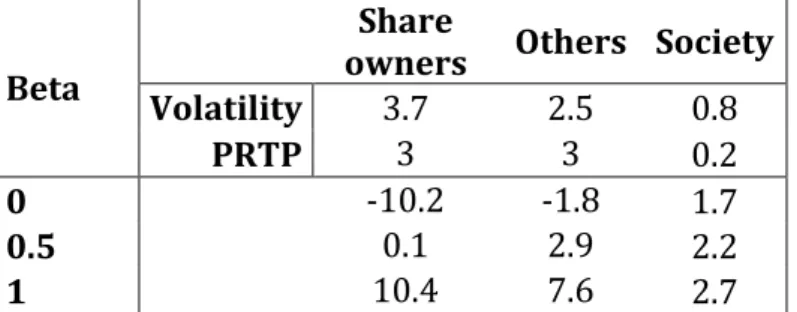
However, even if intra-generational equality is ignored and if individuals are purely self-interested and rational, there are two compelling arguments for a lower social discount rate (for risky assets) than the individual one. The first is that the hazard risk is much higher for individuals separately than for society entirely, implying a larger pure rate of time preference for individuals. More importantly, the second is due to consumption risk sharing. Although Arrow and Lind (1970) were not right in that risk pooling between individuals erases structural risk from social discounting, risk pooling clearly reduces the influence, illustrated in Table 2. From my perspective this is the most basic argument for a prescriptive rather than descriptive approach in a small open economy. However, it is odd that the prescriptive focus has been almost exclusively on the STP, while the prescriptive SOC method has been more or less ignored, 21.
Table 2: Risk-adjusted time preferences for individuals versus society, using the combination of eq. (4). and eqs. (3) and (6) with η=1.5 and μ =1.5.
Beta
Share
owners Others Society
Volatility 3.7 2.5 0.8
PRTP 3 3 0.2
0 -10.2 -1.8 1.7
0.5 0.1 2.9 2.2
1 10.4 7.6 2.7
Further, the descriptive approach may be harder to estimate in practice, since it is hard to anticipate how agents will act, that is, it is hard to estimate the correct mix of ROI, FB and CRI. Further, the standard version of the descriptive approach, seem to be customized for a large economy such as the US, possibly making it less relevant for a small, open economy. The geographic area of optimization constitutes an extra dimension to the problem. It is not completely straight forward if global or national optimization is the aim. 22
The prescriptive approach on the other hand depends on the assumption on rational governance (social planner). Here also the problem remains of deciding on which of SOC and the (displacement adjusted) STP to be chosen. In theory, under perfectly rational governance, they should be equal, but what if they are not? Then there are at least two reason for this. The simplest one is that the discrepancy is due to measurement errors. Then if one possibly assumes that the
21 This could possibly be due confusion between prescriptive/STP methods, due to a sloppy and
unsuitable terminology tradition.
22 The method considers the real return of investment (before corporate tax). If Swedish citizens
diverse their asset portfolios in an optimal way, only a small fraction of their investments will be in Swedish companies (since Sweden is a small open economy), making the benefits of corporate taxes from such investment a minor issue. Moreover, with global market pricing of Swedish companies, it is likely that foreign investors would fill in such capital gap (which is a relevant objection of the method also for a large economy, if the objective is to maximize nationally only). It therefor seems as the descriptive SOC method is relevant only if objective is to 1) optimize globally, 2) employ Kaldor-Hicks criterion, 3) not allow public investments in global capital market.
17
errors of SOC and STP approaches are of similar order, an unbiased estimator of the SDR is mean(STP, SOC).
Another interpretation is that government is not completely rational or lack information, which constitutes an alternative hypothesis of what might generate the discrepancy between STP and SOC. E.g. if it turns out that the risk-adjusted return is larger on global capital market than the STP suggests, then it would be rational to increase centralized investment in the global capital market. This action would increase the prospects of consumption growth, pushing up the STP value towards the SOC value. If on the other hand the SOC value is smaller STP value, then this implies that it is not possible to achieve a return high enough to motivate investments from a preference perspective, and it would be rational to decrease public investments in global capital markets (given that such investments exist). But there may exist restrictions, which prevent the government from changing the level of investment in global capital markets. If the budget for such investments is fixed, then this return is not relevant, but STP seems as the relevant candidate for the SDR. If one possibly considers all these three possibilities as likely, then a feasible estimator of the prescriptive SDR is:
SDR� = mean �mean(SOC, STP) ; SOC; STP� = mean(SOC, STP) (8) In Appendix B, I elaborate further on these thoughts. To conclude, if one assumes that government is maximizing national welfare, the SDR for various feasible assumptions is constrained between the national STP and the global SOC23.
3.2 The normal distributed growth assumption
Even though the CAPM has proven poor from descriptive point, it may be useful from a normative point. A remaining problem with CAPM is that it is based on the assumption of thin-tail (normal) uncertainty of economic development, when in reality uncertainty may very well be fat-tail. From this perspective, the CAPM structure may underestimate uncertainty, but can been seen as a first step in the effort to fully account for uncertainty about future states of the world.
Gollier (2014) shows that if growth follows a Brownian motion, the discount structure is flat. Weitzman (2007) makes a compelling argument against the Brownian motion, but then the question of limitations in estimation remains. For the special case of lognormally distributed future consumption with autocorrelated growth, the social discount rate is declining only for the case 𝛽𝛽 < 𝜂𝜂
2 (Gollier, 2014), which does not seem to hold for Swedish infrastructure investments (𝛽𝛽 ≥ 0.82 in Hultkrantz et al. (2014) and 𝜂𝜂 = 1.5 in Groom & Maddison 2018). To summarize, given the current state of knowledge, discount rates for Swedish infrastructure investments could have a decreasing, flat or increasing terms structure, dependent on various plausible assumptions on the
23 An additional minor problem with the SOC methods that it is not explicit what the implicit
growth expectations are (by the market), so it is not clear if these expectations are consistent with the with forecast used for CBA.
18
structure on macroeconomic uncertainty. For this reason, I will use a flat term structure as a base case.
However, there may still be some pragmatic possibilities to incorporate some of the structural uncertainty. The idea is to simply use the flat CCAPM formulas, but to assume that the normal distribution estimation will underestimate the growth standard deviation, due to structural uncertainty (in line with Weitzman’s 2007 reasoning). However, when using this approach, the question next in line is “how much is the standard deviation underestimated?”, which is a rather subjective question. A starting point could be to perform sensitivity analysis with for example a doubled standard deviation. Another possibility is to look at the variance of longer time periods (e.g. 10 or 30 y). A third option is to use Weitzman’s revealed estimates of structural uncertainty from stock markets.
3.3 Option value
It seems as the discussion about the discount rate as a decision guiding tool, until now has been focused quantity of realization of projects (how much CO2 mitigation is optimal, how much resources should be spent on road investments, should a specific project be realized or not), and to a lesser extent on ranking of projects. Timing of investment here seems like a more or less overlooked issue. Real option values increase in importance with the prospect of better information in the future. Real option value in a public setting differs from private ones, in that private option values are linked to game theory (strategic investments, market shares), which may imply to invest more than when only considering traditional NPV, while this is not the case for real option value in a public setting. For public investments, I argue, real option value is mainly about depleting an option as an investment is realized, and hence, less investments should be executed than the ones that pass a cost-benefit test. Ultimately, option value analysis should be performed in a thorough manner, using a method similar to Krüger (2012b)24, or even better so, a method that also accounts for learning. However, such a method may be too costly for small project. An alternative could be to account for option value to some extent through the discount rate, and hence guide the timing decision. In line with de Rus (2011), I argue that if project specific risk is ignored in traditional discounting, there is an additional real option value in postponing investment decision one year, until some uncertainty may have materialized. For projects close to break-even in terms of net benefit cost ratios, the costs of postponing a project one year is probably small, while there are gains in terms of the possibility to exclude bad investments. From this perspective I argue that an extra (positive) term should be added to discount rates for discrete investments. However, since I have not been able to find any literature on the value of information, the size on such term is much unclear. However, Krüger (2012b) estimates the pure value of waiting for two cases, and these could be recalculated to discount rate components.
19
3.4 CO2 emissions
A decision to physically alter the transport infrastructure will affect yearly emissions for a long time period; typically, during the life-time of the project. How should one discount emissions that accrue 15 or 30 years from now, in the light of deep uncertainty about the true cost about these emissions? One might think that beta of emissions is the same as of damage estimation. I argue that it is not, since such approach ignores relevant alternative options. It is possible that 10 years from now the understanding of these damages has been much improved25, and that we then value emission much different from now. What is the beta of such CO2 emissions? If we then find out that SCC will be close to zero, previous investments to reduce CO2 will be worthless. If on the other hand it turns out that SCC is much higher, returns to such investment will be greater, but if an investment hasn’t been realized yet, it will probably not be too late to do so. Hence, there is a real option value to take in to account. In the same time, a possibly higher future SCC estimates will decrease the return on investments that increase CO2 emissions, but there will likely exist other means to reduce CO2 emissions than to decrease travel demand, so project risk is not completely symmetric in this sense. Appendix C gives some sketchy structure to these arguments. A conclusion is that while waiting for more research on the matter, it does not seem unreasonable to use the same beta for CO2 emission reductions as for other transport related benefits.
4 METHOD
In the present study, I estimate SDR for Swedish infrastructure investments based on theory and parameter values from section 2. In line with the reasoning in section 3, focus is on the prescriptive approach (both STP and SOC versions), using eqs. 3, 4 and 6. To estimate the opportunity cost by alternative use in public sector seems a too demanding task and will be out of the scope of the present study. Instead estimates of returns on financial market (as in Hultkrantz et al. 2014) will be used as opportunity cost. In line with the reasoning in section 3, the mean of STP and SOC approaches (eq. (8)) will be considered the best estimate. The main analysis includes a social PRTP of 0.2%/y, growth rate of 1.5%/y (to be consistent with the Swedish national guidelines 26). For the best estimate, a modest (ad-hoc) increase in the standard deviation of growth, compared to estimates from a normal distribution is applied, along with a modest time premium. Sensitivity analyses on parameter values are carried out for each approach respectively. In addition, a much sketchy attempt to a descriptive approach is presented in Appendix B. Results are presented next, in section 5.
25 Generalized climate sensitivity (including all feedback loops) is highly uncertain, and estimates
will probably be more accurate the longer time-series of emissions and temperature are available. There is also a strong and ongoing development in theories of handling such risk in damage estimation. These two factors to a substantial extent explain the fundamental uncertainty in SCC estimation (see e.g. Hope, 2006, Hope, C., 2008a, Anthoff et al. 2009), and hence it is plausible to believe that SCC will be more accurate and possibly less uncertain in 10 years from now.
20
5 RESULTS
Table 2 present SDR estimates for a stationary normal distribution of growth, with no timing premium. Table 3 includes sensitivity analyses with respect of the STP approach. Table 4 provide time premium estimates and Table 5 present best estimates. In Table 6, the NPV implications are tested for a real case, investment is HSR in Sweden.
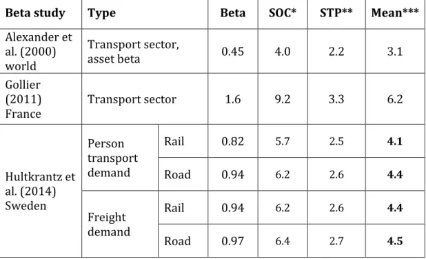
Table 2: SDR estimates (%) with SOC, STP and mix methods, eq. (4). SOC 𝑟𝑟𝑓𝑓 = 2% and 𝜋𝜋 = 4.5% are from Hultkranz et al. (2014) (same as in NOU 2012:16). STP 𝑟𝑟𝑓𝑓 and 𝜋𝜋 are based on eqs. (3) and (6) respectively, using 𝛿𝛿 = 0.2, 𝜂𝜂=1.5, 𝜇𝜇 = 1.5 and 𝜎𝜎 = 0.8. Bold figures denote SDR best estimates.
Beta study Type Beta SOC* STP** Mean***
Alexander et al. (2000) world Transport sector, asset beta 0.45 4.0 2.2 3.1 Gollier (2011)
France Transport sector 1.6 9.2 3.3 6.2
Hultkrantz et al. (2014) Sweden Person transport demand Rail 0.82 5.7 2.5 4.1 Road 0.94 6.2 2.6 4.4 Freight demand Rail 0.94 6.2 2.6 4.4 Road 0.97 6.4 2.7 4.5
*SOC is based on the assumption that an alternative to the project is that government invest in global capital market.
**STP is based on the assumption that the government budget on alternative investments is fixed.
***Mean is the mean of these two, coincides with the formula:
SDR� = mean(SOC, STP) (eq. (8)) and considered the best estimate (see section 3.1).
Table 3: Sensitivity of STP method (beta 0.94 from Hultkrantz et al., 2014). Bold figure (2.6%) denote main analysis (in Table 2).
EMUC Volatility
0.8 1.6 3.2
1 2.0% 2.8% 6.2%
21
Analogous sensitivity analyses for various beta values are found in Appendix D. Table 4: The value of delaying investment, based on Krüger (2012b)
Case increase NPV (years) Delay Increase per y. delay
3-lanes +11% 15 +0.7%
4-lanes +137% 20 +4.4%
Table 5: Best SDR estimates (%), using 𝜎𝜎 = 1 and a timing premium of 0.7%.
Type Mode NPV* NPV + timing
Person
transport Rail Road 4.1 4.5 4.8 5.2 Freight Rail 4.5 5.2
Road 4.6 5.3
Mean 4.4 5.1
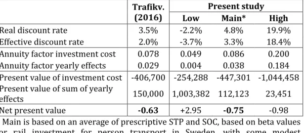
*If objective is only to calculate the absolute net present value of a projects Table 6: Sensitivity HSR proposal in Sweden (from Trafikverket, 2016b). Discounting and traffic start year is 2020 (building time 15 years, effect calculation period 60 y).
Trafikv. (2016) Low Present study Main* High
Real discount rate 3.5% -2.2% 4.8% 19.9%
Effective discount rate 2.0% -3.7% 3.3% 18.4%
Annuity factor investment cost 0.078 0.049 0.086 0.200 Annuity factor yearly effects 0.029 0.004 0.038 0.184 Present value of investment cost -406,700 -254,288 -447,301 -1,044,458 Present value of sum of yearly
effects 150,000 1,003,382 112,123 23,451
Net present value -0.63 +2.95 -0.75 -0.98
* Main is based on an average of prescriptive STP and SOC, based on beta values for rail investment for person transport in Sweden, with some modest adjustment for macroeconomic tail events and optimal timing.
The highest and lowest estimates are both based on the STP method. They further assume very high volatility of 3.2 (four time the empirically estimated one) and a main case EMUC value of 1.5. Both are based on stock market betas (e.g. asset betas) outside of Sweden, so the relevance is not straight forward. The low estimate is based on beta = 0.45 from Alexander et al. (2000), and stationary normally distributed macroeconomic growth (volatility 0.8), and no timing premium, see Table Appendix D. Since this estimate is considerably lower than the corresponding SOC estimate (Table 2), it requires the additional assumption
22
that government investment in global capital market is not a relevant option. The High estimate is based on beta = 1.6 from Gollier (2011), combined with intertemporal EMUC values of 1.5 and highly uncertain macroeconomic growth (volatility 3.2). This gives a STP of 15.5%, see Appendix D. A large timing premium of 4.4% from Table 5 has been added.
6 DISCUSSION
Within the STP method, estimates vary greatly, and here the most important source of uncertainty is the sector beta (see Appendix D). This is rather natural, considering that this is a new area of research, with only a few relevant estimates available. However, this source of uncertainty is present also for SOC approach. But when combined with the other sources of uncertainty, in particular the volatility uncertainty, then the STP approach becomes highly sensitive, possibly to the extent that it undermines the approach as such.
Current estimates of SDR is Sweden is based on a traditional STP method. The new STP method, including uncertainty about growth yield a much similar main estimate as the official figure, although parameter values of PRTP and EMUC has been updated (but in different directions). However, it is not clear that the STP method is more appropriate than the social planner version of SOC method, which yield considerably higher main estimates.
The projected 1.5 growth rate is somewhat low compared with current records. If future growth will be closer to 2%, the real SDR in the present study is somewhat underestimated (about 0.5%). However, best estimates of effective SDR for VSL and VTT (including relative price increases) will not be much affected (see Appendix E), since also the relative prices of benefits should be increased. The present study sketches the method of how to consistently estimate the SDR for transport infrastructure investments in a small open economy, i.e. Sweden, based on current state of art. However, parts of that sketch are still incomplete, implying a need to elaborate on these issues in future research. The maybe most neglected issue is how to incorporate option value into the SDR, and there should be much room for theoretical advancements in this area.
Estimation of relevant beta values are generally in an early stage of research, including the understanding of the climate beta27. Empirical estimation of investment cost beta could be worthwhile. Estimation of the complete beta for benefits of investments, including relative price changes of time and life would be welcome. Estimation of beta values for air- and maritime transport investments is a natural expansion. There is also a potential of improvement through further disaggregation of beta estimates in general. For example, by various categories of projects, or by VSL and VTT. A theory of how to consistently translate the income
27 Research needs includes a complete theory of emissions beta as well as improvement of risk
23
elasticity of VSL into a VSL beta could provide a way forward. Finally, a theory of the social valuation of real estate returns along with empirics is needed.
7 CONCLUSIONS
This paper outlines the theoretical structure for determining the appropriate SDR for infrastructure investments in a small open economy with social preferences for smoothed distribution of consumption, e.g. Sweden. Most of these theories are valid also in the more general setting of public investments in a small open economy. However, the empirics for such calculation are only partly understood (both in qualitative (underlying assumptions) and quantitative terms), meaning the estimates in the present paper are
preliminary. The best estimate of the present study SDR for land transport infrastructure investment in Sweden is about 4.4%, if CBA is only to calculate expected absolute net present values of investments. If optimal timing of investment is also considered, then the SDR best estimate is about 5.1%.
Disaggregated on freight vs. person transport, and on road vs. rail transport the last type range from 4.8% to 5.2% depending on type of investment.
Considering the large degree of uncertainty involved, the need for disaggregated SDR does not seem urgent in practice.
These figures include some consideration of macroeconomic tail-events, not captured by the normal distribution and adjustment for optimal timing of investments, pushing up the estimates somewhat compared to if such adjustments are not made. However, since the empirical evidence on these adjustments is thin, a conservative approach has been chosen, only making minor adjustments. This means that the SDR may still be underestimated. There is a great need to elaborate further on these two issues in the future, as well as to further discuss which are the most reasonable underlying assumptions determining the choice of STP vs. SOC approaches.
There is also a risk that the SDR is underestimated due to the fact that relative price increases of time and life was not included in the beta-estimates. In addition, an update of the relative price projections in the Swedish guidelines (ASEK) would be welcome, especially when it comes to carbon dioxide emissions and for VSL. VSL seems to be growing considerably slower than income (for rich countries), with an income elasticity of about 0.55 (Masterman and Viscusi, 2018). For carbon dioxide, it is recommended to adjust the projected yearly relative price increase, from 1.5% to 2.7 % (based on Asplund, 2018).
If implementing this “newish” approach of including macroeconomic risk in the discount rate, such risk should not be double counted. I.e., these discount rates should not be combined with sensitivity analysis of general economic growth.
24
This study has been financed by The Swedish Transport Agency. I thank Professor Lars Hultkranz, Örebro university and Docent Svante Mandell, the National Institute of Economic Research (Sweden), for valuable comments.
25
REFERENCES
Alexander, I., Antonio Estache, A. , Oliveri, A. (2000). "A few things transport regulators should know about risk and the cost of capital", Utilities Policy, 9, 1–13
Andersson, H., Hultkrantz, L., Lindberg, G., & Nilsson, J. (2018). Economic Analysis and Investment Priorities in Sweden’s Transport Sector.
Journal of Benefit-Cost Analysis, 9(1), 120-146. doi:10.1017/bca.2018.3
Anthoff, D., Tol, R. S. J. & Yohe, G. W. (2009). “Risk aversion, time preference, and the social cost of carbon”, Environmental Research Letters, vol. 4
Arrow, K. J. , Lind, R. C. (1970). "Uncertainty and the Evaluation of Public Investment Decisions," Amer. Econ. Rev., 60, 364-78.
Arrow, K. J., et al. (2013). How Should Benefits and Costs Be Discounted in an
Intergenerational Context?, Economics Department Working Paper
Series No. 56-2013, University of Sussex
Asplund, D. (2017). "Household Production and the Elasticity of Marginal Utility of Consumption", The B.E. Journal of Economic Analysis & Policy, DOI: 10.1515/bejeap-2016-0265
Asplund, D. (2018). "The temporal aspects of the social cost of greenhouse gases", ECONOMICS and POLICY of ENERGY and the ENVIRONMENT, 2017:3, Pp. 25-39, DOI: 10.3280/EFE2017-003002,
https://www.francoangeli.it/riviste/Scheda_Rivista.aspx?IDArticolo=6 2150&Tipo=Articolo%20PDF&idRivista=10&lingua=en
Atkinson, G., Dietz S., Helgeson, J., Hepburn, C., Sælen, H. (2009). "Siblings, not triplets: social preferences for risk, inequality and time in discounting climate change", Economics, Vol. 3, 2009-26, http://www.economics-ejournal.org/economics/journalarticles/2009-26
Attanasio, O., P., Banks, J., Tanner, S. (2002). "Asset Holding and Consumption Volatility", Journal of Political Economy, vol. 110, no. 4
Baum, S. (2009). “Description, prescription and the choice of discount rates”,
Ecological Economics, vol. 69, pp. 197–205
Baumstark, L., Gollier, C. (2014). "The relevance and the limits of the Arrow-Lind Theorem", Journal of Natural Resources Policy Research, 6:1, 45-49, DOI: 10.1080/19390459.2013.861160
Barro, R., J. (2006). Rare disasters and asset markets in the twentieth century, The Quarterly Journal of Economics, Vol. 121, Iss. 3, Pp 823–866
Boadway, R., (2006). Principles of Cost-Benefit Analysis. Public Policy Review, 2 (1).
26
Bradford, D. F. (1975). "Constraints on government investment opportunities and the choice of discount rate". American Economic Review 65(5), 887– 899
Börjesson, M. Fosgerau, M., Algers, S. (2012). "On the income elasticity of the value of travel time", Transportation Research Part A: Policy and
Practice, Vol. 46, Iss. 2, pp 368 - 377
https://doi.org/10.1016/j.tra.2011.10.007
Cropper, M., L., Freeman, M., C., Groom, B., Pizer, W. A., (2014). "Declining Discount Rates", American Economic Review: Papers & Proceedings, vol. 104(5), pp. 538–543. http://dx.doi.org/10.1257/aer.104.5.538
Dasgupta, P., (2008). “Discounting Climate Change”, Journal of Risk and
Uncertainty, vol. 37, pp. 141-169.
Dasgupta, Partha and G. M. Heal. 1979. Economic Theory and Exhaustible
Resources. Cambridge: Cambridge University Press
Dietz, S., Gollier, C., Kessler, L, (2018). "The climate beta", Journal of
Environmental Economics and Management, 87(2018)258–274
De Rus, G. (2011). "The BCA of HSR: Should the Government Invest in High Speed Rail Infrastructure?," Journal of Benefit-Cost Analysis: Vol. 2: Iss. 1, Article 2. DOI: 10.2202/2152-2812.105
Drupp, M.A., Freeman, M.C., Groom, B., Nesje, F. (2018), "Discounting Disentangled." American Economic Journal: Economic Policy, 10 (4):109-34. DOI: 10.1257/pol.20160240
Drupp, M. A., Hänsel, M. C. (2018). Relative Prices and Climate Policy: How the
Scarcity of Non-Market Goods Drives Policy Evaluation, Economics
Working Paper, No. 2018-01, issn 2193-2476
Edlund, K., Gunnarson, G., Johansson, M., Mård, C., Stjerkvist, L., Svedahl, R. (2016). "Kalkylen talar för höghastighetståg", Dagens samhälle, 2016-11-15. https://www.dagenssamhalle.se/debatt/kalkylen-talar-foer-hoeghastighetstag-29349?story=2381
Eliasson, J., Börjesson, M., Odeck, J., Welde, M. (2015). "Does Benefit–Cost Efficiency Influence Transport Investment Decisions?", Journal of
Transport Economics and Policy, Volume 49, Part 3, pp. 377–396
Engström Stensson et al., (2014). En guide till Europas utsläppshandel, Fores studie 2014, ISBN: 978-91-87379-20-8
Emmerling, J., Groom, B., Wettingfeld, T. (2017). “Discounting and the
representative median agent”, Economics Letters, Vol. 161, Pp 78-81, ISSN 0165-1765, https://doi.org/10.1016/j.econlet.2017.09.031.