Waveform clustering

(1)

V¨

aster˚

as, Sweden

Thesis for the Degree of Master of Science in Engineering - Robotics

30.0 credits

-GROUPING SIMILAR POWER

SYSTEM EVENTS

Ther´ese Eriksson

ten09003@student.mdh.se

Mohamed Mahmoud Abdelnaeim

mmm14001@student.mdh.se

(2)

Supervisor at the company: Shiva Sander-Tavallaey

Supervisor at the company: Tord Bengtsson

Supervisor at MDH:

Elaine ˚

Astrand

M¨

alardalen University, V¨

aster˚

as, Sweden

Supervisor at MDH:

Joaqu´ın Ballesteros

M¨

alardalen University, V¨

aster˚

as, Sweden

Examiner:

Ning Xiong

M¨

alardalen University, V¨

aster˚

as, Sweden

(3)

Abstract

Over the last decade, data has become a highly valuable resource. Electrical power grids deal with large quantities of data, and continuously collect this for analytical purposes. Anomalies that occur within this data is important to identify since they could cause nonoptimal performance within the substations, or in worse cases damage to the substations themselves. However, large datasets in the order of millions are hard or even impossible to gain a reasonable overview of the data manually. When collecting data from electrical power grids, predefined triggering criteria are often used to indicate that an event has occurred within the specific system. This makes it difficult to search for events that are unknown to the operator of the deployed acquisition system. Clustering, an un-supervised machine learning method, can be utilised for fault prediction within systems generating large amounts of multivariate time-series data without labels and can group data more efficiently and without the bias of a human operator. A large number of clustering techniques exist, as well as methods for extracting information from the data itself, and identification of these was of utmost importance. This thesis work presents a study of the methods involved in the creation of such a clustering system which is suitable for the specific type of data. The objective of the study was to identify methods that enables finding the underlying structures of the data and cluster the data based on these. The signals were split into multiple frequency sub-bands and from these features could be extracted and evaluated. Using suitable combinations of features the data was clustered with two different clustering algorithms, CLARA and CLARANS, and evaluated with established quality analysis methods. The results indicate that CLARA performed overall best on all the tested feature sets. The formed clusters hold valuable information such as indications of unknown events within the system, and if similar events are clustered together this can assist a human operator further to investigate the importance of the clusters themselves. A further conclusion from the results is that research into the use of more optimised clustering algorithms is necessary so that expansion into larger datasets can be considered.

Keywords— Unsupervised learning; clustering; multivariate time-series data; discrete wavelet transform; power transformer

(4)

Abbreviations

AC Alternating Current

ADMO Absolut Distance between Medoid and Object AGNES Agglomerative Nesting

AI Artificial Intelligence

BPNN Back-Propagation Neural Network CFDP Clustering Finding Density Peaks CLARA Clustering for LARge Application

CLARANS Clustering for Large Applications based on RANdomized Search Db Daubechies

DBSCAN Density-Based Spatial Clustering of Applications with Noise DFT Discrete Fourier Transform

DGA Dissolved Gas Analysis DIANA DIvisive ANAlysis DOG Difference-Of-Gaussian DTW Dynamic Time Warping DWT Discrete Wavelet Transform FCM Fuzzy C-Means

FM Fowlkes-Mallows index FT Fourier Transform HV High Voltage

HTM Hierarchical Temporal Memory HP High Pass

KPCM Possibilistic C-Means algorithm LP Low Pass

LV Low Voltage

MAVS Mean Absolute Value slope ML Machine Learning

MPV Maxium Peak Value NCR Normalised Class size Rand

NIPALS Non-linear Iterative Partials Least Square PAM Partition Around Medoids

PCA Principal Component Analysis PCM Possibilistic C-Means

PGDCS Power Grid Dispatch and Control System QT Quality Threshold

RMS Root Mean Square SAE Sparse AutoEncoder SD Standard Deviation

SDR Sparse Distributed Representation SSE Sum of Squared Error

(5)

3.7.3 Model-based clustering . . . 16 3.7.4 Density-based clustering . . . 16 3.8 Similarity measurement . . . 17 3.8.1 Lock-step measurements . . . 17 3.8.2 Elastic measurements . . . 18 3.9 Quality analysis . . . 19 3.9.1 External criteria . . . 19 3.9.2 Internal criteria . . . 19 3.9.3 Relative criteria . . . 22 4 Related work 23 4.1 Summary . . . 25

5 Ethical and societal considerations 26 6 Methods and implementation 27 6.1 Methodology . . . 28

6.2 Process flow setups . . . 28

6.2.1 Analysis of the ABB dataset . . . 28

6.2.2 Feature processing . . . 28

6.2.3 Clustering algorithms . . . 28

6.2.4 Distance measurements . . . 29

6.2.5 Clustering evaluation methods . . . 29

6.2.6 Limitations of test cases . . . 29

6.3 Data acquisition and handling . . . 30

6.3.1 Segmentation of data . . . 30

6.4 Data transformation . . . 30

6.5 Initial test setup . . . 31

6.6 Frequency extraction - Discrete wavelet transform . . . 32

6.7 Feature selection - Laplacian score . . . 32

(6)

6.9 Feature reduction - Principal component analysis . . . 33 6.10 Outlier handling . . . 33 6.11 Clustering . . . 33 6.11.1 CLARANS . . . 33 6.11.2 CLARA . . . 36 6.12 Similarity measurement . . . 38 6.13 Quality analysis . . . 38 7 Results 39 7.1 Initial test phase . . . 39

7.1.1 PCA . . . 39

7.1.2 Clustering . . . 39

7.2 Second test phase . . . 40

7.2.1 Feature evaluation and selection . . . 40

7.2.2 PCA . . . 41

7.2.3 Decide the number of clusters . . . 42

7.3 Final test phase . . . 48

7.3.1 Test with larger dataset . . . 49

7.3.2 Test with feature reduction . . . 51

8 Discussion 54 9 Conclusions and future work 56 9.1 Future work . . . 57

10 Acknowledgements 58

(7)

1 Introduction

The use of acquisition systems is increasing drastically since data is a highly valuable resource for analytical purposes. ABB Corporate Research has established multiple acquisition systems that are continuously reading voltage and current data at a number of transformers on the electrical grid. The monitored waveforms from the power systems are three-phase sinusoidals with a frequency of 50 Hz. However, the acquisition systems are only storing the data when a predefined trigger criterion is fulfilled in order to limit the amount of collected data. This is referred to as an event within the transformer system. There are scanning tools available to find known events within the collected data, but the predefined criteria make it difficult to search for events occurring that are unknown to the operator of the tool. The reason for this is that the trigger catches large amounts of events of both known and unknown type, and the unknown types need to be manually searched for in order to be identified. It is important to find these unknown events because they could cause nonoptimal performance within the substations, or in worse cases damage to the substations themselves. Since transformers are some of the most costly parts in a power system, being able to perform preventative maintenance in place of corrective maintenance could cut down not only costs but also time and safety hazards since they typically are not constructed until commissioned [1]. ABB is currently online monitoring power system data through the tool Transformer Explorer, which stores current and voltage information while the transformer is in service. From this information, parameters relating to the state of the transformers turn ratio, short-circuit impedance, and power loss is obtained. However, the use of this application is handled manually which could lead to human errors. In order to prevent disruptions caused by corrective maintenance, as well as gain a deeper understanding of the system behaviour in general, an automated tool that can catch occurring events within the system is necessary. Datta et al. [2] discuss the advantages of using unsupervised methods such as clustering for fault prediction within systems generating large amounts of data. As such, to analyse the large amounts of waveform data, feature extraction can be performed on the signals and then used in creating groups of events, also known as clusters. Clustering is an artificial intelligence (AI) technique in the category of unsupervised learning and has several different applications such as robotics, data mining, and computer vision. Russell and Norvig [3] describes unsupervised clustering as ”the problem of discerning multiple categories in a collection of objects”. The objects for transformer signal analysis is, in this case, the events of different types within the data, and the categories are the types themselves. In order to find these events and discern them from the uneventful data logs, an automatic sorting functionality to separate these would be beneficial. With the help of this functionality, only a few events within each cluster needs to be inspected manually, and if deemed of no importance the cluster can be discarded. If the events within a formed cluster are something new and/or of interest the entire cluster can be further analysed.

1.1 Goal of thesis

The objective of the study is to research methods that enable finding patterns unknown to the transformer model currently in use by ABB by analysing the current and voltage signals [4]. A deeper understanding of the large amount of available data is one of the expected outcomes. In order to group data with similar properties, an analysis of clustering methods that have been eval-uated for the purpose of grouping data with similar properties will be presented, and a similarity measurement of the clustered data will be performed. These clustering methods should be imple-mented as well as adjusted to handle large amounts of waveform data. The impleimple-mented system should be able to detect and cluster types of events unknown to the current system in use. A summary of the benefits of the proposed automated system compared with a manual classification will be done. The work falls into two categories; signal processing and feature extraction, and clustering of data and quality analysis of the clustering.

1.2 Outline of thesis

The problem formulation with associated research questions is stated in section 2. General informa-tion regarding transformer theory and applicainforma-tions, signal processing basics, as well as clustering

(8)

methods can be seen in section 3. Section 4 holds an overview of the related works with the state of the art in regards to waveform analysis and clustering in power systems as well as the handling of time-series data. The ethical and societal considerations relevant to the thesis are described in section 5. Section 6 describes the methodology employed within the thesis work as well as the information regarding the implementation of it, while section 7 holds the results. Section 8 holds a discussion about the achieved results of the thesis in regards to the stated goals, and lastly, section 9 holds the final thoughts on the impact of this work as well as a presentation of future work in the area.

(9)

2 Problem Formulation

The collected data which is stored in the form of an event database makes it currently unfeasible to gain a broad overview of the entire content. A more structured database with identified clusters of event data would be beneficial which could enable new events from an online stream to be classified into the cluster with the highest similarity to it. Not all events would be of interest, and this information can be further used to prevent the collection of irrelevant data.

2.1 Research questions

1. Which types of clustering methods can be used for grouping events occurring in power systems?

There exists a large number of clustering methods and an extensive literature review is necessary in order to identify suitable techniques.

2. How can the suggested clustering method be integrated and automated?

Investigation of the possibility to incorporate the suggested clustering method with existing trigger-based acquisition system that are continuously monitoring the voltage and current of transformers.

3. Which discriminating features of the event signals are important for the cluster-ing?

Features that contain descriptive information that can identify the different events needs to be recognised and evaluated.

4. What is the quality of the clustering?

The quality of the clustering needs to be investigated for similarity, where a high similarity indicates similar types of events.

2.2 Limitations

Some limitations exist that could affect the execution and results of the proposed research. These are mainly concerned with the involved data and the handling of this, as well as the confidentiality surrounding it. One limitation set by ABB Corporate Research is the available data set that will be analysed. At the time of writing, many years of data have been logged from the transformers in the substations mentioned. However, an analysis will only be performed on a selected subset of this data to make the work possible within the time frame. Another important aspect is that the data is the property of ABB Corporate Research, and as such, could be sensitive information and should be protected from exposure outside of internal settings. Sensitive data has the possibility to be anonymised within the final report, with the specific details placed within an appendix that is only available to ABB Corporate Research.

(10)

3 Background

As the first phase of this thesis work, a comprehensive literature study was conducted regarding different areas related to this specific research topic. Described in the following section is the background information necessary in order to place the thesis work within the proper context. This included the basics of transformer characteristics such as important structural design, typical applications, as well as problems that can occur within transformers. Following this is information regarding online and offline methods for monitoring of transformer systems. Since the typical signals available in power system transformers consists of waveform signals, another crucial area is the analysis of time-series and waveform data handling, and how to process this type of data. An overview of the common methods to extract and handle waveform signal and time-series data as well as some basic concepts regarding signal processing included. A section detailing the different methods that can be used to measure distance, or similarity, between time-series data follows and Lastly is an examination of different clustering methods, necessary steps involved, and the motivation for using different approaches for different applications.

3.1 Transformer theory and application

A transformer is an electrical component usually used to transform an incoming alternating current (AC) voltage level to a different level, either by stepping the voltage up or down; this is done by a mechanical operation known as tap change where the number of turns of a winding is changed [5]. This is crucial for our modern day electricity transmission line set-up. Transferring electricity over long distances creates a power loss depending on transmission line resistance as discussed by So and Arseneau [6]. This loss can be limited when transferring electricity by increasing the voltage level and lowering the current, but before the power reaches its destination such as a typical household, the voltage level needs to be lowered; this is typically done with transformers. A simple transformer usually consists of two coils constructed out of metal wire, commonly referred to as the primary and secondary winding. The primary winding is supplied with a voltage, and this winding then produces a magnetic field; the magnetic flux marked as a dotted red line flows through the core as a consequence of this as seen in Figure 1. The magnetic field induces a voltage output that is dependent on the turn ratio of the primary and secondary coil. A single transformer is usually not used, but instead three; this is more commonly implemented since three-phase electricity is produced from power station generators. In a paper presented by Suppitaksakul et al. [7], the process of determining the power and size of three-phase induction generators is discussed. The mathematical model of the proposed induction generator is tested and compared with both simulated and experimental results; it is concluded that the proposed mathematical model can be used for selecting generator size.

Figure 1. Simple transformer where two windings are wrapped around a magnetic core. The dotted red line is the magnetic flux running through the magnetised core.

Typical applications for transformers are mainly in industrial settings such as power systems, communications, automotive, and steel manufacturing. The transformers usually employed for power systems fall into two categories; power transformers and distribution transformers [8]. Power transformers, which are large in size and transform high levels of voltage, is the type which is

(11)

manufactured by ABB in order to transmit generated power between stations in the electrical grid. Distribution transformers are used for lowering the voltage to a level that fits the consumer. Failure origination for faults that occur in power system transformers falls into mainly four categories: windings, tap changers, bushings, and lead exits. The distribution of these can be seen in Figure 2, where a fifth category ’Other’ can also be observed. This category represents fault originations such as core circuits, magnetic circuits, and insulation. Winding faults, representing the largest fault category, are affected by mechanical forces proportional to the current squared [8]. This can lead to buckling in the winding itself, altering the short-circuit impedance of the system. Faults originating in the tap changer are usually related to mechanical aspects since the component moves during operation of the transformer.

Figure 2. Pie chart of failure origination distribution as seen in Survey by Tenbohlen and Jagers [9].

3.2 Offline and online monitoring

The evaluation of transformers in test laboratories can be done by analysing the impulse response of a specified transfer function. The transformers’ transfer function can be applied when monitoring the transformers while functioning out in the field as well. In a study by Leibfried and Feser [10] the application of transfer function for offline and online monitoring is discussed. When monitoring offline, the transformer is disconnected from the electrical grid thereafter switched on and off, and the acquisition system reads the voltage and current through a digital measuring system. Online monitoring is similarly done, but instead, the measurements are performed when the transformer is active and functioning. In the previously discussed study, two methods are mentioned which are commonly integrated into transformers offline/online monitoring system and are said to be important monitoring techniques. First is the gas-in-oil analysis; this method is discussed in a paper written by Chatterjee et al. [11] where the information on how to measure dissolved gases and temperature from the transformer oil is discussed. With correct readings, it is possible to predict potential or already occurring faults. The second method is the partial discharge measurement; a paper written by Jacob and McDermid [12] discusses the importance of this method regarding acceptance test of transformers. The data collected by ABB, intended for analysing and clustering, is collected from several active transformers via online monitoring without considering gas-in-oil and partial discharge analysis.

(12)

3.3 Transformer data

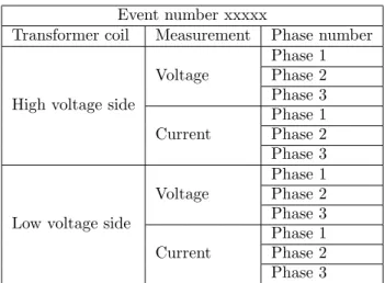
There are different measurements that can be collected from transformers in service. The ABB data consists of voltage and current signals which are measured from different three-phase transformers. That means that the acquisition systems retrieves a voltage and current signal from each phase, in both primary and secondary windings. This gives three current signals and three voltage signals from the primary winding, and similarly for the secondary, giving a total of twelve signals. ABB is currently running the signals through the tool Transformer Explorer, and from there multiple parameters are extracted; the turn ratio, short-circuit impedance and power loss. These listed parameters are, however, not considered in the present Master thesis. The parameters allow for the analysis of the transformer state, where the collected current and voltage signals consist of the event that fulfilled the triggering criteria as well as the time period immediately before and after.

3.4 Data transformation

In order to perform cluster analysis the data needs to hold equal importance for all variables within it. This can be achieved by data transformation methods such as normalisation and/or standardisation of the data so that it all falls within the same dynamic range, and where similarity measurements can be applied without assigning more importance to larger values over smaller ones. The main difference between normalisation and standardisation is that by employing normalisation the range of the values falls between 0 and 1, while for standardisation the values are centered around 0. Such a range is advantageous for time-series signals that initially have dissimilar value intervals. This technique demands that precise estimations regarding the interval boundaries can be extracted. Standardisation is a method that can be employed when the range of the data should not be altered, but when the distribution of the values should be the same. This is advantageous before using methods such as dimensionality reduction and feature reduction since the interpretation of the results is only possible when the features are distributed around the mean value [13]. An overview of data transformation techniques for clustering is described by de Souto et al. [14], where three different methods are analysed. These are normalisation through minimum and maximum values, standardisation through mean and standard deviation, as well as normalisation through rank transformation. The former two methods are described as being heavily used in clustering contexts, while the last method, first proposed in relation to clustering by Sneath and Sokal [15], is reported as being more robust in the presence of outliers. A fourth method for transforming the data is re-scaling the range of the data around the nominal value of the transformer, and can be implemented by using a generalised form of the re-scaling method described by de Souto et al. The equations for data transformation can be seen in Table 1. For minmax-normalisation x represents the original data point, and min(x) and max(x) are the minimum and maximum values within the dataset. In the definition for rank transformation Rank(x) represents the rank of x. In the definition for re-scaling Nmin and Nmax denotes the negative and positive nominal values

respectively. Finally, for z-score standardisation µ and σ represents the mean and the standard deviation of the dataset.

Table 1: Techniques for normalisation and standardisation of transformer data.

Method Definition

Minmax x − min(x)

max(x) − min(x)

Z-score standardisation x − µ

σ

Rank transformation Rank(x)

Nominal re-scaling x − min(x)

(13)

3.5 Signal processing

As mentioned earlier the data consists of sinusoidal power signals with a frequency of 50 Hz. Figure 3 below is an example of an event file containing twelve power signals collected by ABB from an active transformer in service.

Figure 3. Event file created by ABB, visualising approximately 0.2 seconds of data from both secondary and primary windings. The first 6 waveforms are the voltage signals followed by the corresponding 6 current signals.

When only viewing the signals shown in Figure 3 it is difficult to extract any meaningful information, thus displaying the importance of signal processing. It is feasible to create a finite vector containing measurables extracted from the event file. Methods for analysing the waveforms in both the time domain and frequency domain are available in order to find correlations between the signals. In the research by Alvarez et al. [16] the envelope is extracted from voltage signals in both time and frequency domain as characteristic parameters which are further used for clustering. The method showed successfull result for classifying partial discharges that are recorded from voltage signals while online monitoring partial discharge test in a three phase distribution line. 3.5.1 Time domain

The waveforms presented in Figure 3 is an example of signals in the time domain. The amplitude of the signals is changing with respect to time, but since there is a fixed sampling rate set when collecting the signals the data is therefore plotted in discrete time. In order to achieve continuous time, the sampling rate would need to be infinite and the time between two data points infinitely small. With enough knowledge about the abnormalities that can occur in the time domain, it

(14)

is feasible to extract valuable features; for example, transients that occur randomly is one of the extractable features. Transients that frequently occur with high amplitude in comparison to the nominal voltage amplitude is to be expected and can be found within ABB data set.

3.5.2 Frequency domain

Working in the time domain can be insufficient for analysis purposes, therefore the frequency domain can be complementary and beneficial when processing signals. As mentioned earlier signals in the time domain changes with respect to time but signals in the frequency domain changes with respect to frequency. There are different methods when transforming a signal from the time domain to the frequency domain and back; methods such as Laplace and Fourier Transform (FT). The relationship between the two mentioned methods is discussed in a technical note by Seo and Chen [17], where a general relation is shown and concluded to be a useful signal analysis method. Since it is known that the frequency of the data provided by ABB contains mainly 50 Hz oscillations and some harmonics, Laplace transform and FT can be seen as useful analysis tools for extracting the frequency content, as well as finding the frequency deviations.

3.5.3 Time - frequency domain

One common analysis method for time varying signals is the Discrete Wavelet Transform (DWT) which allows extracting the frequency content of a signal but in correlation to time. This is beneficial since the collected data contains information instantaneously before and after the event that triggered the recording of the signal. DWT is similar to the FTs frequency domain, but instead, DWT presents the signal in the time-frequency domain [18]. When applying the DWT on a signal, it is transformed and instead represented as a set of coefficients referred to as the approximation and detail coefficients. Initially, before applying the DWT it is necessary to choose a mother wavelet that can capture the features of the signal that is to be analysed. The mother wavelet can be symmetrical or asymmetrical depending on the properties; a usual property of the mother wavelets is that it is finite in time and have a mean of zero. Below in Eq. 1 is the latter property mathematically described where ψ(t) is the mother wavelet.

Z ∞

−∞

ψ(t)dt = 0 (1)

The mother wavelets are used to create translated and scaled versions of itself in order to describe and transform a signal to the time - frequency domain; the coefficients related to the translation and the scaling will be different depending on the choice of the mother wavelet. The translation can be seen as a shift of the wavelet in time, while the scaling of the wavelet is a way to set the frequency. Seen in Figure 4 is an example of a wavelet family referred to as Daubechies (Db). Usually, a number is added after ”Db” referring to the number of vanishing points, for example, Db5. This parameter is necessary to consider after choosing the mother wavelet; with a higher number of vanishing points it is feasible to increase the ability to capture signal features but as a consequence, the sample size of the mother wavelet is increased as well which requires a an increase in sampling frequency [19]. Db10 has shown to be a suitable choice when analysing faults that occur in voltage and current signals of high voltage transmission lines according to Gawali et. al [20]. However, DB4 is more fitting for real-time applications since less computation is required which essentially means faster computation when applying DWT on a signal as mentioned in the previously discussed work [20].

(15)

Figure 4. Five Daubechies wavelets with 5, 10, 15 and 20 vanishing points plotted respectively. With more vanishing points the wavelet becomes smoother but the sample size is increased as seen in the figure.

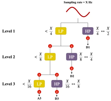
A signal is represented as a set of scaled and translated versions of a mother wavelet which is discussed more in detail in the work of Ngui et al. [21]. When an appropriate mother wavelet is chosen Low Pass (LP) and High Pass (HP) filters can be derived in order to extract the approxi-mation and detail coefficients. The signal to be analysed is filtered through these filters in order to separate the frequency content, the output of the LP filter is the approximation coefficients while the output of the HP filter is the detail coefficients; both of these outputs are downsampled by a factor of two. This process is repetitively done until stopped by some criteria or because there are no more samples left to filter. The process is done with a filter bank setup, where the approximation coefficients are iterated through the filters which are connected in series, Figure 5 shows the process of DWT with filtering up to decomposition level 3.

(16)

Figure 5. An example of how to apply DWT with decomposition level 3 on a signal which has been sampled with a rate of X Hz. The HP filter outputs the detail coefficients while the LP filter gives the approximation coefficients which are used for the following decomposition level. Note that after each level the signals are downsampled by a factor of two and the frequency range is changed due to filtering [22].

A visualisation of the frequency sub-bands can be shown below in figure 6 based on the DWT with a decomposition level 3 which is shown above in Figure 5.

Figure 6. Visualisation of the frequency sub bands when performing DWT on a signal with decom-position level 3; the splitting of the frequency spectrum can be continued for higher decomdecom-position levels [18].

These coefficients can be used further on to reconstruct and represent the original signal as a set of features. The local representation in both the time and frequency domain makes DWT a useful tool for detecting transients in a signal, as discussed in the work by the authors Abed and Mohammed [23]. Here, DWT was used to detect internal faults in transformers when analysing current signals. Similar work has been done by Rumkidkam and Ngaopitakkul [24], where the

(17)

approximation and detail coefficients were compared and analysed when investigating the current behaviour of winding to ground faults in a single-phase transformer.

3.6 From raw data to a set of features

As mentioned in section 3.3 12 signals are measured simultaneously and stored when a trigger criterion is fulfilled. For transformer data, it is of interest to analyse multiple time-series signals since there are correlations between the signals that are collected from a transformer [25]. Methods for extracting and combining features from multivariate time-series are discussed by Mörchen [26] where features were extracted from multiple time-series signals from different problem domains such as power demands. Multivariate time-series is the format of the ABB data since two variables are recorded over time, voltage and current across all six transformer phases. In the work by Mörchen, features were extracted from multiple time-series with two different methods: Discrete Fourier Transform (DFT) and Discrete Wavelet Transform (DWT). DWT showed the best results in terms of classification error percentage when classifying multivariate time-series containing known classes using K-means clustering method. Both DFT and DWT produces a number of coefficients that is increased depending on the frequency content and the length of the signal. Mörchen goes on to suggest a method to decrease the number of coefficients in order to lower the feature dimensionality and still maintain the important signal characteristics. By calculating the energy sum of the signal coefficients, it is feasible to evaluate and remove coefficients that show low importance for the purpose of capturing the signal characteristics.

3.6.1 Feature extraction

Depending on the feature extraction method and domain, the interpretation of the results will differ. For example, the max value of a voltage signal in the time domain compared to the max value of the same voltage signal in the frequency domain will give different information regarding the characteristics of the signal. Table 2 is a list of generic feature extraction methods that can be used in both time and frequency domain depending on what information one is pursuing. xi

denotes the signal, i represents index where the length of this signal is N. Table 2 shows a variety of different features and the corresponding extraction definitions that are possibly useful depending on what information is considered discriminating for the events within the data subset. Features such as max peak, min peak, peak-to-peak, and variance are beneficial when analysing how are really good indicators finding transients and outliers. However, the coefficient of skewness, kurtosis, variance, and standard deviation are useful methods for analysing the distribution of the different sub-bands and could contain useful information regarding the frequency behaviour. Features such as arithmetic mean, mean absolute value, root mean square and simple square integral are beneficial when looking at the amount of content available in the different sub-bands. All of the suggested features must be iteratively evaluated in order to find the most descriptive combination of features for clustering similar events within the data subset.

(18)

Table 2: Generic feature extraction methods for time-series.

Feature extraction method Definition Reference

Arithmetic mean 1 N N X i=1 xi [27] [28]

Mean absolute value

v u u t 1 N N X i=1 |xi| 2 [27] Median              xN/2 2 if N is odd xN/2+xN/2+1 2 if N is even [29] [28] Variance 1 N − 1 N X i=1 (xi− ¯x)2 [27] [30]

Root mean square

v u u t 1 N N X i=1 x2 i [27] [31] [28]

Max peak max(x) [28]

Min Peak min(x) [28]

Peak - Peak max(x) − min(x) [28]

Simple square integral

N

X

i=1

|xi|2 [27] [26]

ithpercentile pi(x) [32] [28]

Crest factor max(x) − min(x)

RM S [33]

Modified crest factor p99(x)

p70(x) − p30(x) [33] Coefficient of skewness m3/m 3/2 2 where mr= 1 N N X i=1 (xi− ¯x)r [32] [28]

Coefficient of kurtosis m4/m22 where mr=

1 N N X i=1 (xi− ¯x)r [32] [28] Standard deviation v u u t 1 N − 1 N X i=1 (xi− ¯x)2 [27] [28]

(19)

3.6.2 Feature selection

It is shown that feature selection has an effect on the performance of learning algorithms, selecting fitting features have various advantages, such as decreasing the computational time and space cost and improving cluster quality; Li et al. [34] discusses the benefits more thoroughly. Dimensionality reduction of the features is beneficial when working with a large data set; from there the data is in a form that can be more efficiently processed by different methods, for instance Machine Learning (ML) algorithms. Vazquez-Chanlatte et al. [35] discusses how ML can be used to tackle large amounts of time-series data; initially, the data is pre-processed and transformed into the feature space and thereafter utilised by ML algorithms. ML algorithms can search for correlations between the features which might give vital insight into a set of data and the quality of the selected features. When selecting features it is important to consider what is necessary to preserve, Laplacian score is a method which is studied by He et al. [36] for this purpose; the feature selection method is based on the evaluation of the features locality preserving power where it is considered beneficial to preserve the neighbourhood structure in the given feature space; the higher the preserved power the lower the Laplacian score is for that feature. Based on the given score it is feasible to sort the features and select a set of features which have the lowest score.

The Laplacian score consists of four steps as specified by He et al. [36] and Li et al. [34], and can be seen below.

1. Construct graph G which is the nearest neighbour graph consisting of all the objects. An edge is then placed between objects that are close to each other in the given feature space. This is done because the method is unsupervised; if labels were available then an edge would be placed between the observations that are under the same label.

2. By viewing the graph G the weight matrix S is created such that if object i and j are neighbours then the element in matrix S corresponding to these objects is set as shown in Eq. 2, otherwise set S(i, j) = 0; t is a pre-defined constant.

S(i, j) = e−kOi−Ojk

2

t (2)

3. The weighted matrix is used to calculate the diagonal matrix D as shown in Eq. 3. It is then used to calculate the Laplacian matrix L for all objects, also referred to as graph Laplacian where L = D − S. D(i, i) = n X j=1 S(i, j) (3)

4. Finally, the Laplacian score Lr is calculated for feature r denoted as fr as show in Eq. 4

where 1 = [1, ..., 1]T. ˜ fr= fr− frTD1 1T_D11 Lr= ˜ fT rL ˜fr ˜ fT rD ˜fr (4) 3.6.3 Feature reduction

Working with high dimensional data is not necessarily beneficial for clustering purposes, the feature set can contain irrelevant information that do not benefit the clustering and increase the compu-tational time [37], [38]. An approach discussed in the work by Lou et al. [39] for reducing the dimensionality is Principal Component Analysis (PCA), an unsupervised method that has proven to be efficient in regards to computational time. PCA is often described as one of the most popular

(20)

unsupervised algorithms since it preserves the variance of the feature set [40]. It is originally a dimensionality reduction algorithm, but has proven to be valuable as a method for visualisation, ML algorithm optimisation, and feature extraction as well. The purpose of PCA is to linearly transform the selected features to a new compressed feature set in a smaller subspace; this method is beneficial when working with data that lacks class labels. One disadvantage is the loss of inter-pretability when examining the new features and the clusters based on these features; this problem requires linking the features with the original data when interpreting. In the work of Boutsidis et al. [41] a dimensionality reduction method for k-means clustering is studied. One of the discussed approaches is random projections which is a method for constructing a set of artificial features from the original features while preserving the Euclidean distance for object pairs. The method projects the features onto a subspace; this proved to effectively reduce the number of features with a low computational cost.

3.7 Clustering

Analysis of time-series data is a subcategory of signal processing concerned with data points mea-sured over a time span. Several methods for clustering these types of signals exist, with different advantages and disadvantages depending on the underlying data and application itself. According to Sheikholeslami et al. [42] four categories of clustering algorithms are normally cited, while Han et al. [43] mention five categories. Discussed by Sheikholeslami et al. are partitioning clustering algorithms, hierarchical clustering algorithms, density-based clustering algorithms, and grid-based clustering algorithms. Han et al. as well as Warren Liao [44] additionally mention a fifth cat-egory which is model-based clustering. Of these, partitioning, hierarchical, density-based, and model-based clustering will be discussed briefly in the following sections due to their prevalence in related literature [45], [46], [47]. In a review conducted by Aghabozorgi [48] et al. partitioning and hierarchical clustering algorithms represents a majority of the approaches selected for clustering time-series data, and will thus be focused on further.

3.7.1 Partitioning clustering algorithms

Partitioning clustering split the given data set with n objects into a known number of groups k. Each group must contain at least one object, and the number of groups must be less than or equal to the number of data objects, i.e. k≤n. The groups can be either crisp if the data objects themselves are only part of one group, or they can be fuzzy if the data can be part of several groups with different membership degrees. Saket and Pandya [49] identify a few popular partitioning methods including k-means, Partition Around Medoids (PAM), Clustering for LARge Applications (CLARA), and Clustering for Large Applications based on RANdomized Search (CLARANS). These are all crisp clustering algorithms, however fuzzy counterparts to them exist such as the fuzzy c-means and the fuzzy c-medoids methods. A short description of the crisp algorithms follow below:

K-means clustering

K-means starts with an initial approximation for the k centroids; these are either randomly created or randomly selected from the data. A centroid itself is the mean centre of an object, in this case a cluster, and does not have to be a point within the cluster itself. Each data point in the set is then clustered to a centroid with the nearest distance. In the second step, the centroids of the clusters are updated using the mean of the data inside the cluster itself. This iterates until a termination criterion is met [50], such as a maximum number of iterations or a convergence of the distance to the clusters’ centroids. The k-means algorithm has a time complexity of O(nki), where n represents the number of objects, k is the number of clusters and i represents number of iterations. Advantages of using k-means are that it creates very tight clusters, and is faster than many other methods such as hierarchical clustering. Disadvantages include the risk of becoming stuck in local minimums, as well as the difficulty of guessing the value of k.

(21)

PAM

The k-medoids algorithm Partition Around Medoids (PAM) is similar to k-means, but one that calculates initial medoids instead of centroids. This method was first proposed by Kaufmann and Rousseeuw [51], [52]. A medoid is a member of the data set that is the most centrally located, unlike a centroid which does not have to be a member of the data set. This data point is then swapped with a random non-medoid, and the cost of this swap is calculated. If cost is positive, then the swapping continues until no change occurs. This is a robust method against outliers in the data, however, it suffers from a high time complexity of O(ik(n − k)2_{) and as a result does not}

fit well with larger data sets [53], [54]. CLARA

CLARA was created by Kaufmann and Rousseeuw [55] as an extension of the PAM method in an attempt to be more suitable for larger datasets. It is less computationally heavy since it randomly sub-samples the data sets, and incorporates PAM in that it uses it to find the medoids within the sampled set itself. The time complexity of CLARA is O(ks2_{+ k(n − k)), where s is the sample}

size. This is an improvement when compared to the PAM algorithm. A problem with this method is that it can end in a local minimum since the best-suited medoids have the risk of not getting selected in the samples, thus its efficiency depends on the sample size according to Ng and Han [54]. CLARANS

Saket and Pandya’s analysis of CLARANS claims that it is a method that is more suitable for data sets with higher dimensionality as well as having increased efficiency. CLARANS too uses PAM for the sampling of the data, but it does not restrict its search, which is randomised, of a minimum node to a particular subgraph. This makes it more effective than both CLARA and PAM, something that was proven by Ng and Han [54] through experimental testing. A disadvantage of this method is that it is computationally heavy with a time complexity of O(n2_{), where n is the}

number of data points [49], and that the quality of the clustering is heavily dependant on how many neighbours are examined [54]. For the algorithm, when given a dataset containing n objects, finding k medoids in this set can be thought of as exploring a graph, denoted Gn,k, where every

node in it could be a solution. A node in the graph is defined as a set of k objects implying that these are the chosen medoids. The nodes can be what is denoted a neighbour to another node if their two respective sets diverge by at most one object. Each of these nodes is a representation of a clustering. This means that every node has a cost, which is the total distance, or divergence, between the objects associated with these nodes and the chosen medoids that they belong to. The total cost of replacing the current node with a new medoid, that is, the difference in cost between two adjacent nodes, can be calculated according to Eq. 5. T Cmp represents the total cost, while

Cjmp is the cost of swapping a selected object with a non-selected object, and can be defined in

four different ways as discussed further by Ng and Han [54]. T Cmp=

X

j

Cjmp (5)

CLARANS is an iterative algorithm, and for each passing a collection of nodes are randomly set to allow for the exploration of new medoids. If the cost calculated by Eq. 5 is lesser for a neighbouring node than for the current node under inspection the neighbour is set as the new current node. If the cost is greater or equal, the current node is identified as a local optimal point. This practice is continued iteratively in order to identify new and better optimal points.

3.7.2 Hierarchical clustering algorithms

Hierarchical clustering groups the data objects in a tree structure; an example of this can be seen in Figure 7. This clustering algorithm can be divided further into two types, which are agglomerative hierarchical clustering and divisive hierarchical clustering. Agglomerative clustering begins by placing all data objects as separate clusters and then iteratively merges them. Divisive clustering is the opposite in that it starts with one cluster and then dividing it up iteratively. A disadvantage

(22)

of hierarchical clustering is that the structure is very rigid, and cannot be altered once a grouping or a division has taken place [45]. An advantage is, however, that hierarchical algorithms do not rely on the variable k, denoting the number of clusters, being specified beforehand.

Figure 7. Tree structure for hierarchical clustering. Two different groupings are performed, one where k=2 and one where k=5.

Agglomerative clustering

In agglomerative clustering, also denoted AGNES (Agglomerative Nesting) or bottom-up cluster-ing, each data object is viewed as a cluster consisting of only that object. These clusters are subsequently grouped with each other until only one large cluster remains, or a set requirement is fulfilled. The grouping is done by choosing pairs that have the smallest within-cluster dis-similarity [56]. The final product of this is denoted a dendrogram, also known as a tree-model. Hierarchical clustering has a complexity of O(n3_{) for standard agglomerative clustering, which is}

slower than many of the partitioning algorithms. Divisive clustering

Divisive clustering has not been as exhaustively researched as agglomerative clustering, but could hold an edge over it in regards to creating comparably few clusters [56]. Divisive clustering, also denoted DIANA (DIvisive ANAlysis) or top-down clustering, starts out the other way around with all data objects in one large cluster. This is split in a recursive manner with an algorithm that uses the most heterogeneous cluster which forms two new, smaller clusters. These new clusters should have the highest between-group dissimilarity or alternatively, the cluster with the largest diameter is selected for separation [56]. The final output of the algorithm can here too be represented as a dendrogram. Divisive hierarchical clustering has a time complexity of O(2n_{) with exhaustive}

search [47], [57]. This makes the algorithm unsuitable for large datasets since the complexity will grow as the number of calculations performed on the data increases.

3.7.3 Model-based clustering

This family of clustering techniques is usually applied in one of two ways; either with a neural network technique or a statistical technique. According to Warren Liao [44] competitive learning and self-organising feature maps are two common methods using the neural network technique. Disadvantages with model-based clustering include its slow computation which makes it non-ideal for big data sets [58].

3.7.4 Density-based clustering

Density-based clustering methods work by the principle of a density criteria, in which the clusters themselves are areas containing high-density data objects while the areas in between them are of

(23)

low density. In the analysis of clustering algorithms by Sheikholeslami et al. [42], two density-based methods are discussed. These are the Difference-Of-Gaussian (DOG) based clustering technique and the Density-Based Spatial Clustering of Applications with Noise (DBSCAN). DBSCAN has some advantages such as the ability to filter out noise in the data, but both this method as well as the DOG-based technique suffers from high time complexity. Another example of a density-based clustering method is the Quality Threshold (QT) algorithm, which has a time complexity of up to O(n5) [59]. Denton [60] presents a kernel-density-based clustering method that shows promising results when compared to other density-based algorithms, as well as the k-means algorithms, but is only focusing on smaller data sets.

3.8 Similarity measurement

Since clustering of time-series data depends heavily upon the intra-class similarity between the data objects, one important part of clustering is the method used to compare two waveforms, or time-series [61]. Esling and Agon [62] first makes one distinction for distance measurements and identifies two groups which are elastic measurements and lock-step measurements; these are detailed more in the following sections. The authors further define four groups of distance measurements, these are: edit-based, feature-based, structure-based, and shape-based. Structure-based measures can be separated into model-based and compression-based techniques. Aghabozorgi [48] et al. observe that one of the most commonly used methods for time-series clustering are shape-based methods. 3.8.1 Lock-step measurements

Lock-step measurements produce a linear alignment of time-series data. As such it matches the i th point of an arbitrary time-series X with the i th point in time-series Y, as is the general case of all lock-step measurements.

Minkowski distance

The Minkowski distance measurement is a shape-based lock-step measurement, and the definition for it can be seen in Eq. 6, as stated by Chouikhi et al. [63]. In the equation, D(X,Y) is the distance between two time-series X and Y, where i is each corresponding data point within the series, and | denotes absolute value.

D(X, Y ) = (

l

X

i=1

|X[i] − Y [i]|p₎1_p ₍₆₎

When the parameter p is equal to 2, the generalised form becomes the special case called the Euclidean distance, as defined in [64]. Another common special form is when p is equal to 1, which is denoted the Manhattan distance. These two forms can be seen in Eq. 7 for Euclidean distance and Eq. 8 for Manhattan distance.

Deuc(X, Y ) = ( l X i=1 (X[i] − Y [i])2)12 (7) Dman(X, Y ) = l X i=1 |X[i] − Y [i]| (8) Cosine similarity

The Cosine similarity measurement [43] is a shape-based method that measures the difference in orientation between two time-series, and is defined as:

Dcos(X, Y ) = 1 −

XY

kXk kY k (9)

where X and Y are the two series, and kXk and kY k are the Euclidean norms for time-series X and Y respectively. The product of the two norms compute the cosine of the angles

(24)

between the time-series, and a value of 0 denotes an orthogonality between them while a value of 1 denotes a perfect match.

3.8.2 Elastic measurements

Elastic measurements takes two time-series sequences and warps them in a non-linear manner to account for possible deformations in their structure. The measurement method produces a non-linear alignment of two time-series, which means that similar time-series can match no matter the phase shift, i.e. that it can do a flexible comparison. This also makes the measurement more robust in handling outliers. A visualisation of the difference between lock-step and elastic alignments can be seen in Figure 8 and 9.

Figure 8. Example of lock-step linear align-ment, where the i th data point in time series X matches the i th data point in time series Y.

Figure 9. Example of elastic non-linear align-ment, where only the first and last data points in time series X have to match the first and last data points in time series Y.

Dynamic Time Warping

DTW is a shape-based elastic measurement. This distance measurement was first defined in 1978 by Sakoe and Chiba [65], however, the definition used in this work is the notation used by M¨uller [66] with altered parameter names for the sake of conformity. The definitions for the DTW distance can be seen in Eq. 10 and 11. In Eq. 10, cp(X, Y ) is the total cost of what is denoted a

warping path p between two time-series X and Y, where each element of the sequence is denoted xnl and yml respectively. L is the length of the warping path. The optimal path between the two

time-series is denoted p∗, and has the least total cost of all paths. Cost is computed as the sum of absolute differences, for each matched pair of indices, between their values. In Eq. 11 DTW(X,Y) represents the DTW distance between time-series X and Y, and is the total cost of p∗_{. N and M}

is the respective lengths of the time-series X and Y.

cp(X, Y ) := L

X

l=1

c(xnl, yml) (10)

DT W (X, Y ) := cp∗(X, Y ) = min[c_p(X, Y )| p is an (N,M)-warping path] (11)

Since the number of paths can grow exponentially they are restricted by five types of condi-tions: boundary conditions, monotonic conditions, continuity conditions, the adjustment window condition, and the slope constraint condition. DTW has been proven to be an effective method of similarity measurement for clustering of time-series data, such as in the work by Keogh and Ratanamahatana [67] where exact indexing of DTW is explored. The standard DTW similarity measurement has, however, a debatable performance when it comes to larger data sets since the computational cost is quite high (O(MN)) as remarked by M¨uller [66], however, optimised versions exist such as [68], [69].

(25)

3.9 Quality analysis

Thorough analysis and evaluation of the quality of the created clusters are necessary so as to verify that they are adequately formed. Three areas are identified by Theodoridis and Koutroumbas [70] for cluster validity analysis. The first type is the external criteria, which estimates to which de-gree the created clusters match externally provided labels, as well as the possibility to establish a connection between the data itself and a predefined clustering structure. Using external measure-ments, it is possible to set a specific value for the parameter k, specifying number of clusters to be used in the clustering algorithm that require a beforehand specified parameter value for this. The second type of analysis methods is the internal criteria, which estimates the goodness of the structure itself without the use of any external labels, meaning that the data is only analysed in relation to itself. This type of method is often used to instead estimate the number of clusters k to input to clustering algorithms. The final type is the relative criteria, by which it is possible to compare a clustering structure with other structures. The numerical implementations of these are often referred to as external-, internal-, and relative indices. A thorough overview on different types of internal and external validation criteria for clustering is presented by Desgraupes [71]. A selection of some of these are presented in the following sections along with information regarding the respective groups of methods.

3.9.1 External criteria

All external criteria methods follow the same underlying structure in that they make use of a confusion matrix that symbolises data point pairs and whether they belong to the same cluster or not as defined by a clustering partition and a reference partition. For all methods a low or zero value for the index in question indicates a low or zero relationship between the clusters and the reference point, while a higher value indicates a higher correlation between them. Four categories are distinguished by Desgraupes [71]:

1. Two data points belong to the same cluster as confirmed by both partitions

2. Two data points belong to the same cluster as confirmed by the clustering partition, but not the reference partition

3. Two data points belong to the same cluster as confirmed by the reference partition, but not the clustering partition

4. Two data points belong to different clusters, as confirmed by both partitions

Three types of external criteria methods for quality validation using external reference points from Desgraupes overview are discussed by Riyaz and Wani [72]. As mentioned, these methods follow the above structure in grouping the data pairs being compared, and are the Rand index, the Jaccard index, and the Fowlkes-Mallows (FM) index. The Rand index is described as being capable of performance assessment of both classifiers and created clusters, while the Jaccard index is an indicator of good pairs of data seen from the total amount of both good and bad data pairs by excluding a so-called ”neutral term” from the evaluation. FM index evaluates the relationship between the created clusters and part of the data set aside from the clustering process.

3.9.2 Internal criteria

Many of the clustering methods discussed require a specified value for the variable k, denoting the number of clusters. This value is often unknown and has to be set by the user. Without prior information about the system, this value is estimated through the use of internal criteria methods. These are concerned with two concepts: cohesion and separation. Cohesion is a measure on how tight a cluster is or an estimation of the relationship degree of the data within a cluster. Separation, however, is a measure on how spread out the clusters are, or their distinction from each other. These are also known as the intra-cluster and inter-cluster distances. The intra-cluster distance is a measurement of the distance between the medoid (in the case of medoid-based algorithms) and the objects that belong to it. The inter-cluster distance is a measurement of the distance between the medoids of any two clusters. Many methods for this exist, and from studies performed by both

(26)

Nisha and Kaur [73] as well as Charrad et al. [74] a selection of the internal indices as detailed by Desgraupes [71] are compiled in Table 3.

Table 3: Clustering evaluation indices.

Index Distance measurement Reference

C-index Intra [75]

Calinski-Harabasz Score Intra/Inter [76]

Davies-Bouldin Index Intra/Inter [77]

Dunn Index Intra/Inter [78]

Error Sum of Squares Intra [73]

Silhouette Index Intra [79]

Internal measurements often lie between different intervals and their respective criteria differ. For some methods a value close to zero is desirable (or an otherwise minimisation within the set interval), while for other methods a higher value for the index indicates a tighter clustering. C-Index

The C-index was first proposed by Dalrymple-Alford [75] in 1970. It measures the within-cluster similarities and the ratio between the minimum and the maximum of these. The index can be calculated as:

cindex = Du − (r × Dmin) (r × Dmax) − (r × Dmin)

(12) where Du is the total summation of all the cluster distances, r is the amount of intra-cluster distances, and Dminand Dmaxrespectively is the minimum and maximum distances within

the group. The index value itself is bounded between [0,1] meaning it is a normalised estimator, where lower values denotes a good clustering, while higher values denote a worse clustering. The time complexity of the C-index is O(N2_{(n + log}

2N )) [80], where N is the number of data objects

and n represents the size of the vector of distances. Calinski-Harabasz Index

The Calinski-Harabasz (CH) Index as defined by Calinski and Harabasz [76] in 1974 and can be calculated as:

CH(k) = BGSS/(k − 1)

W GSS/(N − k) (13)

where BGSS denotes the between-group sum of squares, WGSS denotes the within-group sum of squares, N is the number of data points, and k the number of clusters. The definition for BGSS is: BGSS(k) = k X l=1 n X j=1 |Cl| (¯clj− ¯xj)2 (14)

where Cj denotes the amount of objects in cluster Cj and ¯clj denotes the j th midpoint of

cluster l. Parameter ¯xj denotes the j th midpoint of all objects, while n represents the size of the

object itself. WGSS can be defined similarly as:

W GSS(k) = k X l=1 X i∈Cl n X j=1 (xij− ¯clj)2 (15)

where Cl denotes cluster l, xij denotes the j th index of object i, and ¯clj is the j th midpoint

(27)

has a time complexity of O(nN ) [80] where n correlates to the size of the matrices defining BGSS and WGSS and N is the number of data objects.

Davies-Bouldin Index

The Davies-Bouldin Index (DB Index) defined by Davies and Bouldin [77] is similar to the CH Index in that it also bases its measurements on within-group and between-group differences. For every created cluster the distance between it and the other is calculated. The average of the largest distance for each cluster results in the DB Index. This means that it is desirable with a DB Index that is as small as possible, and thus the goal is to minimise this function as close to zero as possible. The index calculation is:

DB(q) = 1/k k X r=1 maxs,r6=s Sr+ Ss dr,s (16) where k is the number of clusters. The variable dr,s represents the distance between the

midpoints of the clusters currently being examined, and maxs,r is the largest distance between

two clusters. Sr is a dispersion measurement for cluster r and Ss is a dispersion measurement

for cluster s respectively, where r, s = [1, 2, 3, ..., q] with a length of q. Dispersion measures the stretching of distribution, or in this case a cluster, and the specific measurement used by Davies and Bouldin is defined as

Si=    1 Ti Ti X j=1 |Xj− Ai| q    1/q (17)

where Tirepresents the number of vectors in cluster i and Aiis the centroid of the i th cluster.

The time complexity of DB Index is O(n(k2+ N )) [80], where n is the dimensionality of the sample vectors and N is the number of data objects.

Dunn Index

The Dunn Index was defined by Dunn [78] in 1974. It utilises the relationship between the maximal intra-cluster distance and the minimal inter-cluster distance, and can be calculated as:

Dunn = min1≤i<j≤kd(Ci, Cj) max1≤g≤kdiam(Cg)

(18) where k defines the number of clusters, d(Ci, Cj) defines a dissimilarity between two clusters,

and diam(Cg) is the diameter of cluster g, where 1 ≤ g ≤ q. The diameter itself is the largest

distance between two points within a cluster. Since the Dunn Index measures the ratio of intra-cluster distance over inter-intra-cluster distance a large value is desirable. The time complexity of the Dunn Index is O(nN2) [80], where N represents the number of data objects and n is the distance vector size.

Error Sum of Squares

Error Sum of Squares (SSE) is mentioned by Nisha and Kaur [73] as a suitable method for per-forming cohesion measurement of a created clustering. SSE determines the distance between all objects within a cluster and the mean of the cluster; these distances are summed to form a total value for the differences. This is defined as:

SSE =

n

X

i=1

(xi− ¯x)2 (19)

where xidenotes the object being compared to the mean and ¯x is the mean value of the cluster

(28)

Silhouette Index

Silhouette Index, a method for crisp clustering first described by Rousseeuw [79], is mentioned as being the most popular criterion out of the three described by Nisha and Kaur [73]. Using this method, the quality of the cluster is measured based on the graphical form of it and produces a value that is denoted as a silhouette width. By using this method the cohesion and the separation of the clusters can be measured. The silhouette width s(i) can be defined as:

s(i) = b(i) − a(i)

max(a(i), b(i)) (20)

where a(i) denotes the average within-cluster distance for observation i and b(i) denotes the smallest average distance of observation i to all the objects in the cluster closest to its own cluster. The silhouette value itself is bounded between [-1, 1], where a value of 1 or close to it denotes a near-perfect clustering, a value of 0 or close to it denotes overlapping clusters, and a value of -1 or close denotes bad clustering according to Rousseeuw. The overall time complexity of the Silhouette Index is O(nN2) [80], where N represents the number of data objects and n is the distance vector size.

3.9.3 Relative criteria

Relative criteria methods differ from external and internal measurements in the manner that the target is to select the best set of clusterings in reference to an already defined benchmark. This is generally done by altering the parameters used in the clustering, such as number of clusters used, and comparing the different results.

(29)

4 Related work

The previous section introduces a wide set of concepts that are important in order to understand the work that is done in this thesis. This section is an exhaustive study of the state of the art in related works and the recent advances and research in the field of waveform clustering, as well as the different advantages and disadvantages that the studies highlight. Building from this knowl-edge base an appropriate method for tackling the specific problem at hand was selected.

Analysis regarding the feasibility of online monitoring transformer parameters was carried out by Abeywickrama et al. [1] to investigate the possibility of detecting certain faults in power net-works both short-term and long-term. This work builds upon previous work by the authors [81] detailing detection methods of transformer problems, as well as other work commissioned by ABB Corporate Research [82]. The focus in the recent study was on the detection of short-circuit impedance, power loss, and turn ratio as well as an overlook of the causes of these commonly seen transformer issues. The proposed method can use signals readily available in a control room setup, and implements the commonly used two winding transformer model; from there various transformer parameters are available for analysis. It could be seen that even small variations could be discovered in the monitored parameters. The results show that the suggested method can be used instead of the off-line test since the tolerance limits are comparable to the sensitivity of the suggested method. However, this method of fault detection relies on human knowledge which may lead to a bias towards already known events, which makes it hard to discover patterns that are unexpected.

Power systems create massive amounts of data regarding the stability of the system itself. To be able to analyse this, the relevant information needs to be extracted in an efficient manner. Cluster-ing was used in a study performed by Dutta and Overbye [83], where the QT clustering algorithm was used to gain insight into the system response for a large-scale power system consisting of 16 000 buses for the purpose of visualising transient stability data. Before being able to cluster the data, it was first pre-processed using normalisation. After this, feature extraction was performed on the signals so that a similarity measurement could be achieved; the features consist of frequency and voltage transients. Different measurements were analysed such as the Minkowski distance, the Euclidean distance, Cosine measurement, as well as the Root Mean Square (RMS). The signals displaying similarities were then clustered using K-means clustering in combination with QT to reduce the amount of data for a more simplified process. The method proved to be fast even when working with a large set of data points and could identify data that is important to general system response. More importantly, however, is that the method also displayed a high capacity of identifying outlier data points that could warrant the need for further investigation. The cluster-ing method itself only requires one feature, and because of the nature of the data that has been collected, many more features are available; this requires heavy modification to this type of method. In the research performed by Sun et al. [84] the increasing complexity of power networks which increases the amount of data produced, pressuring the computational speed, and reliability on the Power Grid Dispatch and Control System (PGDCS) is discussed. This complexity is shown to be problematic when emergencies occur on the power grid since the data needs to be sent, received, and processed within a short time span. The suggested method is to cluster the different processing units in order to improve the computational capability and solve the existing bottleneck problem. The size of the clusters are also addressed since the increase of size could lead to poor data synchro-nisation and high schedule cost which is mentioned but not investigated in the work by the authors. Large-scale blackouts on the electrical grid is a risk which is problematic and hard to predict. A method to combat this issue is addressed by Tomin et al. [85] where an intelligent unsupervised clustering ensemble-based system is implemented. Large amounts of data are collected from the power system and thereafter go through a feature selection where the violated safety parameters are chosen with the Non-linear Iterative Partials Least Square (NIPALS) algorithm in order to construct principal components for feature selection. The data is processed through three un-supervised algorithms; these are Fuzzy c-means, Kohonen map, and K-means. Each technique

Waveform clustering - Grouping similar power system events

V¨

aster˚

as, Sweden

Thesis for the Degree of Master of Science in Engineering - Robotics

30.0 credits