Using METRIC to Estimate Surface Energy Fluxes over an Alfalfa Field
in Eastern Colorado
Mcebisi M. Mkhwanazi1 and José L. Chávez
Department of Civil and Environmental Engineering, Colorado State University
Abstract. The ability to estimate surface energy fluxes using remote sensing methods has enabled the determination of evapotranspiration over a large area with less cost. Several models that employ the energy balance method have been developed. The model discussed in this paper is the Mapping Evapotranspiration at high Resolution with Internalized Calibration (METRIC). It estimates net radiation (Rn), soil heat flux (G), sensible heat flux (H), and then determines latent
heat flux (LE or ET) as a residual. Landsat 5 TM and Landsat 7 ETM images for the 2010 alfalfa growing season near Rocky Ford, CO, were processed and analyzed using Erdas Imagine 2010 Software. The accurate estimation of Rn and G is important as these two determine how much
energy is available to be partitioned into H and LE. Hence, the focus on evaluating Rn, G and ET in
this study. The results obtained from the processed images were compared with actual fluxes measured by instruments installed in the alfalfa field and performance indicators for each flux were
determined. For Rn, the Mean Bias Error (MBE) was 17.8 W m-2 (3.3%), and the Root Mean
Square Error (RMSE) was 22.1 W m-2 (4.1%), the Nash-Sutcliffe coefficient of Efficiency (NSE)
value of 0.53 and R2 of 0.84. The G MBE was -3.0 W m-2 (-5.8%), RMSE of 14.2 Wm-2 (27.6%),
NSE value of 0.79 and R2 of 0.96. Hourly ET resulted with an MBE of -0.08 mm h-1 (-10.3%) and
an RMSE of 0.14 mm h-1 (17.6%), NSE of 0.71 and an R2 of 0.83. It was observed that the
estimation of G had larger errors under smaller biomass surface conditions (e.g., when the alfalfa had just been harvested). However, overall the remote sensing model estimated well the heat fluxes and it seems to be suitable for applications at regional scales in hydrology studies.
1. Introduction
In most semi-arid and arid places, irrigation has been known to claim the larger portion of the water resource. With other sectors demanding more water (e.g., urban, industry, tourism), it is becoming necessary to improve the management of irrigation water, which would involve the accurate estimation of crop water consumptive use otherwise termed evapotranspiration. Evapotranspiration (ET) is an essential component of the field water balance as well as the regional hydrologic cycle and it is a significant consumptive use of precipitation and water applied for irrigation on cropland (Paul et al., 2011).
Several methods are being used to measure or estimate ET, one of them being the weighing lysimeter method that measures directly the water used by crops (vegetation). Using reference ET to estimate crop ET by using crop coefficients as explained by Doorenbos and Pruitt (1977), the Bowen ratio surface energy method and the eddy covariance (EC) are other methods used to estimate evapotranspiration. The Bowen ratio
1 Civil and Environmental Engineering Department Colorado State University
Fort Collins, CO 80523 Tel: (970) 818-1159
depends on sensor accuracy to measure small differences in air humidity (Bastiaanssen et al., 2005). There are also assumptions employed for this method, e.g. that the turbulent transfer coefficients for heat and vapor are identical, and also that there are no horizontal gradients of temperature and humidity, the latter assumption would require an adequate fetch to be valid. The eddy covariance method is usually affected by energy balance closure error (Twine et al., 2000). This characteristic of the EC method may result in non-accurate estimation of heat and vapor fluxes under certain conditions.
Remote sensing (RS) images and methods can be used to indirectly estimate spatially distributed ET. One of the RS techniques makes use of the land surface energy balance (EB) equation.
Rn = LE + G + H (1)
Where all the terms of the EB are expressed in energy units (W m-2).
In this RS technique, satellite sensed land surface radiances, in different band widths are converted into surface properties such as albedo, vegetation indices, surface emissivity, and surface temperature. Then the RS model uses all these properties, parameters, and variables to estimate the various components of the EB model (i.e., Rn, H, G) then LE as a
residual (Gowda et al., 2008).
Several models have been developed; Surface energy balance algorithm for land (SEBAL; Bastiaanssen et al., 1998), Mapping Evapotranspiration with Internalized
Calibration (METRIC; Allen et al., 2007), Remote Sensing of evapotranspiration (ReSET; Elhadad and Garcia, 2008), Analytical Land Atmosphere Radiometer Model (ALARM; Suleiman et al., 2009) and Surface Aerodynamic Temperature (SAT; Chávez et al., 2005, 2010). SEBAL was developed to estimate ET over large areas using satellite surface energy fluxes (Bastiaanssen et al., 1998). It is capable of estimating ET without prior knowledge on the soil, crop, and management conditions (Bastiaanssen et al., 2005). This method has been used widely including the US, Africa, Europe and other parts of the world. METRIC on the other hand is a modification of SEBAL and is based on the same principles, and also making use of the near surface temperature gradient (dT) function as proposed by Bastiaansen (Singh et al., 2008). The use of satellite based EB models has some advantages over the other traditional methods. One of them is that it provides
regional estimates rather than field estimates of ET. Another advantage is that RS methods estimate the actual evapotranspiration, while some other methods use meteorological data to estimate reference ET then estimate actual ET using crop coefficients.
This paper serves to evaluate METRIC, by comparing fluxes estimated using this method (i.e., Rn, G, and LE or ET) with measured fluxes. The aim is to determine how
accurate the model is in estimating the various components of the EB equation over an irrigated alfalfa field in eastern Colorado.
2. Material And Methods 2.1 Study Area
This study was carried out at the Colorado State University (CSU) Arkansas Valley Research Center (AVRC) near Rocky Ford, Colorado (U.S.A.) with geographic
coordinates being 38°02’N, 103°41’W, and the area’s elevation 1,274 m above sea level. The field (160 m x 250 m) under study was cropped with alfalfa, and had a weather station on site. A large monolith weighing lysimeter (3 x 3 x 2.4 m) was located in the middle of the field. The alfalfa was irrigated through a furrow irrigation system using siphons and a head ditch. As part of the instrumentation in the field, there was a net radiometer, Q7.1 net radiometer (REBS, CSI, Logan, Utah, U.S.A.), two infra-red thermometers (IRT Apogee model SI-111, CSI, Logan, Utah, U.S.A.) to measure the crop radiometric surface
temperature, soil heat flux plates (REBS model HFT3, CSI, Logan, Utah, U.S.A.) buried in the ground at the lysimeter locations, with depths ranging from 8 to 15 cm, along with soil temperature and soil water content sensors, for the estimation of soil heat flux at the ground surface.
2.2 Landsat Datasets and Processing
Landsat 5 Thematic Mapper (TM) and Landsat 7 Enhanced Thematic Mapper Plus (ETM+) cloud free satellite images (Path 32, Row 34), were obtained from the United States Geological Survey (USGS) Earth Explorer site
[(http://edcsns17.cr.usgs.gov/NewEarthExplorer/)] for the 2010 crop growing season. The acquisition dates were May 6, May 22, July 9, August 10 and August 26 for Landsat 5 TM. For Landsat 7 ETM+, images were acquired for the following dates: June 15, July 1, August 2, and August 18. The images were processed using the ERDAS Imagine 2010 software (ERDAS, Norcross, Georgia, U.S.A.).
2.3 Remote Sensing based METRIC algorithm
METRIC estimates ET through the land surface energy balance (EB) method, using remotely sensed surface reflectance in the visible and near infra-red portions of the
electromagnetic spectrum. The radiometric surface temperature is also calculated using the infra-red thermal band. The approach is to convert satellite sensed radiances into land surface characteristics that include surface albedo, vegetation indices, surface emissivity, and surface temperature. These are then used to calculate the various components of the energy balance; Rn, G, and H, then LE estimated as residue of the land surface balance as
given in Eq. 1. How these components are determined is explained briefly in this paper, and a more detailed explanation can be obtained in Allen et al. (2005, 2007).
2.3.1 Net radiation
Net radiation is calculated by summing up the net shortwave radiation and net longwave radiation, and is given by equation 2 below:
Rn = (1 – α) Rs + εaσTa4 – εoσTs4 – (1-εo) εaσTa4 (2)
Where Rs is incoming shortwave radiation which is based on solar constant (Gsc = 1,367 W/m2), the cosine of incidence angle (cosΘ), the inverse squared relative earth-sun distance (dr) and atmospheric transmissivity (τ ), and the transmissivity being a function
of the area’s elevation above sea level. The other components of equation 2 are the longwave portion which includes energy emitted by the surface (Lout) and the longwave
emitted from atmosphere towards the surface (Lin) and the reflected longwave (Lrefl.). 2.3.2 Soil Heat Flux, G
The soil heat flux is the rate of heat storage into the soil and vegetation due to conduction (Gowda et al., 2011). Different empirical equations have been developed, based on extensive soil heat flux measurements made in experimental fields (e.g., Singh et al. (2008), Bastiaanssen et al. (1998)). The one used in this study (Eq. 3) was published by Bastiaanssen et al. (1998).
G/Rn = Ts/α (0.0038α + 0.0074α2) (1 – 0.98NDVI4) (3)
Where α is the surface albedo, which is the ratio of reflected to incident solar incident at the surface. Ts is the radiometric surface temperature (K) which is obtained by making use
of the thermal band of the electromagnetic spectrum. NDVI is the Normalized Difference Vegetation Index, and is computed using the reflectance of bands 3 and 4 in Landsat 5 and 7 which are the red and near infra-red bands respectively.
2.3.3 Sensible Heat Flux, H
The basic calculation of H is by using the equation:
H = ρaCpa (To – Ta)/rah (4)
Where ρa is air density (kg m-3), Cpa is specific heat of dry air (~1004 J/kg/K), Ta is average
air temperature (K), To is the average surface aerodynamic temperature (K), and the rah
term is the surface aerodynamic resistance (s m-1). The To is not measured and may be
difficult to estimate, thus some methods end up using the radiometric surface temperature (Ts). However the assumption that aerodynamic temperature is equivalent to the
radiometric temperature may result in errors in the estimation of H. This is because there may be differences between To and Ts especially over heterogeneous surfaces. In
METRIC, that challenge is allegedly solved by introducing a dT function which replaces (To – Ta) in Eq. 4. The dT is the temperature difference at two levels (i.e., near surface at
0.1 m and at 2 m).
To determine dT, two extreme pixels, a wet and a dry pixels are selected. In the
selection of a wet pixel, a pixel that has a low temperature is selected, with the assumption that the low temperature is as a result of the available energy being used to evaporate (or evapo-transpirate) water instead of warming the air above the surface, therefore suggesting wet conditions. A well vegetated area (pixel) having relatively cool temperature is then selected. The dT associated with that pixel is given as:
dTcold = (Rn – G – 1.05 × ETr) × rah / (ρair × Cpa) (5)
ETr being the alfalfa reference ET computed with weather station data from an alfalfa
field. The standardized ASCE Penman-Monteith equation for alfalfa reference ET (ASCE-EWRI, 2005) is used for the calculation of ETr. The hourly ETr, for the satellite overpass
well-established field of alfalfa can occasionally have an ET slightly greater than ETr (Allen et
al., 2002).
In the selection of the dry pixel, a high temperature pixel would indicate dry surface conditions. However, care should be taken that man-made surfaces such as highways and buildings are not selected. A dry agricultural area (possibly fallow) would be
recommended (Allen et al., 2005, 2007). This pixel is assumed to have no ET, and would result with a large value of dT (dThot). However, in some cases, especially after a rainfall
event, such an assumption does not always hold and METRIC does consider such a possibility. A daily surface soil water balance (SWB) is recommended for the hot pixel to confirm that ET equals zero, or otherwise be given a nonzero value (the calculated value from the SWB). Once the dry pixel is identified, the value of H can be calculated using Rn
and G from that hot pixel. The dT value can then be calculated using Eq. 6. dThot = H × rah/(ρair × Cpair) (6)
A linear relation of dT to radiometric surface temperature is then assumed and the relationship explained by the use of coefficients “a” and “b” whereby:
dT = aTs + b (7)
where the coefficients “a” and “b” can be found as follows:
2.4 Calculation of Instantaneous ET
The first calculation of H is a preliminary estimate (considering neutral atmospheric conditions), and calculation of H must be repeated (iterative process) considering
atmospheric stability through the use of similarity theory (Monin-Obhukov stability length parameter, L) until the difference in rah computations between two consecutive iterations is
less than 5%. It is important to consider stability as it affects the surface aerodynamic resistance to heat transport that directly affects the value of sensible heat flux (Elhaddad and Garcia, 2008). Once the final values of H are calculated, and having computed Rn and
G, the latent heat flux is then calculated from the general EB equation (Eq. 1) as a residual. This LE computation would represent the instantaneous evapotranspiration at the time of the Landsat overpass.
3. Evaluation Criterion
Several performance indicators were used to evaluate the model in estimating the various components of the energy balance. The coefficient of determination (R2) which
describes the proportion of variance in measured data explained by the model is one of the indicators used. It ranges between 0 and 1, with a value closer to 1 indicating less variance. Other indicators used were the Nash-Sutcliffe coefficient of efficiency (NSE), which ranges between -∞ to 1, with NSE of 1 being the optimal value, and values between 0 and 1 show an acceptable model performance. Also, in this study the Mean Bias Error (MBE) has been used and the Root Mean Square Error (RMSE).
hot cold hot cold dT dT a Ts Ts − = −
b dT
=
hot− ×
a Ts
hot4. Results and Discussion
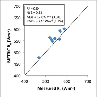
In general, METRIC resulted in good performance in predicting net radiation and soil heat flux. The net radiation was predicted with an MBE of 17.3 W m-2 (3.3%) and RMSE
of 22.1 W m-2 (4.1%), an R2 of 0.84 and an NSE value of 0.53. This compares well with other studies (Paul et al., 2011) and the performance is within the ±5% error which is said to be typical of Rn measurements (Chávez et al., 2009). Figure 1 shows that the model
slightly overestimates the Rn, as most points are just above the 1:1 line.
Figure 1. Comparing METRIC-modeled and measured Rn values.
In the comparison of soil heat flux, the R2 resulted in 0.96, with an MBE of -3.0 W m-2 (-5.8%) and a RMSE of 14.2 W m-2 (27.6%), and the NSE coefficient was determined to be 0.71. This was considered to be a good performance of the model in estimating soil heat flux. A percent bias of more than 40% has been reported in some studies (e.g. Paul et al., 2011).
Figure 2 shows a large discrepancy between estimated and measured G. This
discrepancy occurred on August 26, where METRIC grossly underestimated the soil heat flux, 87 W m-2 versus a measured value 120 W m-2. It should be noted that this was two days after harvesting; therefore there could have been patches of variable biomass presence in the field (very low to low). The heterogeneity in the field could have resulted in the underestimation of G by METRIC since the thermal pixel is very large and averages distributed conditions over the field.
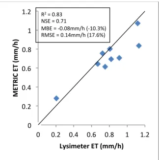
According to the performance indicators, METRIC seemed to estimate ET fairly well; with hourly ET (Fig. 3) having an R2 of 0.83, an MBE of -0.08 mm h-1 (-10.3%), an RMSE
of 0.14 mm h-1 (17.6%), and the NSE coefficient value was 0.71. These results suggest a good level of model performance. The percentage error was largest on August 26. This would have been due to the underestimation of soil heat flux and to some extent to an underestimation of H (not evaluated in this study) as caused by the model’s inability to accurately estimate soil heat flux from heterogeneous surfaces due to patches of low
400 450 500 550 600 650 700 400 500 600 700 ME TRI C Rn (Wm -‐2) Measured Rn (Wm-‐2) R2 = 0.84 NSE = 0.53 MBE = 17.8Wm-‐2 (3.3%) RMSE = 22.1Wm-‐2 (4.1%)
biomass presence. This may have resulted in a higher available energy (Rn – G), and
subsequently the overestimation of hourly ET. Chávez et al. (2009) also made an observation that the percentage error seemed larger for values with low ET rates which also is the case for August 26 in this study.
Figure 2. Comparing METRIC-modeled and measured G.
Figure 3. Comparing METRIC-modeled and Lysimeter-measured hourly ET.
According to the findings of this study with somewhat limited data, it appears that there could be room for improving the soil heat flux model, by Bastiaanssen et al. (1998), by considering low to very low biomass conditions as well as a wide range of soil water content (SWC). In addition, the sensible heat flux model in METRIC should be evaluated
0 20 40 60 80 100 120 140 0 20 40 60 80 100 120 140 ME TRI C G (W m -‐2) Measured G (Wm-‐2) 0 0.2 0.4 0.6 0.8 1 1.2 0 0.2 0.4 0.6 0.8 1 1.2 ME TRI C ET (m m /h ) Lysimeter ET (mm/h) R2 = 0.83 NSE = 0.71 MBE = -‐0.08mm/h (-‐10.3%) RMSE = 0.14mm/h (17.6%)
separately by means of eddy covariance and large aperture scintillometry for instance to assess its accuracy. It is presumed that the H model may have underestimated H under the low biomass conditions in which the G model yielded lower values than measured ones. 5. Conclusions
In this study, METRIC performed very well in the estimation of Rn and G, except for
cases when the alfalfa was harvested and the field displayed low biomass presence. In general, METRIC estimated ET with a relatively low error. However, for the surface conditions in which the G model resulted in an underestimation, ET was overestimated. This result may be an indication that under such surface conditions, the H model may have underestimated the flux of heat thus being the overall result an overestimation of hourly ET. Therefore, further evaluations on the G and H models are warranted perhaps using eddy covariance and scintillometry methods.
References
Allen, R.G., M. Tasumi, and R. Trezza, 2002: Mapping Evapotranspiration at High Resolution and using Internalized Calibration. Advanced Training and User’s Manual, Version 1.0.
Allen, R.G., M. Tasumi, A. Morse, and R. Trezza, 2005: Satellite-based evapotranspiration by energy balance for Western states water management. Proceedings of World Water and Environmental Resource Congress: Impacts of Global change. ASCE.
Allen, R.G., M. Tasumi, and R. Trezza, 2007: Satellite-based energy balance for mapping evapotranspiration with internalized calibration (METRIC) model. ASCE J Irrig Drain Eng 133(4):380-394
ASCE-EWRI, 2005: “The ASCE standardized reference evapotranspiration equation.” ASCE standardization of Reference Evapotranspiration Task Committee Final Rep., R.G. Allen, I.A. Walter, R.L. Elliot, T.A. Howell, D. Itenfisu, M.E. Jensen, and R.L. Snyder, eds., Reston, Va.
Bastiaanssen, W.G.M., M. Menenti, R.A. Feddes, A.A.M. Holtslag, 1998: Remote sensing surface energy balance algorithm for land (SEBAL): 1. Formulation. J. Hydrol., 212-213 (1-4), 198-212. Bastiaanssen, W.G.M., E.J.M. Noordman, H. Pelgrum, G. Davids, B.P. Thoreson, and R.G. Allen, 2005:
SEBAL Model with remotely sensed data to improve water resources management under actual field conditions. Journal of Irrigation and Drainage Engineering, 131 (1):85-93.
Chávez, J.L., C.M.U. Neale, L.E. Hipps, J.H. Prueger, and W.P. Kustas, 2005: Comparing aircraft-based remotely sensed energy balance fluxes with eddy covariance tower data using heat flux source area functions. J. of Hydrometeorology, AMS, 6(6):923-940.
Chávez, J.L., P.H. Gowda, T.A. Howell, C.M.U. Neale, and K.S. Copeland, 2009: Estimating hourly crop ET using a two-source energy balance model and multispectral airborne imagery. Irrigation Science, 28:79-91.
Chávez, J.L, Howell TA, Gowda PH, Copeland KS, Prueger JH (2010) Surface aerodynamic temperature modeling over rainfed cotton. American Society of Agricultural and Biological Engineers. 53(3): 759-767.
Doorenbos, J., and W.O. Pruitt, 1977: Crop water requirements. Irrigation and Drainage Paper No. 24, FAO, Rome.
Elhaddad, A., and L.A. Garcia, 2008: Surface energy balance-based model for estimating evapotranspiration taking into account spatial variability in weather. Journal of Irrigation and Drainage Engineering, 134 (6):681-689.
Gowda, P.H., J.L. Chávez, P.D. Colaizzi, S.R. Evett, T.A. Howell, and J.A. Tolk, 2008: ET Mapping for agricultural water management: present status and challenges. Irrigation Science J. 26(3): 223-237. Gowda, P.H., T.A. Howell, G. Paul, P.D. Colaizzi, and T.H. Marek, 2011: SEBAL for estimating hourly ET
fluxes over irrigated and dryland cotton during BEAREX08. World Environmental and Water Resources Congress. ASCE.
Paul, G., P.H. Gowda, P.V. Vara Prasad, T.A. Howell, and S.A. Staggenborg, 2011: Evaluating surface energy balance system (SEBS) using aircraft data collected during BEAREX07. World Environmental and Water Resources Congress: Bearing knowledge for Sustainability. ASCE.
Singh, R.K., A. Irmak, S. Irmak, and D.L. Martin, 2008: Application of SEBAL Model for mapping evapotranspiration and estimating surface energy fluxes in South-Central Nebraska. Journal of
Irrigation and Drainage Engineering, 134 (3): 273-285
Suleiman, A.A., K.M. Bali, and J. Kleissl, 2009: Comparison of ALARM and SEBAL Evapotranspiration of Irrigated Alfalfa. 2009 ASABE Annual International Meeting.Nevada, June 21- June 34, 2009. Twine, T.E., W.P. Kustas, J.M. Norman, D.R. Cook, P.R. Houser, T.P. Meyers, J.H. Prueger, P.J. Starks,
M.L. Wesley, 2000: Correcting eddy-covariance flux underestimates over grassland. Agric Forest