VTI särtryck
Nr 209 0 1994
Government and Transport
Infrastructure - Pricing
Government and Transport
Infrastructure
Investment
Jan Owen Jansson
Reprint from European Transport Economics, edited
by Jacob Polak and Arnold Heertje, pp 189 220
and pp 221 243
CEl'il'i. %% EClil'L'
Väg- och
transport-forskningsinstitutet
VTI särtryck
Nr 209 ' 1994
Government and Transport
Infrastructure
Pricing
Government and Transport
Infrastructure
Investment
Jan Owen Jansson
Reprint from European Transport Economics, edited
by Jacob Polak and Arnold Heertje, pp 189 220
and pp 221 243
at»
Väg- och
transport-farskningsinstitutet
'
ISSN 1102-6' 6X8
Government and Transport
Infrastructure
Pricing
]cm Owen ]ansson
8.1
SCOPE AND LIMITATIONS
What is the responsibility of governments at different levels for the transport infrastructure? Why do governments interfere at all in the free play of market forces in this area?
Judging from the real situation, the answers are that governments have comprehensive co ordinating responsibility for almost all transport infrastruc-ture. Market forces are important, too, because the transport infrastructure services, with the notable exception of inland waterways, belong to that minority of publicly provided services which are more or less fully charged for. Govern-ments will be concerned with the questions of how to invest in and make use of the transport infrastructure in the best public interest. For this purpose a goal of net social bene t maximization will be de ned. From this follow pricing prin-ciples, the main subject matter of section 8.4, and investment criteria, discussed for non-urban and urban transport infrastructure in chapter 9.
Will optimal pricing of the services of transport infrastructure pay for the facilities? This question is raised in section 8.5, where the nancial problems are analysed. The discussion of pricing and investment in sections 8.4 and 8.5 and in chapter 9 is based on the general cost analysis in sections 8.2 and 8.3.
Some parts of the transport infrastructure have always been run by public agencies. Others were originally private, but have been transferred to the public sector because of bankruptcy, or to prevent exploitation of users and/or to make co ordination easier. A few pieces of transport infrastructure remain in private hands.
Is there a tendency for a reversal of this process in the wake of the privat-ization movement? It is interesting that at the present time two diametrically
190 ]. O. ]ansson
different schools of thought are advocating radical change. On one hand, en
couraged by the triumphal progress of the market economy way of doing
things, even well-established dogmas like the necessity of cost bene t analysis
for investment in roads, railway, airports etc. are questioned. The utopia of a
self-regulating transport infrastructure system, where no visible hands of planners
are needed, is on the tapis again. On the other hand, partly as a result of ad vances in mathematical programming and computer performance, and in spite of the planned economy debacle, there is an urge in another quarter for more
sophisticated infrastructure planning methods. The ambition is to integrate the
location of industry, housing etc. and transport infrastructure into economy wide, spatial general equilibrium models for superplanning.
The missing link between these contradictory schools of thought is X ef ciency. More ambitious planning and co ordination of investments and operations may be negated by the human factor , or, conversely, the seemingly suboptimal resource allocation as a consequence of far reaching decentralization may be compensated by higher motivation of private operators and an innova tive spirit that is lacking when brain and hands are too distant. X-ef ciency is said to exist when the actual cost of production is equal to minimum obtainable cost. As the name suggests, X ef ciency does not lend itself easily to the kind of quantitative analysis developed for problems of allocative ef ciency. It is to be regretted, and the only excuse for carrying on traditional economic analysis of the role of government for transport infrastructure is that the reform potential with respect to pricing principles and investment criteria is, to all appearances, very great indeed.
De nition of transport infrastructure
Infra means (in Latin) situated below , and the most common understanding of transport infrastructure is in accordance with this meaning: in the rst place it is the substructure or foundation for cars, buses, trucks, locomotives etc. which makes it possible for them to move smoothly and rapidly, thereby realizing their potential as transport vehicles (on the de nition of infrastructure see also chapter 6, section 6.1).
Natural transport infrastructure is water and air. Inland waterways often require heavy investments in canals and locks; but sea transport, like air transport, also requires man made supplements - navigational aids, traf c control devices etc. to make complete fairways and airways.
Freight transport vehicles need special infrastructure as well as elaborate gear for loading and unloading. This is obviously less important in passenger transport. Certain facilities for boarding and alighting are required for different modes of public transport, whereas a private car can take on or let go a passenger almost anywhere at the roadside. Somewhat inadequately these parts of the
Government and Transport Infrastructure Pricing 191 transport infrastructure are called terminals , as if they were ends of journeys. From the point of view of a traveller or shipper, they are places where a change of mode of transport is made.
Idle transport vehicles have to be put somewhere where they are out of the way and/or safe. Again there is no good collective name for this third part of the transport infrastructure. It is really important for just one type of vehicle, the private car, because cars are idle over 90 per cent of the day on average. Therefore parking facilities will do as the general term.
It can be argued that transport infrastructure should not be restricted to tracks, terminals and parking facilities for transport vehicles but should also include pipelines for oil transport, underground pipes for transport of water etc., electric powerlines and telecommunication networks. The following dis
cussion is con ned to the items mentioned above, not because such a narrow
de nition is superior, but because the space of this chapter is limited.
Organizational disintegration of the natural
production function
Both in engineering and economics the natural production function includes as a matter of course various capital as well as labour inputs. Similarly, by Coase s (1988) way of thinking it is rational in the interest of keeping transaction costs down that a rm integrates the basic capital and labour required for its output by ownership and/or long-term hire contract, so that the most import-ant inputs can be combined with maximum exibility by command rather than market transactions.
This administrative order is the exception to the rule in transport production. With the main exception of rail transport producers, apart from Swedish railways, transport rms do not own the xed capital used in the production process, i.e. the transport infrastructure, but acquire transport infrastructure services on a pay as you go basis. The reason for this apparent oddity is, of course, that sharing the xed capital with others is normally more economical for an indi-vidual transport operator, let alone private car rider in the case of road trans port, than acquiring the required pieces of transport infrastructure for one s own exclusive use.
The marginalistic approach versus optimization
from scratch
Long distance door-to door transports cover several track links and terminals, so somebody has to take on the responsibility for connecting links to chains and networks. The existing transport infrastructure has been built up over
192 ]. O. jansson
a very long time. It does not last for ever in fact maintenance and repair of the existing transport infrastructure are primary tasks for our generation but some pieces have a physical, if not economic, life that is very long indeed. Transport infrastructure system analysis could be very complicated if system design from scratch were at issue. The transport infrastructure heritage from previous generations, however, is so substantial, and largely irreversible that marginal economic analysis is both feasible and justi able.
It is commendable to bear all the system dimensions in mind even in a basically marginalistic approach, because the whole frequently turns out to be different from the sum of its parts . However, the system characteristic focused on in what follows is the organizational disintegration of the essential factors of production, because this is what more than anything else distinguishes the economics of transport systems from general microeconomics.
8.2 THE RELATIVE IMPORTANCE OF
PRODUCER, USER AND EXTERNAL COSTS
In terms of total cost, transport infrastructure comes third or fourth in impor-tance compared with the other main arguments in the transport production function. Considerably greater are the user time costs in the case of personal transport and the capital and operating costs of the transport vehicles. This means for all kinds of transport infrastructure that in optimization of facility design, maintenance policy etc. the user costs, as seen from the point of view of the transport infrastructure owner, play a decisive role; a narrow limitation to the producer costs could be very misleading.
Mention should also be made of the costs of third parties , which do not exactly correspond to any inputs in the transport production function, but which are very important in some cases all the same: the environmental damage that would be made by certain roads, railways or airports is often critical for the possibility of expanding the capacity of the transport system, especially in urban areas.
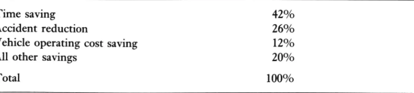
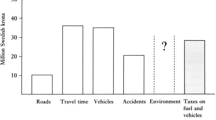
An illustration from the road transport sector of the total cost structure is given in gure 8.1. As is seen, for the transports produced on the state-owned
road network in Sweden, the total user costs of time, vehicles and traf c
accidents are some ten times greater than the total road expenditure, of which repair and maintenance make up three quarters. Road users also pay taxes on motor vehicles and fuel, which together outstrip total road expenditure by a factor of 4.
This structure is roughly representative of other transport systems in one
important respect, no matter whether based on rails, air or water, the user costs are dominant. Road transport systems stand out in two other respects.
Mi ll io n Sw ed ish kr on a
Government and Transport Infrastructure Pricing 193 50
40
30<9
20 10 lRoads Travel time Vehicles Accidents Environment Taxes on fuel and vehicles
Figure 8.1 Cost components in the total costs of road transport on the Swedish state-owned road network in 1990.
1 The high proportion of accident costs is unique. In view of the fact that the road transport volume constitutes some 80 per cent of total transport personal and freight it is apparent that (the lack of) road safety is of utmost concern.
2 The substantial excess of tax revenue over expenditure on roads is almost unheard of for the infrastructure of other modes of transport.
The economic justi cation for the overcharging of road users is that both the external costs of accidents (for sure) and the costs of noise and air pollution caused by road traf c (probably) are of an order of magnitude well above total road expenditure. The proven low elasticity of demand is probably a contributory explanation of why the strict earmarking of revenue from taxes on motor cars and fuel for road nance has been abandoned in most countries, with the notable exceptions of Japan and the USA.
The importance of being unimportant
The fact that the road owners total costs constitute a relatively small part of the total system costs is not the exception but the rule in the transport sector. The seaport and airport owners total costs are only a few per cent of the total costs of the terminal services in question, including inter alia the cost of ships
194 ]. O. ]ansson
laytime and the waiting time costs on the ground of airline passengers. In rail
transport systems, the total costs of the transport infrastructure services
con-cerned make up a higher proportion, on an aggregate level, than in any other transport systems; about 20 per cent would be a representative order of magni-tude. To beat this, one has to single out the road transport system of the inner areas of large cities, where the costs of the car parking facilities, owing to the high cost of land, will boost the transport infrastructure part of the total system costs.
In a transport chain of a number of links, it can be very important to be unimportant, to pursue the Hicksian pun. In the absence of good substitutes, it is possible to exploit the inelastic demand that follows from one s unimportance,
i.e. relative smallness, and the fact that each link in the chain is equally vital.
The generalized cost of different transport services corresponds roughly to the total system cost per unit of output. Given that the absolute values of the generalized cost elasticity for different modes of transport are to be found in the 1 2 band, with railway transport at the upper limit and road transport at the lower limit (compare the recent surveys of transport demand elasticities by
Oum et al., 1992, and Goodwin, 1992), it is possible to conclude that, looked at
as an aggregate, transport infrastructure services face price elasticities as low as from below 0.1 to 0.5 at most. So nancing transport infrastructure systems by user charges should be no great problem!
It must immediately be said that competition can make all the difference between complete inelasticity and almost in nite elasticity of demand. For example, when a new, better road between two points A and B is opened, its demand can have the characteristic logit shape , implying that below a certain price almost everybody chooses the better road, and above this price level only a few motorists with high values of time are willing to pay the price. If the old road is shut down, on the other hand, the demand for the new road may be come very inelastic. This simple fact is all-important for the nancial viability of toll roads.
8.3 COST AND OUTPUT RELATIONSHIPS
The re ected image of the transport production function approach is the fol lowing total cost categorization, where the costs of the transport infrastructure owner, i.e. the producer of transport infrastructure services, constitute just the
rst term:
TC : Tcprod + Tcuser + Tcext
Government und Transport Infrastructure Pricing 195 where TCprOd = f(X, Y, Q) is the total cost for the producer of transport infra-structure services as a function of facility design, physical conditions for the construction and the traf c volume; ACuser = g(X,Q/K ) is the average cost of users of transport infrastructure services as a function of facility design and the rate of capacity utilization; TCuser = g(X,Q/K )Q; TC?" = h(X,Q) is the total cost of the rest of society (apart from actors within the transport production system) as a function of facility design and the traf c volume; K = Ie(X) is the capacity of the facility as a function of facility design; X is the vector of facility design variables (width, curvature etc.); Y is the vector of physical conditions at the location of the facility (piece of transport infrastructure); Qis the output in terms of traf c volume; and _Q/K = (I) is the rate of capacity utilization.
It is practical to look at each of the main total cost components separately as long as the important interrelationship between the producer and user costs via the capacity K and/or the facility design variables X is borne in mind.
The reason for expressing the total user cost as a product of the average user cost per unit of traf c and the traf c volume is that the former factor is a basic entity for both cost and demand analysis. It is the real part of the generalized cost, perceived as the private marginal cost of an individual user, provided that his perception of his own travel/transport cost is realistic.
The section below looks at the short-run costs, which are dominated by the user costs, and the long-run producer costs in turn.
Shart run user costs
As indicated by writing the average user cost function as g(X,(I)), there are two
fundamental in uences on this cost that should be grasped: in the short run, when it can be assumed that facility design including its capacity is given, it is the rate of capacity utilization which is important, and in the long run, or rather in the planning stage of an investment, it is the effect on user costs of the design of the piece of transport infrastructure concerned that should be focused on. The special feature of capacity and quality jointness observed by Walters (1968), so far as roads are concerned, is a general characteristic of transport infrastructure. It is expressed here by making capacity K a function of the design vector X, as well as introducing X as a separate argument in the user cost function. For example, improving the alignment of a rail track increases the capacity and the running speed, given the capacity utilization. As a general rule it can be stated that when
£<O a_l<_>
8X
8X
Needless to say there are many other aspects of the relationship between facility design and transport infrastructure user costs. It is a wide and important
196 ]. O. jansson
area of engineering economy studies, which is well beyond the scope of this chapter.
Economists have been more concerned with the short-run relationship between the rate of capacity utilization (1) and user cost, presumably because it is of
direct relevance for optimal pricing of transport infrastructure services. Even in
this case engineering operational research, rather than econometric studies, is fundamental for our present knowledge.
The basic notion is that g as a function of (I) is more or less constant for low to moderate rates of capacity utilization, and rises gradually as the capacity limit of a particular facility is approached. In generalizing about the short-run user cost and output relationship a distinction between facilities for common use and departmentalized facilities is helpful. With common facilities like roads the rise in cost with an increasing rate of capacity utilization is caused by congestion. At departmentalized production plants congestion in the production process is avoided by definition. Instead, queuing before entering the production stage may occur. Congestion theory for road transport roads are the most important common transport infrastructure facilities and the character of congestion costs are well known and will not be taken up here. The user cost of occasional excess demand for departmentalized facilities like seaports, airports and parking facilities is not as well understood and will be briefly discussed.
In goods manufacturing a high rate of capacity utilization in the production stages is achieved by buffer stocks at both ends (of input material and finished goods, respectively). In the production of services, which cannot be stored, the target as regards the rate of capacity utilization has to be set at a much lower level. Otherwise the queuing time of customers will be intolerable.
Departmentalized facilities
seaport as an example
The general-purpose seaport supplies service to ships, cargo and land transport vehicles arriving more or less at random and making different demands on port resources. The short-term demand for port services will therefore vary one week all resources may be occupied and the ships will be waiting in the roads, the next week there may be no ships in the port at all. What is the correct trade-off between the two objectives of a high level of utilization of port facilities and a low likelihood of delays for ships?
A useful tool for tackling port optimization problems is provided by the theory of queuing: ships can be regarded as customers , while the service stations of conventional queuing models can be represented by the berths of a seaport. In fact, alongside telephone services, seaports constitute a major area for the application of queuing theory.
Government and Transport Infrastructure Pricing 197 time. It is the queuing time that depends critically on the rate of capacity utilization. The mean queuing time for customers (ships) arriving more or less randomly at a single-channel facility (a port section with one berth only) will rise quite steeply even at modest levels of utilization. If the customers capacity requirements differ signi cantly, i.e. if individual service times for loadingwand unloading a ship vary subs tantially,,-this tendency will be reinforced.
This can be illustrated, using elementary theory, on the basis of the following standard assumptions:
1 customers arrive at random, which means that the distribution of arrivals can be described by the Poisson probability distribution;
2 similarly, the duration of the service time is a random variable, tting the negative exponential probability distribution;
3 there is no upper limit to the length of the queue, i.e. customers are in-de nitely patient .
The expected queuing time in statistical equilibrium will then be 2
q = Jl = 5 2 (8.2)
1 As l (I)
where q is the expected queuing time per customer (days), A is the expected number of arrivals per day, s is the expected service time per customer (days) and (I) is the occupancy rate (= As).
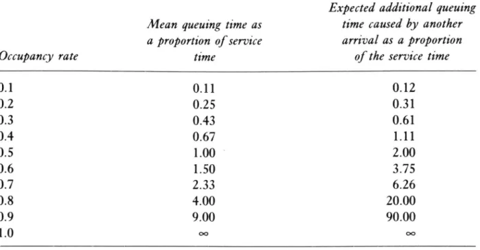
A characteristic of this model, as of many other more complicated queuing models, is that, given the occupancy rate, the mean queuing time q is propor-tional to the mean service time s. As can be seen, q moves towards in nity as (I) approaches unity. The sharp rise in the mean queuing time as the occupancy rate increases is shown in the middle column of table 8.1, which gives the ratio of q to 5 for different values of (I).
The root cause of the queuing that occurs is, of course, the variability of A and 5. The laytime of similar ships varies because a great many more or less random factors signi cantly affect the actual value of the service time. Such factors include the weather and stoppages due to breakdown of handling or other equipment. In addition, the type and size of ships and the type of cargo can vary a lot. What difference does it make if the variability of s can be reduced? The Pollaczek Khintchine formula provides a general answer to the question of how the mean queuing time is affected by the distribution of service time. It states that for any arbitrary distribution of s it is possible to express the steady-state mean queuing time q as a function of the arrival rate A, the mean service time 5 and the variance var(s) of the service time distribution:
2
q : A[s + var(s)] (8.3)
198 ]. O. ]ansson
Table 8.1 Queuing time in the single-stage single-channel model
Expected additional queuing Mean queuing time as time caused by another
a proportion ofservice arrival as a proportion
Occupancy rate time of the service time 0.1 0.1 1 0.12 0.2 0.25 0.31 0.3 0.43 0.61 0.4 0.67 1.1 1 0.5 1.00 2.00 0.6 1.50 3.75 0.7 2.33 6.26 0.8 4.00 20.00 0.9 9.00 90.00 1.0 oo oo
In the case of a negative exponential distribution of s, the variance is sz. It is easily checked that the previous expression (8.2) for the mean queuing time is obtained by inserting this for var(s) in (8.3). In the case of constant service time, the variance of s is zero and the general formula gives
4 = i (I)
2 1 (I)(8.4)
The elimination of service time variability will, ceteris paribus, reduce the mean queuing time by half.
It is clear from expression (8.3) above that, given the occupancy rate, the mean queuing time is proportional to the sum of the service time and its relative variance (5 + var(s)/s). Consequently, to reduce the queuing time it is as im-portant to achieve a reduction in the variability of the service time as it is to achieve a reduction in the mean service time itself. In the case of seaport operations this means that the expected queuing time may be reduced either by increasing the handling speed or by making each call by the ships more homogeneous, e.g. by specializing in serving a particular type of ship or cargo.
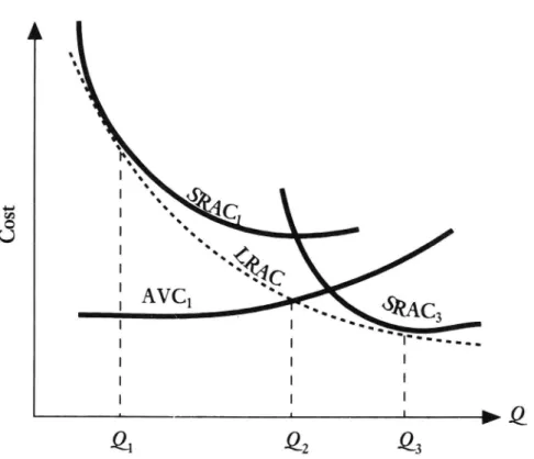
Long run producer costs
Cross-section cost studies of transport infrastructure have a special interest because there is ample opportunity to trace out the entire long-run relationship between cost and output. The whole range of the general L shaped average cost
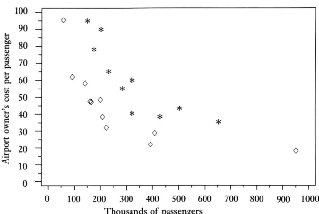
Government and Transport Infrastructure Pricing 199 100 90 80 70 60 50 40 30 20 10 Ai rp or t ow ne r s co st pe rpa ss en ge r i l i l l l i l l l i l i l l l l l i ll T T I ' T ' I ' I ' I ' 1 # I ' I ' I ' I 0 100 200 300 400 500 600 700 800 900 1000 Thousands of passengers
Figure 8.2 Airport cost per passenger against passenger volume.
Source: SOU, 1990
curve will be represented among the observations. In manufacturing industries, the average costs of all plants and/or rms of a particular industry making easily transportable goods should be more or less on the same level; a high-cost plant or rm could not survive where all plants in the industry serve the same national or even global market. Individual roads, on the other hand, are natural local monopolies. The fact that a particular motorway produces road services at a fth of the cost per vehicle-kilometre of a small road between two villages in a different part of the country is of no consequence for the viability of the latter.
Small scale diseconomies
The main proposition is simply that very marked small scale diseconomies are revealed by the empirical evidence, while it is more dif cult to say what will happen at the other end of the scale.
The airport owner s total cost per passenger for the 24 primary airports in Sweden illustrates well the magnitude of small-scale diseconomies that is typical. The impression given by gure 8.2 is a little distorted by a systematic cost difference between two categories of airport partly military and/or municipality owned versus state-owned. By including an appropriate dummy variable in the regression of average airport cost on passenger volume the main message is very
200 ]. O. ]ansson
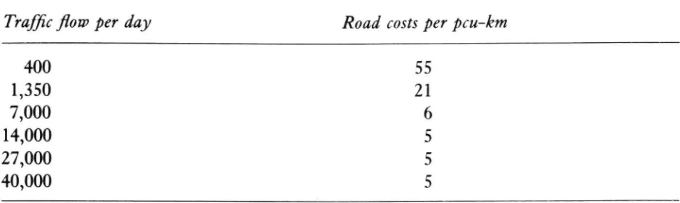
Table 8.2 Road capital and running costs per passenger car-unit(pcu) kilometre for different least-cost road designs
Trafic ow per day Road costs per peu lem
400
55
1,350
2
7,000
14,000
27,000
40,000
( 1 1 m e Source: Jansson, 1984clear: airports serving passenger volumes in the range lO0,000 200,000 per year are some ve times more costly than airports serving 1 million passengers.
By international standards 1 million passengers per year is not a large volume. There are three Swedish airports handling traf c volumes exceeding that limit; they did not t into the diagram of gure 8.2, especially not Arlanda, the biggest, which handles 15 times more passengers than the biggest airport rep resented in the diagram. Big airports have a more diversified line of products than small airports, which is why it is a little more dif cult to calculate a single, comparable unit cost; it seems, however, that all three outliers are at the cost level of the two airports with the lowest cost in the diagram.
A similar cost picture for British airports is given by Doganis and Thompson (1975)
When it comes to roads the highway engineering manuals point in the same direction: very marked diseconomies of small-scale-operation prevail, but the scale economies seem to be largely exhausted in the traf c volume range where motorway standards are justi ed. Since topography and the condition of the soil can differ greatly, the variability in construction costs is quite signi cant. The gures in table 8.2 are rough averages: within each class of road, capital costs that are twice as high per kilometre or only half the value given are not rare.
There is no empirical evidence of rail track costs taken separately. Sweden so far is the only country in the world with a formal separate rail track adminis-tration (*Banverket ). It has not existed long enough to produce reliable gures
of the cost of rail track services with respect to traf c volume. There is no reason to doubt that the cost picture is much the same as for roads. The
question of economies of scale in rail transport (rail track and train) services was once a hotly debated issue, until it was made clear that one has to distinguish
Government and Transport Infrastructure Pricing 201 rm size economies and economies of traffic density. Why were twig and branch lines closed down when the Railways Administration tried to improve its nancial position? Obviously it was because costs per unit of traf c are typically many times higher there than on trunk lines, in spite of a high sunk
cost portion of the capacity costs. Harris (1977) pointed out the irrelevance of
the question of rm size economies for the issue of line discontinuation, and
showed that signi cant economies of traf c density exist in the US rail freight
industry. The average costs comprise both track costs and freight train costs in that case. It seems, however, that more than half of the sharp cost decline is due to strong small-scale diseconomies in the capital and maintenance costs of the rail track.
When it comes to departmentalized facilities, multichannel queuing theory provides good insight into the root cause of the very marked small-scale diseconomies of this kind of service production plant.
Suppose that the seaport model discussed above consists of n identical berths rather than just a single one. Under the same conditions as in the previous model, the standard multichannel queuing model can be used for predicting how far queuing time depends on the rate of capacity utilization. Since this model is mathematically more involved, it will be helpful to derive the steady-state mean queuing time in two steps.
Let p be the probability that an arrival will nd all channels occupied. The mean queuing time can then be written as
S
4 = _!)
(8-5)
n(1 (I))
The occupancy rate (I) is now As/n. The left-hand factor represents the ex-pected queuing time for those customers who actually meet with a delay, while 1) is the probability that a delay occurs. This probability is a function of n and (I), but is independent of 5. This means that the proportionality between q and 5, which applies in the corresponding single channel model, is retained in this multichannel model.
The in uence on the queuing time of the number of service stations origin ates from both factors in (8.5). Given the occupancy rate, the value of the left hand factor is inversely proportional to n. This is an interesting relationship. If the occupancy rate remains constant when demand increases, i.e. the number of service stations grows in proportion to the demand for service, the total queuing time will be equal to a constant multiplied by p. And given the occupancy rate, 1) decreases continuously as n increases. This is a well-established fact of
queu-ing theory (see, for example, Saaty, 1961). From numerical simulations it is
clear that the combined effect of these two factors makes the advantages of multichannel service facilities truly remarkable. The total queuing time decreases when demand and capacity increase at the same rate.
202 ]. O. jansson
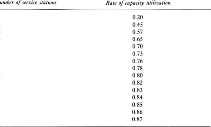
Table 8.3 Possible rates of capacity utilization for maintaining a given quality of service
Number ofservice stations Rate of capacity utilization
1 0.20 2 0.45 3 0.57 4 0.65 5 0.70 6 0.73 7 0.76 8 0.78 9 0.80 10 0.82 11 0.83 12 0.84 13 0.85 14 0.86 15 0.87
Another expression for the same relation is given by the figures in table 8.3. Holding the quality of service constant, i.e. given the expected queuing time per arrival at a level of, say, a fth of the service time, the rates of capacity utilization possible for facilities of successively more service stations are as shown.
Finally it can be mentioned that the economies of number can be realized either in the form of lower queuing costs, lower capacity costs per customer, or a combination of both. It can be shown that the occupancy rate will increase steadily along the expansion path , while the mean queuing time will decrease. This means that both the capacity cost and the queuing cost per unit of throughput will fall as throughput increases, provided that an optimal factor combination is chosen.
Are the plant-size economies boundless?
It is interesting to see that the economies of number of service stations are almost exhausted for n in the range 10 15. This is a feature which reappears in many other cases, also of common facilities. The old idea that there is a limit to everything may apply also to transport infrastructure facility size economies. Large scale diseconomies may set in sooner or later to balance and eventually offset the kind of economies which have been focused on here and which, no
Government and Transport Infrastructure Pricing 203 doubt, initially are very prominent indeed. There is no space to go deeply into the question of whether an L-shape or a U-shape is most characteristic of the long run average cost of transport infrastructure service production. A modest example is given in gure 8.3 of an empirical result pointing to the possibility that diseconomies of density of demand may in fact exist in the area of transport infrastructure service production.
A cross-section study of the total costs of staff for sale of tickets including seat reservation, information etc. at railway stations in Sweden and the number of tickets sold was made as part of a project concerning railway transport pricing (jansson et al., 1992). The data can be divided into one large group of small and medium-sized stations and a small group of large stations. In the former group the total cost and output relationship has the expected degressive shape gure 8.3(b). When both groups are considered, the remarkable result is that the textbook cubic relationship appears: increasing returns are succeeded by decreasing returns. It should be pointed out, however, that the uncertainty is much greater in the interval where observations are few.
At the system level, there is at least one important example of decreasing returns in the production of road services. For radial road transport in big cities there is a long-run capacity limit that shows itself in increasing costs of various kinds as more and more of the extremely scarce space is taken up by roads and parking facilities. In mega-cities like Tokyo, New York and London the car share in the market for central city commuter trips does not exceed 10 per cent. The passenger ow capacity of car traf c per metre of track width is relatively low, which means that elevated expressways have to be constructed if the market share of car traf c on radial routes of urban areas is to be substantially increased, and this is obviously an increasingly costly option, if it is an option at all in view of the environmental harm.
8.4 OPTIMAL PRICING
To the man in the street, the rationale for charging for transport infrastructure services is that roads etc. cost a lot to provide and maintain. Since Dupuit (1844), transport economists have had the hardly enviable task of explaining that this is not so: charges for transport infrastructure services should ensure an ef cient use of facilities, which means that a great many pieces of transport infrastructure, in addition to Dupuit s bridge, should be free. The man in the street is then likely to follow up his argument by the rhetorical question: who should nance the building and maintenance of the bridge, if the use of it is free?
One reasonable answer is that the total road network contains many links, in particular in urban areas where demand exceeds supply by far, and these links
18,000 fc? _ ::o _.
£2
__
å 12,000
as
:
g __ U &: __ ä 6000 73 - I 5 _ F _ 0 _ ,I
I
I
I
I
I
0 300,000 600,000 900,000 1,200,000 1,500,000 (a) Number of tickets sold6000 f; _ :: D _|
3
_
% 4000
-zz
:
-% _ & - I & 2000 -TG 1 E' __ F . O _ ,
I
I
I
I
I
0 100,000 200,000 300,000 400,000(b) Number of tickets sold
Figure 8.3 Relationship between total staff cost and the number of tickets sold: (a) for all SJ stations; (b) for S] stations where sales are below 450,000 tickets per year.
Government ana' Transport Infrastructure Pricing 205 should have prices that cover their total costs many times over: spatial cross-subsidization between markets of high and low density of demand should be a typical pattern in transport infrastructure systems if ef ciency is a principal objective.
Even a normally very busy road is sometimes almost empty. Peak load pricing is strongly required for many transport infrastructure services, and so cross-subsidization in time is equally characteristic of an ef cient price struc ture in the transport infrastructure sector. This pattern is clearly in sharp contrast to the present uniformity in time and space of prices for transport infrastructure services.
The pricing relevant cost of transport
infrastructure services
For the existing pieces of service-producing transport infrastructure the facility design, including capacity, is xed for a long time onwards. Now the best use will have to be made of the resources available. For any given piece of transport infrastructure the objective should be for each period of time to maximize the sum of the consumers surplus and the producer s surplus minus the costs of negative externalities falling on the rest of society. The total costs as written in equation (8.1) represent the cost side in the following net social bene t maximization. The gross bene t to users is represented by the integral of the applicable marginal utility (MU) function.
MU = U(Q)
(8.6)
Q
consumers surplus = L) U(Q)dQ
(P + ACUS")Q
The gross bene t is de ned not to include the user costs of time and other real efforts to come into possession of the service in question: to arrive at the consumers surplus, both the price P paid and the user cost ACuser have to be deducted from the gross benefit.
producer s surplus : pg _ TCprod
total external cost : TCext
Adding up these three items gives the total to be maximized:
Q
net social bene t (NSB) = jo U(Q)dQ _ Q Acuser _ Tcpmd _ Tcext
Specifying the cost functions according to equation (8.1), but taking into account that the facility design variables are xed and therefore can be ignored, yields this nal form of the maximand:
206 ]. O. jansson
Q
NSB = [0 U(.Q)dQ g(Q) Q f(Q) MQ)
(8.7)
The sum of price P and the average user cost ACuser is customarily called the generalized cost (GC):
GC : P + g(Q) (8.8)
An equilibrium condition that has to be observed is that GC equals the mar ginal utility:
P + g(Q) = U(Q)
(8-9)
Now, taking the derivative of NSB with respect to quantity Qand setting it equal to zero gives the following rst-order condition for a maximum:
ÖNSB
Ög
=U(Q)
g(Q ___ =O
(8-10)
ÖQ
ÖQ
GQ
ÖQ
Substituting P + g(Q) for U(Q) from (8.9) gives the nal result:
P = if + Qå + Eh : MCprod + QM + MCm (8.11)
ÖQ
ÖQ
ÖQ
GQ
Unsurprisingly the above ends up with the well-known postulate that, for maximum net social bene t of the existing pieces of transport infrastructure, a necessary condition is that price is set equal to the sum of the short run marginal cost of the producer of transport infrastructure services, the cost imposed on fellow users and the cost imposed on outsiders by an additional user of the transport infrastructure facility concerned.
The rst item consists mainly of use-dependent wear and tear and is nor-mally rather small. The second item is usually called the congestion cost com ponent . This and the third item, which contains a variety of negative extemalities, are the major components in the pricing-relevant cost. Now its content will be looked at more closely for common facilities as well as departmentalized facilities.
Common facilities
With a common facility like a road, the users interference with each other takes two related forms a reduction in speed to avoid collisions when traf c density goes up and (multi )vehicle accidents that occur in spite of speed moderation. Some excellent work on road pricing theory and problems of application exist for which the speed ow relationship forms the basis. Mention can be made of
Government and Transport Infrastructure Pricing 207 and a recent survey by Goodwin and Jones (1989; as well as Jansson et al., 1990). Here another somewhat neglected aspect is taken up. Total accident cost
in road transport is approximately half the total cost of travel time, and so
potentially the relationship between traf c accidents and the intensity of traf c
is very important.
Empirical studies with a view to establishing a functional relationship be tween traf c accidents and probable determinants such as traf c ow are very dif cult because of the fortunate fact that accidents are rare occurrences. In a cross-section study where traf c on different roads constitute the observations, the observation period has to be rather long in order to arrive at a reasonably representative number of accidents in each particular case (road). And during that long observation period, explanatory variables such as weather conditions, the state of the road, the composition of traf c as well as the traf c ow do not stay constant. A lot of averaging is inevitable, which greatly reduces the accur-acy of the data.
So far the weight of evidence speaks for a constant risk for accidents per unit of traf c with respect to traf c ow, in a range from rather high traf c density to free ow, all other things remaining equal.
The constancy hypothesis is the somewhat shaky basis for the current treat-ment of accident costs in calculations of optimal road user charges, which in the briefest possible summary is as follows.
The expected accident cost per car-kilometre is bc, where b is the constant (traf c ow invariate) risk and [ is the expected cost per accident. The latter
unit cost is divided into three main components: 6 = 61 + 62 + 63 where cl is the
human warm blooded costs of death and injury (for principles of valuation of these costs see chapter 5) and cz and 63 represent the external cold-blooded re-source costs, of which 62 is the expected value of the difference between future production and consumption of victims of an accident and £3 is the cost of hospital
treatment etc.
The basic hypothesis is, as mentioned above, that an additional unit of traffic does not increase the accident risk for the existing traffic. Since the idea of optimal road user charges is to make road users aware also of the external costs of road use to the rest of society, the accident cost component in the charge is normally obtained by taking b(c;_ + 63) minus the possible part of the total traffic insurance premium intended to cover some external costs.
This principle of calculating the pricing-relevant accident cost seems in-complete when it is taken into account that different categories of road users constitute very different threats to each other. The main difference is between unprotected road users, i.e. pedestrians, cyclists and motorcyclists, and those travelling in cars and buses. It must be borne in mind that the accident risk per
208 ]. O. jansson
the accident risk of unprotected road users, bn. Therefore there is also a dif-ference between private and social costs as regards the human cost component; the car user is facing a private human cost equal to bla,, but the change for car use should also include the expected human cost of death and injury suffered by unprotected road users, equal to bnc].
In cost bene t analyses of road investments in many countries the human costs of traf c accidents play an important role on the bene t side. For ef ciency in resource allocation, human costs should play a fully congruous role in the road user charges; lives of unprotected road users will be saved by car traf c reduction. If the human cost values applied by national road administrations for investment appraisals were also applied for the calculation of road user charges, an appreciable rise of these charges in urban areas would be indicated in many cases, even on uncongested roads (for a further discussion see OECD, 1985).
Departmentalized facilities I: patient customers
The queuing model outlined in the previous section gives one simple example of how the pricing relevant cost could be calculated in a situation where occa sional excess demand leads to an actual waiting line. The optimal price should be equal to the expected additional time cost caused by another customer to the rest of the customers. For example, at an occupancy rate of 0.6 this cost is (3.75 l.50)sm = 2.250?) in the single-channel case illustrated in table 8.1, where s is expected service time and m is the value of waiting time. As seen, the pricing relevant cost rises steeply with occupancy rate. For (I) = 0.9 it is as high as 813117.
In practice it can be rather dif cult to calculate the applicable queuing cost function (cf. Jansson and Shneerson, 1982), but it is even more dif cult to estimate accurately the matching demand function. Some trial and error is necessary before the right solution can be found, i.-e. before the price is found which equals the pricing relevant expected cost.
In this case, as in many other cases in transport, there is the problem of perceived versus actual cost. The price theory presumes that each customer knows what to expect both as to queuing time and as to service time. The price is just motivated by the delay caused to others. Suppose customers systematically under or over-estimate the time requirement, either the mean queuing time or mean service time or both. Should that be re ected in the price? There are arguments both for and against. One can argue that the marginal time cost should be equal to the sum of price and the perceived average time cost rather than the sum of price and the actual average time cost. On the other hand, it is somewhat unsatisfactory to burden customers twice when actual costs are under-estimated, or to fail to include the whole cost of delay caused to others in the price when actual costs are over-estimated.
Government and Transport Infrastructure Pricing 209
Departmentalized facilities II: impatient customers
The queuing model case above is the simple case. Much greater dif culty in monetizing the user costs of excess demand arises in cases where these costs assume the shape of frustration of not attaining possession of service at the facility concerned, because queuing would be out of the question.
This case may in turn be divided into
1 the case where customers go to another facility for the same service, and 2 the case where the excess demand cannot be satis ed anywhere but simply
drops out (for the time being).
Urban parking can provide good examples of both cases: if a particular down-town parking garage aimed at is fully occupied, one looks for another, or knowing from experience that on, say, Saturday night it is very dif cult to nd parking space reasonably close to the theatre district, one refrains from going downtown for the theatre altogether.
The latter case and the previous queuing model with completely patient customers are two polar cases. All sorts of in-between cases exist. The common characteristic is that the pricing-relevant cost occurs as a result of excess demand before the proper production starts. In each particular case, a suitable represen-tation of the cost of occasional excess demand seldom comes easy. One should not aim at perfection . In practice peak-load pricing of services provided at departmentalized transport infrastructure facilities, if it exists at all, is rough and ready. The important thing is to understand the nature of user costs of excess demand and, second, to try to get a quantitative idea of its relationship with the mean rate of capacity utilization. It should perhaps also be said that one must not be misled by simplistic deterministic models, where 100 per cent capacity utilization is a natural target. Last but not least, good Fingerspitzengeju'hl (intuitive feeling) is required to devise an ef cient price structure by time period.
Pricing of transport infrastructure services versus
pricing of transport infrastructure gooa's :
par/eing pricing as an example
An alternative way of looking at the product so far called transport infrastruc-ture services is to View it as very-short term renting of space of a transport infrastructure facility, where the rst come, rst served principle is applied. It is then interesting to note that this transaction form is one end-point of a continuum, where the other end-point is to purchase a whole piece of transport
2 10 ]. O. jansson
infrastructure for one s own exclusive use. The latter option is quite frequently
chosen by big users as regards departmentalized facilities. A middle form is the renting of a piece of transport infrastructure on a long-term basis, e.g. a berth
with supplementary transit storage facilities in a seaport. Liner shipping com-panies often choose this transaction form to avoid the risk of queuing time. In the case of what is usually regarded as common facilities, buying or renting a whole piece is more rare, but strictly private roads and private sidings com-plementing the national rail network exist. From a price theoretical point of
view this difference in transaction form is really fundamental: it changes the
object of pricing from non-storable services to goods, and it can change the market form from one extreme of (local) monopoly to the other extreme of almost pure competition.
The parking market
In the parking market the whole continuum of transaction forms is well repre sented. Since parking is an important transport infrastructure service in its own right, it is worthwhile to look closer at parking in urban areas.
For a car commuter working in the central business district of a million-city the parking cost is the dominant component in the daily travel cost, pro-vided that he has to pay the full market price for a parking space, which is rare for various reasons. Then the daily parking cost can be anything from $6 upwards depending on city size, whereas the private car operating cost of the journey itself is normally below $6. In a city like Stockholm the cost of renting a parking space on a monthly basis is about $6 10 per day in the central
business district. In central Tokyo, for instance, or on lower Manhattan it is
many times more.
Looking at the parking market from the demand side, a useful distinction is between parking at the base and parking away from the base . Like its owner, every car has a home, or base , where the car is kept at night time etc. The characteristics of the demand for base parking are (i) that each parking period is fairly long term and (ii) that it occurs frequently and at the same place.
When the car is used for various trips to destinations away from the base
to shops, to visit customers, to do different errands short term occasional
parking in many different places is needed.
In the base-parking market segment, parkers typically own or long-term hire parking space, and in the other market segment parkers pay per hour of park-ing space occupation. It is the same market segmentation as in the market for accommodation with owner-user apartments at one end and hotel rooms at the other. The interesting additional fact, however, is that whereas the price of a hotel room per night is many times higher than the rent of a comparable at, this rational price ratio is often upside down in the parking market.
Government and Transport Infrastructure Pricing 211
Occasional short-term parking on-street and base-parking
off-street
a natural division of the parking market
Optimal on-street parking pricing is a fairly complex matter when it comes to the detailed structure of the charges by time period. A basic feature, all the same, is that the average level of charges should not deviate too much from the value of the land used. If the average level of on street parking charges is much
higher, more curbstone spaces should be provided, and if it is much lower,
better use of some of the existing curbstone parking space could probably be found.
Bearing this in mind, the appropriate relative prices of on-street and off street parking can be considered: normally, on-street parking should be sub stantially more expensive than off-street parking because
I the former is provided on a per hour basis, whereas garage space etc. can be rented on a monthly basis; and
2 the cost of the land taken up can be distributed between several floors in the multi storey parking garages typical of central cities.
With such a price structure, which in fact is reversed in many cities in the world, a rational division of short term and long-term parking would arise: long-term parkers could simply not afford to park in the streets, where practically only short term parkers would be found.
8.5 WILL OPTIMAL TRANSPORT
INFRASTRUCTURE CHARGES PAY FOR
THE FACILITIESP
The normal procedure in price theory when the question of the nancial result of optimal pricing is taken up is to explore whether or not economies of scale apply. When both short-run and long run ef ciency conditions are ful lled, a well known implication is that the ratio of optimal price to the average total cost equals the inverse of the scale elasticity of the production function concerned. Economies of scale imply a nancial de cit and diseconomies of scale a surplus as a result of optimal pricing.
When it comes to optimal pricing of transport infrastructure services, the scale elasticity of the production function plays a similar critical role for the nancial result. However, there is an additional condition which tends to make the nancial result of optimal pricing much more sensitive to deviations from constant returns to scale. This will be explained in what follows.
212 ]. O. ]cmsson
Congestion tolls as ot contribution to tmc/e costs,
or 'quasi rent'
The discussion will be limited to congestion tolls or the equivalent type of charge for regulating capacity utilization. The pricing-relevant cost also in cludes an item MCem to account for the signi cant negative effects external to the traf c: noise, air pollution and certain consequences of traf c accidents are the most important in this category. These components in the optimal price of transport infrastructure services cannot be viewed as contributing to covering the facility capital costs. If charges with a purpose of internalizing the costs of negative externalities such as exhaust fumes were to be earmarked for something, it should be for compensation to those who suffer from the negative externalities. Even if transport vehicles eventually become silent, clean and safe, the basic reason for charging for their use of roads etc. will remain where and when various pieces of transport infrastructure are scarce resources. So the basic question is whether optimal congestion tolls would pay for the facility concerned. It turns out that the form of organization of transport has an interesting role to play in this connection. A number of cases can be distinguished. The rst case below is imaginary but instructive as a starting-point.
Case (a): Fully integrated road transport system
Imagine a road transport concern where the road owner is also the seller of transport services: the unit of output is a standard truckload kilometre. It can be assumed either that the road owner also owns all the trucks or that he acts as a forwarding agent and just hires truck inputs on behalf of shippers. The objective is assumed to be net social bene t maximization.
In gure 8.4 the average variable cost (AVC) represents the costs of the truck inputs per truckload-kilometre. The fact that the AVC is gradually rising is due to the given capacity of the road network. Since the road owner controls all truck movements, he calculates the short run marginal cost (SRMC) by taking the derivative of the total truck transport cost function with respect to total output of truckload-kilometres.
There is no allocative need for a separate road track charge: the congestion costs are internal to the transport concern. The difference between SRMC and AVC constitutes the contribution margin , C in the diagram of gure 8.4, in the price P for the transport services, i.e. the nancial contribution to wards covering the track costs. In microeconomics textbooks this is often called
quasi rent .
It should be assumed that operations take place at the expansion path : the least-cost solution, including the track costs, is found for each actual level of
Government and Transport Infrastructure Pricing 213
Å LRAC
s SRAC Demand '. SRMC 0) s. ,.a
__
a:
P """"""""""""""" {. AFC
Ci
AVC
: > Q Output (truckload-kilometres) Figure 8.4 Ideal output Q and price P for transport services.output. It is then helpful to introduce the scale elasticity E of the truck trans port production function: E = 1 means that constant returns to scale apply, E < 1 means decreasing returns to scale apply and E > 1 means increasing returns to scale apply. As P is set equal to SRMC the following holds:
l _
SRMC
(8.12)
E AVC + AFC
Where AFC stands for the average xed cost in the short run, which corre-sponds to the road track cost per truckload-kilometre in the present case. From (8.12) it can be seen that the nancial result of the whole concern, measured by the ratio of total revenue to total costs, is equal to the inverse of the scale elasticity E.
This is, of course, elementary and very well know. The question focused on here is how the contribution margin is related to the road track costs under different conditions as to returns to scale. The main point should be intuitively clear, since the contribution margin is a residual by nature: in the rst place the short run variable factors of production are fully remunerated (this cost cor responds to AVC). The contribution to the short-run xed costs will be what is left of total revenue after that remuneration is paid out.
The ratio of the contribution margin C per unit of output to the track cost is written
214 ].0. jansson
C _ MC AVC (8.13)
AFC AFC
Combining equations (8.12) and (8.13) gives the following result:
(: _ [(AVC
AFC)/E] AVC _ _1_ + AVC l _
(814)
AFC
AFC
"" E
AFC E
'
When constant returns to scale apply (E = 1), the last term on the right hand side of (8.14) is zero and, as expected, the contribution margin is just sufficient to cover the track costs. When E deviates from unity, the effect on the C/AFC ratio is strengthened by this additional term: when increasing returns apply, the contribution margin falls short of track costs to a larger degree than is indicated by the inverse of E, and conversely when decreasing returns apply the differ-ence between the optimal price and the average truck transport cost will be still higher than is indicated by the inverse value of E.
From the point of view of the whole road transport concern, however, the ratio of the contribution margin to the track cost is just an accounting relationship. The financial result of the concern depends on E, exactly as the textbook has it. In the next, real world, case this will appear to be different.
Case (b): One road owner, many truck transport operators
In reality the road owner has no direct co ordinating power over truck traf c but has to rely on incentives such as congestion charges. It can still be assumed that AVC of the previous model corresponds to the remuneration per truckload kilometre to truck owners. The only difference in this case is that what previously could be regarded as a track cost contribution margin in the price of transport services is now an actual road user charge. The financial result for the whole road transport sector will be the same as in the previous case, assuming, of course, that optimal congestion tolls are levied.In the present case, however, the trucking companies and the road authority make separate nancial accounts. The nancial result of the road authority corresponds to the accounting ratio of the contribution margin to the track cost in the previous case. The fact that this ratio can take values in a much wider range than follows from normal deviations from unity of E is a matter of some concern.
The cost picture is exactly the same as before except for the following changes in designation:
AFC => ACperd = average road service producer cost AVC => ACuser = average road user cost
Government and Transport Infrastructure Pricing 215
Table 8.4 The nancial result for the owner of the transport infrastructure of optimal pricing C/ACpmd for different values of the scale elasticity E and the ratio of
Acuser tO ACprod Scale elasticity E ACM/AGW! 0.8 0.9 1 1.1 1.2 0 1.25 1.11 1 0.91 0.83 1 1.50 1.22 1 0.83 0.66 2 1.75 1.33 1 0.72 0.49 3 2.00 1.44 1 0.64 0.32 4 2.25 1.55 l 0.55 0.15 5 2.50 1.66 1 0.46 0.00
Expression (8.14) for the ratio of the contribution margin to the fixed capital cost is renamed the ratio of the congestion toll to the track cost and conse-quently is rewritten as
C : l. + AC
_l 1
(8.15)
ACprOd E ACprOd E
Baa news about the nancial result of optimal
congestion charges
The rst observation is that the ratio AC m/ACprOd normally takes relatively high values. In the total costs of a transport system be it road transport, air trans port or sea transport the transport infrastructure costs are a relatively minor part. In personal transport in particular, ACuser is typically many times greater
than ACprOd because the time and effort of persons are dominant items. This
gives the above formula a markedly high-geared character: as soon as E is different from unity, the last term becomes operative, and when ACuser/ACprOd has a high value the nancial result, C/ACpmd, will deviate widely from the value of 1/E. In table 8.4 this is illustrated by some examples where the scale elasti-city is varied around unity and where the ratio of user cost to producer cost of transport infrastructure services is increased from 0 to 5.It is interesting to note, for example, that in interurban and rural road transport the ACuseVACpmd ratio is at least 5. The scale elasticity is not constant with respect to traf c volume; in the range 400 40,000 vehicles per day it is about 1.2, on average, according to highway engineering cost studies (Jansson,
216 ]. O. ]ansson
By pointing out the jointness of road capacity and quality (see section 8.3), Walters (1968) argued that roads approximate public goods in a wide initial range of traf c volume. A simpler and more general explanation is apparently to hand, which also expounds the dramatic change in optimal charges from zero to a level of twice the track costs or more. It does not contradict Walters original idea. However, labour saving capital investment is not special for road transport. In many industries the larger plants often have a markedly labour-saving potential. The special feature about road transport is that the capital services are disintegrated from the labour and charged for separately.
The problem is that zero charges for public goods, for which excludability is technically possible, are not acceptable for reasons other than allocative ef ciency. At the other end of the scale it is easily imagined that road pricing for central city bound traf c that brings in revenue that covers radial road investment costs many times over is quite consistent with ef ciency conditions. However, now that the technique for charging urban traf c exists, the lasting dif culties of getting acceptance for urban road pricing bear witness to the opposition to the idea that the motorists of a particular city should pay two or three times more than is spent on the roads of the city in the form of congestion tolls on top of the fuel tax.
A similar impasse exists as far as the congestion problems of big city airports (and airways) are concerned: ef cient congestion tolls would most probably cover airport costs many times over, but no one seems to have the determination and/or voter support to introduce them.
In previous literature exploring the relationship between short-run and long-run costs of road transport (notably Mohring and Harwitz, 1962; Mohring 1976; Small et al., 1989), the point that has been emphasized is that optimal congestion tolls just cover the total road investment costs in the case of constant returns to scale. This was presented as good news, and it is no doubt a soothing possibility for the con ict averse, but it is representative neither of rural and interurban roads nor of urban roads.
Other modes of transport should also be considered in this connection.
Rail track charges, airport and seaport pricing
Case (c): Fully integrated rail transport system
The railways have until recently been the only mode of transport where the fully integrated form of organization of case (a) exists. It is true that this situation is gradually changing, as has already happened in Sweden and will happen in countries such as Britain and the Netherlands. Leaving these more recent developments out of the discussion for the moment, the ratio of the contribution margin in the fares to the rail track cost obeys the same formula
Government and Transport Infrastructure Pricing 217 (8.14) as was deduced earlier. The interpretation of E and AVC respectively, however, is different when a public transport undertaking is the track user. The Mohring effect , i.e. that additional passengers lead to positive external effects on the original passengers via a rise in the frequency of service,\makes a sub stantial difference compared with the hypothetical case (a) where full-load transport for hire makes up the system output. It is necessary either to take this effect into account or to extend the system de nition to comprise complete door-to-door transport chains. In the latter case the relevant scale elasticity E should be calculated on the basis of a production function in which the trips to and from railway stations and the frequency delays (cf. Panzar, 1979) of train passengers are treated as inputs on a par with rail track and trains. This system extension will tend to make economies of scale (or, better, economies of density of demand) more pronounced. Even more important is that the ratio AVC/ AFC will rise very considerably when passenger access and waiting time and effort are included together with the costs of the train operator.
While not going deeper into this matter it is worth discussing some organ izational variants of the main case of a fully integrated railway transport system.
Case (d): The Swedish model of one rail track owner and
a separate main line train operator
In the present Swedish case where only one train operator (SJ) uses the main rail network, the separate track owner (Banverket) should not charge any con-gestion tolls because the concon-gestion costs are already internalized in SJ s accounts. SJ can and should keep the quasi rent for itself. To require S] to pass it on to Banverket would lead to a misallocation of resources. It would mean that S] pays for congestion twice, both in the form of delays, which it is entirely aware of, and in the form of rail track charges. This would result in too little congestion in the rail network, so to speak, i.e. too low a rate of capacity utilization.
From the point of view of Banverket, the nancial situation looks rather odd. No matter whether constant, decreasing or increasing returns to scale prevail in the railway transport system, S] should make no contribution to the track costs of Banverket; only traf c dependent rail track wear and tear should make up the rail track charges. Banverket is and should be a subsidized enterprise. The total corresponding nancial burden on the central government would not, of course, become lighter by a merger of Banverket and SJ, i.e. a return to the old form of organization.
Looking at S], the corollary may seem to be that the government should require that a substantial pro t is made even when the goal is net social bene t
maximization, since all the quasi rent stays with S]. This is not necessarily the
218 ]. O. jansson
An additional point is that the nancial requirements on S] should be differ entiated. On some lines, where rail track services are next to public goods, a de cit for S] is consistent With net social bene t maximization. On other lines, the opposite should apply.
Case (e): One transport infrastructure owner and a few
transport infrastructure users/transport operators
A basic idea of the Swedish separation of track and trains is that, eventually, competition on the rails should be possible. The road transport system and rail transport system would then be organizationally more or less equal. Congestion charges on trains could be justi ed provided that there are a fairly large number of independent train operators (on the same line, which seems rather unlikely). The latter will probably argue that they can co ordinate timetables etc. by negotiation without the stimulus of rail track congestion charges.
That hypothetical situation resembles the present state of affairs of congested airports, where peak-load pricing is long overdue. Airlines naturally view this as just another unwanted cost increase. It may well be true that the allocation of slots between airlines can be managed without resort to the price mechanism. The main economic problem, however, is that airlines individually and/or collectively fail to establish the peak/off peak differentials in the fare structure which would be forced upon them, as it were, by airport congestion tolls.
In seaports a similar case can be made for congestion or queuing surcharges on cargo and ships. Generally speaking, however, the cost consciousness is not very prominent, either in port pricing or in the elaborate rate making of liner shipping. The ancient principle of charging what the traf c can bear is still very dominant (see Jansson and Shneerson, 1982, 1987).
8.6 SUMMARY AND CONCLUSIONS
The main economic characteristics of transport systems described at the outset (section 8.1) are that, with the exception of nearly all railways, transport rms do not own the xed capital used in the production process ( organizational disintegration of the natural production function ). This observation was followed up in sections 8.2 and 8.3 by a de nition according to which the total costs to be considered are the cost to the producer of infrastructure services, the cost to users and external costs.
Next, the nature of the user costs and the producer cost were considered in the light of empirical ndings. The salient features of the user costs are (i) its strong dependence on the rate of capacity utilization and (ii) the fact that the facility design vector of variables is both a determinant of capacity and a
![Figure 8.3 Relationship between total staff cost and the number of tickets sold: (a) for all SJ stations; (b) for S] stations where sales are below 450,000 tickets per year.](https://thumb-eu.123doks.com/thumbv2/5dokorg/4828069.130197/20.892.94.782.80.1113/figure-relationship-number-tickets-stations-stations-sales-tickets.webp)