Numerical simulation of surface barriers for shrub-steppe ecoregions

Full text

(1)Hydrology Days 2005. Numerical simulation of surface barriers for shrub-steppe ecoregions Mark D. White1 Hydrology Group, Environmental Technology Directorate, Pacific Northwest National Laboratory, Richland, Washington. Andy L. Ward Hydrology Group, Environmental Technology Directorate, Pacific Northwest National Laboratory, Richland, Washington. Abstract. Surface barriers, constructed of earthen materials, are a viable option for long-term management of contaminated sites within arid and semi-arid environments. Design and licensing of surface barriers will require a demonstrated understanding of the multidimensional nonisothermal geohydrologic and coupled ground surface to atmosphere water mass and energy transport processes that control water infiltration to the subsurface. A prototype barrier on a shrub-steppe site at Hanford has been monitored since 1994, providing vegetation and water balance data that includes drainage from the sideslopes. As a prelude to inverse numerical modeling to estimate critical parameters for the prototype barrier, this paper describes and demonstrates a numerical simulator for modeling the prototype barrier in shrub-steppe environments. The numerical simulator comprises a three-dimensional nonisothermal multifluid subsurface flow and transport simulator fully coupled to a modified nonlinear sparsely vegetated (bare substrate to closed canopy) evapotranspiration module that mechanistically predicts evaporation.. 1. Introduction The Hanford Site is located within the North American shrub-steppe ecoregion, which when undisturbed is covered with deep-rooted shrubs and a variety of bunch grasses capable of surviving in water-limited environments. For the U.S. Department of Energy (DOE), the legacy of plutonium production at the Hanford Site began in the 1940s with the Manhattan Project. Plutonium production ceased at the site in the late 1980s, but the remaining contamination includes more than 190,000 m3 of high-level liquid radioactive waste, 2.1 ktonne of spent nuclear fuel, 11 tonne of plutonium, about 750,000 m3 of buried solid waste, and about 3,800,000 m3 of groundwater contaminated above drinking water standards. The Hanford Site is currently undergoing the world’s largest environmental cleanup project. The ultimate disposition for a portion of the radioactive waste is expected to be burial under protective surface barriers. Surface barriers are layers of earthen material placed over buried waste to prevent water, plants, and animals from contacting the waste. The ability of a surface barrier to minimize the movement of precipitation water into the 1. Hydrology Group, Environmental Technology Directorate, Pacific Northwest National Laboratory, Richland, WA 99352, Tel: 509.372.6070, E-mail: mark.white@pnl.gov ©Hydrology Days. 224.

(2) Numerical Simulation of Surface Barriers for Shrub-steppe Ecoregions.. underlying waste depends on coupled thermal, biotic, and hydrologic processes. Understanding and mathematically quantifying these processes is critical to making predictions about the long-term effectiveness of the barrier and the design options that distinguish barrier concepts. This paper presents a numerical model of these coupled processes that is driven by atmospheric conditions above the surface barrier and deep subsurface conditions below the barrier. The numerical model couples a three-dimensional, nonisothermal, multifluid subsurface flow and transport model (subsurface model) with a nonlinear evapotranspiration model (surface model), where the surface model functions as a boundary condition with respect to the subsurface model. The surface model controls transport between the subsurface and atmosphere for bare-surface to closed-canopy surface vegetation in shrub-steppe environments. The multidimensional capabilities of the subsurface model addresses non-uniformity in vegetation cover and species, heterogeneities in the subsurface (e.g., layering, engineered features). Additionally, transport through the gas phase allows the numerical model to simulate the transport of volatile contaminants (e.g., radioactive nuclides, organics) and advective drying processes. Increases in computer capabilities (i.e., floating-point operations per second or flops) have allowed increasingly more complex approaches to numerical simulation of near surface water balance in response to meterological forcing for vegetated sites. The pre-computer era equations of Penman (1948) and Monteith (1965) were single component models that were developed for well-watered agricultural crops. Shuttleworth and Wallace (1985) extended the Penman-Monteith model for use with sparse crops. Flerchinger and Saxton (1989, 2000) coupled a surface model that includes the effects of plant cover, dead plant residue, and snow, to a one-dimensional soil profile model that simulates heat, water, and solute subsurface transport processes, including freezing and thawing. The surface model developed in this paper, 1) extends the ShuttleworthWallace model for multiple plant species, 2) eliminates the need for a surface resistance to account for reduced unsaturated water vapor conditions at the soil surface, and 3) couples the surface model to an established threedimensional nonisothermal multifluid subsurface model. This paper documents the surface model and the STOMP simulator references document the subsurface model (White and Oostrom, 2000). The presentation associated with this paper demonstrates the application of the numerical model to a bare-soil and sparsely vegetated surface barrier being investigated as a prototype barrier for the Hanford Site. The presentation materials are available on the STOMP simulator website (http://stomp.pnl.gov). Although the time needed to simulate the performance of a prototype surface barrier over several years, using hourly meterological data, could take hundreds of processor hours, the understanding gained from a calibrated system will be invaluable in the design of 1000-year barriers.. 225.

(3) White and Ward. 2. Model Theory The subsurface model of this numerical model is the Water-Air-Energy Operational Mode of the STOMP simulator. Instead of being a single computer code, the STOMP simulator is actually a suite of multifluid subsurface flow and transport computer codes that are distinguished by the solved governing conservation equations. The Water-Air-Energy operational mode of the simulator solves the coupled nonlinear conservation equations for water and air mass and thermal energy for variably saturated geologic media. The surface model for this numerical model is a boundary condition for the subsurface model that computes properties at the ground surface, plant leaves, and canopy flow height and root-water uptake rates according to atmospheric and subsurface conditions. The surface model solves a set of nonlinear conservation equations for water and air mass and thermal energy, and has three configurations: 1) bare surface, 2) single plant temperature, and 3) species plant temperature. The surface model configuration is prescribed by the user and can be varied across the computational domain. The bare-surface configuration assumes no plants and solves two steady-flow nonlinear conservation equations, where the unknowns are temperature and aqueous pressure at the ground surface. The single-plant-temperature configuration assumes all plant species have a single temperature and solves five steadyflow nonlinear conservation equations, where the unknowns are temperature and aqueous pressure at the ground surface, plant temperature, and temperature and water-vapor partial pressure at the mean canopy flow height. The species-plant-temperature configuration treats each plant species uniquely, solving two steady-flow conservation equations at the ground surface and three steady-flow conservation equations for each plant species. The unknowns for the species-plant-temperature configuration are the same as those for the single-plant-temperature configuration but with a unique plant and mean canopy flow height values for each plant species. Nonlinearities in the conservation equations for all surface models are resolved using NewtonRaphson iteration. Experience in executing these models has shown that the differences in plant-species temperatures are negligible for sparse vegetation, typical of the shrub-steppe environment, thus making the single-planttemperature configuration the recommended option for the surface model. 2.2 Single-Plant-Temperature Configuration The single-plant-temperature configuration solves coupled steady-flow (i.e., zero capacitance) conservation equations for water mass at the ground surface and mean canopy height (canopy) and for thermal energy at the ground surface, plant leaves and canopy. Conservation of air mass is used implicitly at the ground surface and canopy. The primary unknowns for the five conservation equations are the temperature and aqueous pressure at the ground surface, the temperature and water-vapor partial pressure at the canopy, and temperature at the plant leaves, with the assumption of a uniform temperature across plant species. As with the bare-surface configuration, gas pressure at the ground surface is assumed equal to the atmospheric pressure.. 226.

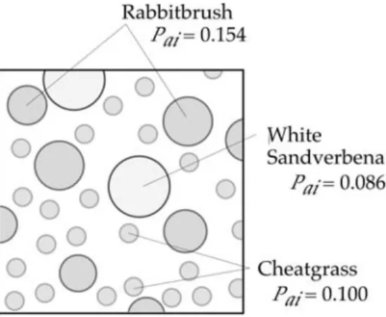
(4) Numerical Simulation of Surface Barriers for Shrub-steppe Ecoregions.. Two fundamental assumptions of this sparse-vegetation evapotranspiration model are that plant canopies do not overlap and that the plant distributions can be described through a plant-species areal distribution (i.e., plant area index). The plant area index describes the fraction of ground surface covered by a particular plant species as shown in Figure 1. The summation of the plant area index over all plant species cannot exceed 1.0, and the difference between 1.0 and this summation equals the exposed ground area index. The more familiar leaf area index refers to the leaf area per footprint of plant area. The governing conservation equations are written with the simplifying assumption that the ground surface beneath a plant species exchanges water mass and thermal energy with the atmosphere via the canopy nodal point, and that the exposed ground surface exchanges water mass and thermal energy directly with atmosphere. A nodal network for the single-plant-temperature option is shown in Figure 2.. Figure 1. Plant area indices for ground surface covered with three species.. Figure 2. Nodal network for the single-plant temperature model. 227.

(5) White and Ward. 2.2.1 Ground-Surface Water-Mass Balance. Within the areal plant distributions (covered), the canopy node intervenes the ground surface to atmosphere connection and outside the areal plant distribution (exposed) the ground surface is connected directly to the atmosphere. The water mass balance equation at the ground surface, therefore, has both canopy and atmosphere components: Ens + Gns egw + Lns elw = Esa + Gsa egw + Lsa elw + Esc + Gsc egw + Lsp elw (1) ns. ns. sa. sa. sc. sp. where, -Lsa represents the precipitation intensity on the exposed ground surface, and -Lsp represents the shed precipitation or condensate intensity from the plants on the covered ground surface. Shed precipitation or condensate occurs when plant leaf water storage capacity is exceeded. The diffusive and advective transport of water between the subsurface and ground surface are conventional expressions for multifluid subsurface flow and transport (White and Oostrom 2000): egw − egw w w w n s ; ew = ω w ρ Ens = τ g nD ρ g s g Dg (2) g g ; eg s = ω g ρ g g n ns n s dzns. (. ⎛ krg k z ⎞ Gns = ⎜ ⎟ ⎜ µg ⎟ ⎝ ⎠ns. ). (. ). (. ). ⎛ Pg n − Pg s ⎞ ⎛ krg k z − g ρ g ns ⎟⎟ ; ⎜ ⎜⎜ ⎜ ⎝ dzns ⎠ ⎝ µg. up krg n , krg s hm k zn , k zs ⎞ ⎟ = ⎟ hm µ g n , µ g s ⎠ns (3) up krln , krls hm k zn , k zs ⎞ ⎛k k ⎞ ⎛ k k ⎞ ⎛ Pl − Pls (4) Lns = ⎜ rl z ⎟ ⎜⎜ n − g ρlns ⎟⎟ ; ⎜ rl z ⎟ = µ µ dz µ µ hm , ns ⎝ l ⎠ ns ⎝ ⎠ ⎝ l ⎠ ns ln ls The ground surface-to-atmosphere and ground surface-to-canopy transport terms take into account the quantity of exposed or covered ground surface: egw − egw ⎛ species ⎞ ega ⎛ species ⎞ i s a ⎜1 − (5) Esa = Pai ⎟ ; Gsa = Gns ans ⎜1 − Paii ⎟ a ⎜ ⎟ ⎜ ⎟ rsa e g sa ⎝ i =1 i =1 ⎝ ⎠ ⎠ egw − egw ⎛ species ⎞ ega ⎛ species ⎞ i s c ⎜ (6) Esc = Pai ⎟ ; Gsc = Gns a sc ⎜ Paii ⎟ a ⎜ ⎟ ⎜ ⎟ rsc e g ns ⎝ i =1 ⎝ i =1 ⎠ ⎠ To determine the three aerodynamic resistances between the ground surface, canopy and atmosphere, thermal stability effects are ignored, allowing a single eddy diffusion coefficient to describe mass and heat transport equally (Campbell 1985). Following van Bavel and Hillel (1976), a momentum roughness height of 0.01 m is used to estimate the wind velocity profile:. ∑. ∑. ∑. u = uref. ∑. ⎛ z + zm ⎞ ⎛ ⎛ zref + zm ⎞ ⎞ ln ⎜ ⎟ ⎟⎟ ⎟ ⎜⎜ ln ⎜ zm ⎝ zm ⎠ ⎝ ⎝ ⎠⎠. 228. −1. (7).

(6) Numerical Simulation of Surface Barriers for Shrub-steppe Ecoregions.. The ground surface to atmosphere aerodynamic resistance is determined by integrating the inverse of the eddy diffusion coefficient over the height range from zm to zref: −1 ⎛ zref + zm ⎞ ⎛ zref + zm ⎞ a 2 (8) rsa = ln ⎜ ⎟ ln ⎜ ⎟ κ uref zm ⎝ 2 zm ⎠ ⎝ ⎠ Above the canopy, the eddy diffusion coefficient is assumed to vary linearly with elevation and friction velocity; below the canopy, the eddy diffusion is assumed to decrease exponentially with height (Shuttleworth and Wallace 1985). Following these assumptions, the aerodynamic resistances of ground surface to canopy and canopy to atmosphere are determined by integrating the inverse of the eddy diffusion coefficient over the height ranges from 0 to dc+z0 and dc+z0 to zref, respectively: −1 ⎤ ⎡ ⎛ ⎛ hc − d c − z0 ⎞ ⎞ ⎞ ⎥ −1 ⎛ a ⎛ 0.4 hc ⎞ ⎢ (9) rsc = ⎜ ⎟ ( exp ( −2.5 ) ) − ⎜⎜ exp ⎜⎜ −2.5 ⎜ ⎟ ⎟⎟ ⎟⎟ ⎥ hc ⎝ Kc ⎠ ⎢ ⎝ ⎠⎠⎠ ⎝ ⎝ ⎣ ⎦. (. ). −1 a ⎡ ⎛ zref + z0 − d c ⎞ ⎤ ⎡ ⎛ zref + z0 − d c ⎞ ⎤ 2 (10) rca = ⎢ ln ⎜ ⎟ ⎥ ⎢ ln ⎜ ⎟ ⎥ κ uref 2 z0 z0 ⎢⎣ ⎝ ⎠ ⎥⎦ ⎢⎣ ⎝ ⎠ ⎥⎦ where, the eddy diffusion at the canopy is computed from the above-canopy velocity profile at the canopy height:. (. ). −1. ⎡ ⎛ zref + z0 − dc ⎞ ⎤ K c = ( hc + z0 − d c ) κ uref ⎢ln ⎜ (11) ⎟⎥ z0 ⎠ ⎦⎥ ⎣⎢ ⎝ Following Monteith (1973), the zero-plane displacement and canopy roughness height are estimated from the canopy height, yielding aerodynamic resistances for uref = 2 m/s, zref = 2 m, zm = 0.01 m, and hc = 0.3 m: s a s a s d c = 0.63 hc ; z0 = 0.13 hc ; rsca = 99.7 ; rca = 38.2 ; rsa = 76.4 (12) m m m Water-vapor density is computed as a function of water-vapor partial pressure and temperature from the steam table formulations (ASME 1967). For the atmosphere, the water-vapor partial pressure is computed from the saturated water-vapor partial pressure (ASME 1967) and relative humidity. For the ground surface, the water-vapor partial pressure is reduced by the soil capillary pressure according to the Kelvin equation:. (. 2. ). ( Pgw )s = ( Psatw (T ))s exp (( Pl − Pg )s. ( ρl R T / M l )−s 1. ). (13). This approach for the water-vapor partial pressure at the ground surface avoids the conventional approach of using a surface resistance (Shuttleworth and Wallace 1985). The aerodynamic resistance between the plant leaves and canopy follows the approach of Stannard (1993): 0.7 w p ρ c p µ cp w p ucf ρ g 2 1/ 2 1/ 3 g g a (14) rpc = ; Nu = Re Pr ; Re = ; Pr = 3 µg ( ke ) g Nu ( ke ) g. (. ). (. 229. ).

(7) White and Ward. where, the wind speed at the mean canopy flow height is determined from the wind speed profile, assuming the mean canopy flow height equal to 1/2 the canopy height: −1. ⎛ hcf + z0 − dc ⎞ ⎛ ⎛ zref + z0 − d c ⎞ ⎞ (15) u = uref ln ⎜ ⎟ ⎜⎜ ln ⎜ ⎟ ⎟⎟ ; hcf = 0.5 hc z z 0 0 ⎝ ⎠⎝ ⎝ ⎠⎠ Precipitation is partitioned between the ground surface and plant leaves according to the plant-area index: ⎛ species ⎞ − La = Lsa + L pa ; Lsa = − La ⎜1 − Paii ⎟ (16) ⎜ ⎟ i =1 ⎝ ⎠ where, precipitation incident on the plant leaves is either intercepted or shed to the ground surface. Precipitation or condensate that forms on the plant leaves is shed from the plants when the stored water exceeds a specified depth that is a function of the plant species dependent maximum dew depth and leaf area:. ∑. ( ) ( i mw p =. d dp. ωlw. ρl Lai Pai. ). i. species. ; mw p=. ∑ ( mwp ). i. (17). i =1. where, the total stored water mass for all species is the summation of the contributions from all species. Condensate forms on the plant leaves whenever the plant temperature falls below the atmospheric dew-point temperature. The condensation rate is controlled by the aerodynamic resistance between the plant leaves and canopy: egw − egw ⎛ species ⎞ p c ⎜ (18) E pc = Paii ⎟ ; egw = ω gw ρ g ; egw = ω gw ρ g a p c p c ⎜ ⎟ rpc ⎝ i =1 ⎠ The rate of water shed from plant leaves to the ground surface is dependent on the incident precipitation, condensate flux, stored water mass and stored water mass capacitance: i ⎡ ⎤ species d d L P E pc mw p ai ai ⎢ ⎥ p Lsp = − max ⎢ − Lsa − w w − w w + , 0 ⎥ (19) ∆t ω l ρ l ω l ρ l ∆t ⎢ ⎥ i =1 ⎣ ⎦. (. ∑. ). ∑. (. (. ). ). 2.2.2 Canopy Water-Mass Balance. Water-mass conservation at the canopy is a steady-flow equation that balances water flux from the ground surface and plant leaves with that released to the atmosphere: Esc + Gsc egw + E pc + Fpc = Eca (20) sc. where, evaporation from the plant leaves to the canopy refers only to water stored on the plant leaves, according to Equation (18). Transpiration from the plant leaves to the canopy includes an additional stomatal resistance, a crop coefficient and a root-stress factor:. 230.

(8) Numerical Simulation of Surface Barriers for Shrub-steppe Ecoregions. −1 ⎞ ⎛ species w w ⎞⎜ i i i ⎛ a i s i⎞ ⎟ ⎛ Fpc = ⎜ eg − eg ⎟ Pai Cc S r ⎜ rpc + rpc ⎟ (21) c ⎠⎜ ⎟ ⎝ p ⎝ ⎠ ⎝ i =1 ⎠ where, the crop coefficient accounts for the yearly growth cycle of the plant species, and the root-stress factor accounts for matric potential across the root depth. The crop coefficient is specified using a five-point yearly cycle and a linear interpolation between cycle points, which allows for the classical crop growing stages: 1) initial, 2) development, 3) mid-season, and 4) late season. The root-stress factor models root-water uptake according to the vertical root distribution and matric potential within the root zone (Jarvis 1989; Vrugt 2001). A one-dimensional root-water uptake model was selected, because it was assumed that the boundary surface area would be greater than the areal plant area, and multiple plants would cover the boundary surface. The root-stress factor depends on the normalized vertical root spatial distribution and soil-moisture stress function (van Genuchten 1987; Brooks and Corey 1964):. ∑(. Sri =. ∫. ζ*. 0. )( ) ( ). 3⎞ ⎛ ⎛ hc (ζ ) ⎞ ⎟ i i i i ⎜ ; γ ( hc (ζ ) ) = 1 + ⎜ 50 ⎟ γ ( hc (ζ ) ) Sd (ζ ) dζ ; Sd (ζ ) = * ⎜⎜ ⎜ h ⎟ ⎟⎟ ζ ⎝ ⎝ c ⎠ ⎠ β i (ζ ) d ζ. β i (ζ ). −1. ∫. 0. (22) where, the soil-water stress function includes the exponent 3, following van Genuchten and Gupta (1993). The fraction of transpired water removed from a subsurface grid block depends on the overall root-stress factor and the normalized vertical root spatial distribution and soil-moisture stress function integrated over the vertical height of the grid block.. 2.2.3 Ground-Surface Thermal-Energy Balance. As with the water-mass balance at the ground surface the thermal-energy balance has both canopy and atmosphere components, that are defined by the plant areal distributions via the plant area index: Rssn + Rsln + Ens hgw + Gns ρ g hg + Lns ( ρl hl )ns + H ns = Esa hgw +. (. ). (. ns. (. )ns. ). Gsa ρ g hg + Lsa ρl hl sa + H sa + Esc hgw sc sa. (. + Gsc ρ g hg. sa. )sc + Lsp ( ρl hl )sp + H sc. (23) The net short-wave radiation to the ground surface considers attenuation by plant leaves and ground-surface reflection, combines the direct and indirect solar radiation contributions, but does not consider multiple reflections: ⎡⎛ species ⎞ ⎛ species ⎞⎤ sn sd ⎢⎜ i ⎟ ⎜ i i i ⎟⎥ Rs = (1 − α s ) Rs 1− Pai + Pai exp −Ce Lai (24) ⎢⎜ ⎟ ⎜ ⎟⎥ i =1 ⎠ ⎝ i =1 ⎠⎦ ⎣⎝ where, the attenuated component of the short-wave radiation follows the equation for plant canopy transmissivity of Goudriann (1998). Long-wave radiation from the sky to the ground surface is computed as a function of the clear-sky emissivity, fractional cloud cover and atmospheric temperature (Campbell 1985):. ∑. ∑. 231. (. ).

(9) White and Ward. ( )a (25). Rsld = ε a0 (1 − 0.84 ca ) σ Ta4 + 0.84 ca σ Ta4 ; ε a0 = 0.741 + 0.0062 Tdp. where, the clear-sky emissivity is an empirical factor that accounts for the difference between atmospheric and clear-sky temperature (Berdahl and Fromberg 1982), and fractional cloud cover is estimated from atmospheric insolation for solar altitudes greater than 10° (Kasten and Czeplak 1980) and (Caroll 1985), otherwise from the previous computed value: 0.294. ⎛ R sd ⎞ 3.75 ⎞ 0 ⎛ (26) ; Risd = ⎜ 0.79 − ca =1.088 ⎜1 − ssd ⎟ I ⎜ R ⎟ θ ⎠⎟ ⎝ i ⎠ ⎝ Solar altitude is computed from the solar hour angle, local latitude and solar declination following Duffie and Beckman (1974) and Llasat and Synder (1998). The downward long-wave radiation is given by Equation (25), modified for plant attenuation per Equation (24). The upward long-wave radiation is a combination of reflected and emitted radiation, but does not consider multiple reflections: ⎡⎛ species ⎞ ⎛ species ⎞⎤ ln ld ⎢⎜ i ⎟ ⎜ i i i ⎟⎥ Rs = ε s Rs 1− Pai + Pai exp −Ce Lai − ε s σ Ts4 (27) ⎢⎜ ⎟ ⎜ ⎟⎥ i =1 ⎠ ⎝ i =1 ⎠⎦ ⎣⎝ The convective-diffusive heat transport between the ground surface and canopy occurs within the areal distribution of plants, and the convectivediffusive heat transport between the ground surface and atmosphere occurs outside the plant cover:. ∑. (. H sc = (Ts − Tc ) ρ g c p g. species. )sc ∑ i =1. (. ∑. Paii. ( ) rsca. i. ; H sa. ). (T − T ) = s a a rsa. ( ρ g c p g )sa. ⎛ species ⎞ ⎜1 − Paii ⎟ ⎜ ⎟ i =1 ⎝ ⎠. ∑. (28). 2.2.4 Canopy Thermal-Energy Balance. Energy conservation at the canopy is a steady-flow equation that balances heat flux from the ground surface and plant leaves with that released to the atmosphere: Esc hgw + Gsc ρ g hg + H sc + E pc + Fpc hgw + H pc = Eca hgw + H ca (29) sc. (. )sc. (. ). pc. ca. where, the convective-diffusive heat fluxes are defined for the areal surface covered by plants:. (. H sc, pc,ca = Ts, p,c − Tc,c,a. species. ) ( ρ g c p g )sc, pc,ca ∑ i =1. (. Paii rsca , pc,ca. ). i. (30). where, the interfacial values of sensible thermal heat capacitance is harmonic averaged.. 2.2.5 Plant-Leaves Thermal-Energy Balance. Energy conservation at the plant leaves is a transient equation that includes the enthalpy of water mass stored on the plant leaves from intercepted precipitation and condensation, 232.

(10) Numerical Simulation of Surface Barriers for Shrub-steppe Ecoregions.. where transpiration is assumed not to contribute to water stored on the plant leaves: R ns p. + R nl p. − L pa ( ρl hl ) pa −. (. ). E pc + Fpc hgw pc. − H pc =. (. ∆ m w hl. )p. ∆t. − Lsp ( ρl hl ) sp − Fpc hlw. np. (31) There are two transpiration flux terms in Equation (45): from plant to canopy, using water-vapor enthalpy, and from subsurface to plant, using liquid-water enthalpy. The latent heat of evaporation for the transpired water occurs at the plant leaves. The interfacial average values for the transpiration terms are donor differenced, depending on the direction of transpiration:. hgw pc. =. hgw for Fpc ≥ 0 p. hgw for Fpc < 0. ;. hlw np. =. c. hlw for Fpc ≥ 0. n w hl p. (32). for Fpc < 0. where, Fpc ≥ 0 implies water supplied from roots, and Fpc < 0, implies stomatal condensation, with water being supplied to the roots. Short-wave radiation into the plant leaves comes from the atmosphere and reflections from the ground surface. Short-wave radiation arriving at the plant leaves is absorbed, reflected, or transmitted. Net short-wave radiation into the plant leaves equals the arriving radiation less the amount reflected and transmitted to the ground surface: ⎛ species ⎞ sn sd su ⎜ R p = Ra + Rs 1 − α i Paii exp −Cei Liai ⎟ (33) ⎜ ⎟ ⎝ i =1 ⎠ where, the upward short-wave radiation from the ground surface includes contributions from inside and outside the areal plant cover: ⎡⎛ species ⎞ ⎛ species ⎞⎤ su sd ⎢⎜ i ⎟ ⎜ Rs = α s Ra 1− Pai + Paii exp −Cei Liai ⎟ ⎥ (34) ⎢⎜ ⎟ ⎜ ⎟⎥ i =1 ⎠ ⎝ i =1 ⎠⎦ ⎣⎝. (. ) ∑ (. ∑. ). ∑. (. ). (. ). Long-wave radiation arrives at the plant leaves from the atmosphere and ground surface, where the ground-surface fraction includes reflected and emitted components. Long-wave radiation arriving at the plant leaves can be absorbed, reflected, or transmitted. View factors from the plant leaves to the ground surface and atmosphere are both assumed to be one. The net longwave radiation at the plant leaves equals the arriving radiation less the amount reflected or transmitted, plus the amount emitted from the plant leaves: Rln p. =. (. species. Rld p. + Rlu p. )∑ i =1. ε i Paii. (. species. ) ∑. ⎡1 − exp −C i Li ⎤ − e ai ⎦⎥ ⎣⎢. i =1. (. ). 2 ε i Paii σ T p 4 ⎡⎢1 − exp −Cei Liai ⎤⎥ ⎣ ⎦. (35) where, long-wave emission is assumed from both sides of the plant. Longwave radiation from the atmosphere is computed according to Equation (25), adjusted for the areal plant cover:. 233.

(11) White and Ward. ⎛ species ⎞ 0 4 ⎤⎜ ⎡ Paii ⎟ (36) = ε a (1 − 0.84 ca ) σ Ta + 0.84 ca σ Ta ⎣ ⎦⎜ ⎟ ⎝ i =1 ⎠ Long-wave radiation arriving at the plant leaves from the ground surface is a combination of reflected long-wave radiation from the atmosphere and that emitted from the ground surface: ⎛ ⎛ species ⎞ ⎛ species ⎞⎞ lu ld R p = Rs (1 − ε s ) ⎜ ⎜1 − Paii ⎟ + ⎜ Paii exp −Cei Liai ⎟ ⎟ + ε s σ Ts 4 (37) ⎜⎜ ⎟ ⎜ ⎟⎟ i =1 ⎠ ⎝ i =1 ⎠⎠ ⎝⎝ where, the amount reflected from the ground surface includes atmospheric radiation from outside and inside the areal plant cover. Root water transported to the plant carries the enthalpy of liquid water at the temperature of the node just adjacent to the boundary surface, following the assumption that root water is in equilibrium with the local node temperature.. ∑. R ld p. ∑. (. ∑. ). 3. Discussion The prototype Hanford barrier is now in its eleventh year of performance testing and monitoring. The first three years compared performance under ambient (170 mm/yr) and elevated (480 mm/yr) precipitation treatments while the past seven years of monitoring have been conducted under ambient precipitation. Data collected over the past 10 years have focused on the water balance components, precipitation, runoff, water storage, and deep drainage with evapotranspiration calculated by difference. Meteorological measurements were made on the barrier and data were collected on the vegetative cover. The measurements focused on species diversity, canopy characteristics including height and leaf area index, and ground cover including root distributions. These data, as well as over 20 years of data from a field lysometer test facility, are being used to calibrate and verify the surface barrier numerical model. Calibration will involve the determination of those critical hydrologic and biotic parameters via inverse modeling where STOMP is coupled to UCODE (Poeter 1998).. Appendix: Nomenclature Roman Symbols ca fractional cloud cover cp specific heat, J/kg K Cc crop coefficient Ce extinction coefficient dc zero-plane displ., m dd maximum dew depth, m D molecular diff. coeff., m2/s e vapor density, kg/m3 E water-vapor flux, kg/m2 s F transpiration flux, kg/m2 s g acceleration of grav., m/s2 G gas flux, m3/m2 s. h hc hc hc50 H I0 ke kr kz K L La Lai 234. enthalpy, J/kg canopy height, m capillary head, m cap. head at 50% reduc., m conv.-diff. heat flux, W/m2 extraterr. solar rad., W/m2 th. conductivity, W/m K phase relative permeability intrinsic permeability, m2 eddy diffusion coeff., m2/s aqueous flux, m3/m2 s precipitation flux, m3/m2 s leaf area index, m2/m2.

(12) Numerical Simulation of Surface Barriers for Shrub-steppe Ecoregions.. mp M nD P Pai ra rs R Rld Rln Rlu Rsd Rsn Rsu s Sd Sr T u z zm z0. stored mass on plant, kg molecular weight, kmol/kg diffusive porosity pressure, Pa plant area index, m2/m2 aerodynamic resist., s/m stomatal resistance, s/m gas constant, J/kmol K long-wave ↓ rad., W/m2 long-wave net rad., W/m2 long-wave ↑ rad., W/m2 short-wave ↓ rad., W/m2 short-wave net rad., W/m2 short-wave ↑ rad., W/m2 phase saturation norm. root spatial distr. root stress factor temperature, K wind speed, m/s elevation, m mom. roughness height, m canopy roughness height, m. Greek Symbols β vertical root spatial distr. ∆t time step, s γ soil-water stress function ε emissivity 0 ε clear-sky emissivity ζ root depth, m. ζ* θ κ µ ρ σ τ ω. maximum root depth, m solar altitude, deg von Karman constant, 0.4 dynamic viscosity, Pa s density, kg/m3 S-B const. 5.67e-8 W/m2 K tortuosity factor mass fraction. Subscripts a atmosphere c canopy cp canopy to plant g gas phase l aqueous phase n subsurface node ns subsurface to ground surf. p plant leaves pa plant to atmosphere ref reference height s ground surface sa ground surf. to atmosphere sat saturated sc ground surf. to canopy sp ground surf. to plant Superscripts a air i plant species w water. References ASME, 1967: Thermodynamic and Transport Properties of Steam, The American Society of Mechanical Engineers, New York. Berdahl, P., and R. Fromberg, 1982: The thermal radiance of clear skies, Solar Energy, 29(4), 299-314. Brooks, R. H., and A. T. Corey, 1964: Hydraulic Properties of Porous Media, Colorado State University, Hydrology Paper, No. 3, Fort Collins, Colorado. Campbell, G. S., 1985: Soil Physics with Basic, Transport Models for Soil-Plant Systems 14, Elsevier, Amsterdam. Carroll, J. J., 1985: Global transmissivity and diffuse fraction of solar radiation for clear and cloudy skies as measured and as predicted by bulk transmissivity models, Solar Energy, 35, 105-118 Duffie, J. A., and W. A. Beckman, 1974: Solar Energy Thermal Processes, A WileyInterscience Publication, John Wiley & Sons, New York. Flerchinger, G. N., and K. E. Saxton, 1989: Simultaneous heat and water model of freezing snow-residue-soil system, I. Theory and development, Trans. ASAE, 32(2), 565-571. 235.

(13) White and Ward. Flerchinger, G. N., and K. E. Saxton, 2000: The Simultaneous Heat and Water (SHAW) Model: Technical Documentation, Northwest Watershed Research Center, USDA Agricultural Research Service, NWRC 2000-09, Boise, Idaho. Goudriann, J., 1988: The bare bones of leaf-angle distribution in radiation models for canopy photosynthesis and energy exchange, Agricultural and Forest Meteorology, 43, 155-169. Jarvis, N. J., 1989: A simple empirical model of root water uptake, Journal of Hydrology, 107, 57-72. Kasten, F., and G. Czeplak, 1980: Solar and terrestrial radiation dependence on the amount and type of cloud, Solar Energy, 24, 177-189. Llasat, M. C., and R. L. Snyder, 1998: Data error effects on net radiation and evapotranspiration estimation, Agr. and Forest Meteorology, 91,209-221. Monteith, J. L., 1965: Evaporation and environment, The State and Movement of Water in Living Organisms, Sympos. Soc. Exper. Biol., edited by G. E. Fogg, 19, 205-234, Academic, San Diego, Calif. Monteith, J. L., 1973: Principles of Environmental Physics, Edward Arnold, London. Penman, H. L., 1948: Natural evaporation from open water, bare soil, and grass, Proc. R. Soc. London, Ser. A. 193, 120-146. Poeter, E. P., and M. C. Hill, 1998: DOCUMENTATION OF UCODE, A Computer Code for Universal Inverse Modeling, U.S. Geological Survey, Water-Resources Investigation Report, 98-4080, Denver, Co. Shuttleworth, J. W. and J. S. Wallace, 1985: Evaporation from sparse crops-an energy combination theory, Quart. J. R. Met. Soc., 111, 839-855. Stannard, D. I., 1993: Comparison of Penman-Monteith, Shuttleworth-Wallace, and Modified Priestly-Taylor evapotranspiration models for wildland vegetation in semiarid rangeland, Water Resources Research, 29(5), 1379-1392. van Bavel, C. H. M., and D. I. Hillel, 1976: Calculating potential and actual evaporation from a bare soil surface by simulation of concurrent flow of water and heat. Agric. Meteorol., 17, 453-476. van Genuchten, M. T. A, 1987: A numerical model for water and solute movement in and below the root zone, Research Report 121, U.S. Salinity Laboratory, Agricultural Research Service, U.S. Department of Agriculture, Riverside, California. van Genuchten, M. T. A., and S. K. Gupta, 1993: A reassessment of the crop tolerance response function, Bulletin of the Indian Society of Soil Science, 4, 730737. Vrugt, J. A., M. T. van Wijk, J. W. Hopmans, and J. Simunek, 2001: One-, two-, and three-dimensional root water uptake functions for transient modeling, Water Resources Research, 37(10), 2457-2470. White, M. D., and M. Oostrom, 2000: STOMP Subsurface Transport Over Multiple Phases, Version 2.0, Theory Guide, Pacific Northwest National Laboratory, PNNL-12030, UC-2010, Richland, Washington.. 236.

(14)

No results found