Using a Geo-statistical Approach for Soil Salinity and Yield
Management
Ahmed A. Eldeiry1 and Luis A. Garcia 2
Department of Civil and Environmental Engineering, Colorado State University
Abstract. This paper presents a practical method to manage soil salinity and yield in order to
obtain maximum economic benefits. The method was applied to a study area located in the south eastern part of the Arkansas River Basin in Colorado where soil salinity is a problem in some areas. The following were the objectives: 1) generate classified maps and the corresponding zones of uncertainty of expected yield potential for the main crops grown in the study area; 2) compare the expected potential productivity of different crops based on the soil salinity conditions; 3) assess the expected net revenue of multiple crops under different soil salinity conditions. Different scenarios of crops and salinity levels were evaluated. Indicator kriging was applied to each scenario to generate maps that show the expected percent yield potential areas and the corresponding zones of uncertainty for each of the different classes. The results of this study show that indicator kriging can be used to generate guidance maps that divide each field into areas of expected percent yield potential based on soil salinity thresholds for different crops. Zones of uncertainty can be quantified by indicator kriging and therefore it can be used for risk assessment of the percent yield potential. Wheat and sorghum show the highest expected yield potential based on the different soil salinity conditions that were evaluated. Expected net revenue for alfalfa and corn are the highest under the different soil salinity conditions that were evaluated.
1. Introduction
Soil salinity refers to the presence in the soil and water of various electrolytic mineral solutes in concentrations that can be harmful to many agricultural crops (Hillel 2000). Salts decrease the availability of water to plants due to increase osmotic potential, and have direct adverse effects on the plant metabolism (Douaik, 2003; Greenway and Munns, 1980). Increasing soil salinity is offsetting a good portion of the increased productivity achieved by expanding irrigation (Postel 1999). On average, 20% of the world's irrigated lands are affected by salts, but this figure increases to more than 30% in countries such as Egypt, Iran and Argentina (Ghassemi et al. 1995). Crop yield reduction in fields in the Lower Arkansas Valley due to salinization is estimated to be 0 to 75% with a total revenue loss ranging from $0-$750/ha based on 1999 crop prices (Gates et al., 2002).
Indicator kriging (IK) provides a non-parametric distribution estimated directly at fixed thresholds by considering indicator transforms of conditioning data in the form of cumulative distribution functions (Richmond 2001). The power of multi-variable indicator kriging as a tool is that it is flexible and can be modified to fit specific management or research goals by modifying the critical threshold criteria (Smith et al., 1993). Indicator kriging makes no assumptions on the underlying invariant distribution, and 0:1 indicator transformation of the data makes the predictor robust to outliers
1 Ahmed A. Eldeiry, Ph.D. Research Fellow, Integrated Decision Support Group, Department of Civil and
Environmental Engineering, Colorado State University, 80523, Phone: (970) 491-7620, FAX: (970) 491-7626, E-Mail: aeldeiry@rams.colostate.edu
2 Luis A. Garcia, Director and Professor, Integrated Decision Support Group, Department of Civil and
Environmental Engineering, Colorado State University, 80523, Phone: (970) 491-5144, FAX: (970) 491-7626, E-Mail: Luis.Garcia@Colostate.edu.
(Cressie, 1993). At an unsampled location, the values estimated by indicator kriging represent a probability that the value is less than a specified threshold. That is, the expected value at the location derived from indicator data is equivalent to the cumulative distribution function of the variable (Smith et al., 1993). Mapping of uncertainty zones for individual phases is one advantage of using a geostatistical approach to characterize the morphology of quantitative variables (Soares 1992). Smoothing effects occurring around zero thickness investigation sites can be reduced significantly by the use of a combined ordinary-indicator kriging approach (Marinoni, 2002). Solow et al. (1986) used simple indicator kriging to estimate the conditional probability that a sample point is one type or other given the types of sample points. Their results show that simple indicator kriging perform well, and in some cases can be exact.
The geostatistical approach presented in this paper uses indicator kriging to provide growers with a tool to evaluate options for obtaining the maximum economic benefit under the current conditions of their fields. For each combination of crops and fields, the soil salinity data for each field was classified into different thresholds to produce the following crop yield potentials: 100%, 90%, 75%, 50%, < 50% & > 0 %, and 0%. Multiphase-variograms were constructed for each of the scenarios and indicator kriging was applied to each scenario to generate maps that show the expected percent yield potential as well as zones of uncertainty for different parts of each field. Expected crop net economic revenue for each scenario was calculated. The expected yield potential maps can be used by growers to determine which crop would maximize the yield and the economic benefits of their fields under the current soil salinity conditions.
2. Data and methodology
Study Area and Data Collection
The study area is located in the southeastern part of the Arkansas River Basin in Colorado near the cities of Rocky Ford and La Junta (Fig. 1). Farmers in this area are facing decreasing crop yields due in part to high levels of salinity in their irrigation water. In some areas, land is being taken out of production due to unsustainable crop yields. Several fields were selected to carry out the soil salinity assessment in the study area. Soil salinity data was collected using an EM-38 electromagnetic probe and a global position systems (GPS) unit. The EM-38 provides vertical and horizontal readings while the GPS unit provides the X and Y coordinates of each collected point. A calibrated equation which was developed for the study area by Wittler et al. (2006) was used to convert the EM-38 readings to EC (dS/m). Soil moisture content and soil temperature were used for the calibration equation. A detailed description of using the EM-38 in combination with GPS in collecting soil salinity and the developed equation can be found in Eldeiry and Garcia (2008) and Eldeiry et. al. (2008). Six fields were selected to represent the different soil salinity ranges: low, moderate, and high.
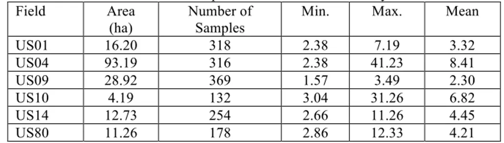
Table 1 shows a description of the fields used in this study. The table contains the area, number of samples, minimum, maximum, and mean of the soil salinity samples. Soil salinity is an important factor which can significantly affect crop yield; therefore, these fields were selected to represent different soil salinity ranges: low, moderate, and high. Table 1 shows that the selected fields represent a wide range of soil salinity levels from 1.57 to 41.23 dS/m.
Figure 1: The study area in the southeastern part of the Arkansas River Basin in Colorado. Table 1: Description of the fields of the study area
Field Area
(ha)
Number of Samples
Min. Max. Mean
US01 16.20 318 2.38 7.19 3.32 US04 93.19 316 2.38 41.23 8.41 US09 28.92 369 1.57 3.49 2.30 US10 4.19 132 3.04 31.26 6.82 US14 12.73 254 2.66 11.26 4.45 US80 11.26 178 2.86 12.33 4.21
Soil Salinity Classification
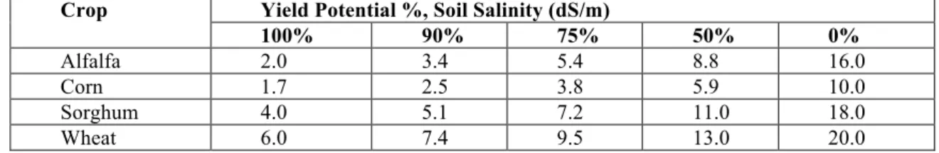
Table 2 shows the percent yield potential and the corresponding soil salinity EC (dS/m) for alfalfa, corn, sorghum, and wheat (adapted from Ayers and Westcot, 1976). The crops shown in Table 2 were sorted based on their tolerance to soil salinity from low to high: corn, alfalfa, sorghum, and wheat. Under the same soil salinity conditions wheat has a 100% yield potential at a soil salinity of 6 dS/m while corn has a 50% yield potential at a soil salinity of 5.9 dS/m. This shows how crops with different soil salinity tolerances have significantly different crop yield potential under the same soil salinity conditions. Therefore, depending on the soil salinity conditions of each field, some crops will have higher yields than others. A classified map of expected yield potential based on soil salinity thresholds of each crop can help in selecting the appropriate crop that maximizes the potential yield for a specific area.
Table 2: Yield potential and the corresponding soil salinity (dS/m) for selected crops (adapted from
Ayers and Westcot, 1976)
Yield Potential %, Soil Salinity (dS/m) Crop 100% 90% 75% 50% 0% Alfalfa 2.0 3.4 5.4 8.8 16.0 Corn 1.7 2.5 3.8 5.9 10.0 Sorghum 4.0 5.1 7.2 11.0 18.0 Wheat 6.0 7.4 9.5 13.0 20.0
Preparing the data
The soil salinity data for each field was sorted and classified into different thresholds to produce the following crop yield potentials: 100%, 90%, 75%, 50%, < 50% & > 0 %, and 0%. For each of the six fields, the classification was done for each of the four selected crops. For high tolerance crops such as wheat or sorghum in fields with low soil salinity levels such as US09; there is no need for indicator kriging since the whole field can produce 100% of the expected yield potential. However, with the same crops in fields with moderate soil salinity levels, crops can reach high yield potential from 100% to 75% while all classes from 100% to 0% can be represented in the fields with high soil salinity levels. For moderate and low tolerance crops, alfalfa and corn, a wide range of yield potentials is represented.
Constructing the multi-phase variograms
From the data combinations of the selected four crops and six fields, twenty four scenarios are created. For each scenario, data is formatted to be able to be read in the S+ statistical software package and the different phases of the variograms are decided based on the number of classes or thresholds of yield potential for each scenario. For example the scenario of planting alfalfa in field US04 has five classes: 90%, 75%, 50%, <50% & > 0%, and 0% of percent of yield potential. The best model variogram among the Exponential, Gaussian, and Spherical is chosen based on the smallest Akaike Information Corrected Criteria (AICC) statistical parameter. Multiphase-variograms were constructed for each of the scenarios using the model with the smallest AICC value. Each phase of the variograms represents one class of percent yield potential. The multi-phase variograms contain six phases or less depending on the tolerance of the crop and the soil salinity in the field. The multi-phase variogram (Soares, 1992) is defined as the probability that and belong to different classes ,
(1) where: and , represent a pair of sample locations separated by distance and
is the number of classes of soil salinity.
Applying Indicator Kriging
IK was applied to each scenario to generate classified maps that show the expected percent yield potential. The number of classes in each map depends on the number of phases of the indicator variograms of that scenario. One of the advantages of IK is that it has the power to quantify the zones of uncertainty for different parts of each field. Zones of uncertainty exist around the borders of classes and these areas have the probability of belonging to either of the classes. Assessing zones of uncertainty can be
very beneficial for the accuracy of the generated maps since it can produce more information about the risk assessment. The essence of the indicator approach is the binomial coding of soil salinity data into either 1 or 0 depending upon its relationship to the thresholds of soil salinity for each crop. For a given value of :
(2) where is the soil salinity threshold for a specific crop (Lyon et. al., 2006). More detailed description of IK can be found in Soares (1992).
Zones of Uncertainty
The indicator variable can be described as the probability of exceeding a given threshold. Therefore, the estimation of the indicator variable at unsampled locations produces probability maps (Reis et. Al. 2005b). Zones of uncertainty between soil salinity classes can be obtained by identifying locations with low probability, for a given threshold, of belonging to a specific soil salinity level. For example we can define a zone of uncertainty as being the lowest 25% of the probabilities of belonging to a particular soil salinity level. To generate a map of uncertainty, the first thing to do is to obtain some information regarding the distribution of probabilities associated with each soil salinity class, such as identifying the threshold representing the lowest 25% of the probabilities.
Consider an attribute Z that must be conditionally simulated and the information available consists of z values at n locations xi, z(xi), i = 1, 2, ... , n. The uncertainty about the soil salinity value at an unsampled location x is modeled by the conditional cumulative distribution function (ccdf) of the random variable Z(x):
(3) The function F(.) gives the probability that the unknown soil salinity does not exceed a threshold z. The ccdfs are modeled using a non-parametric (IK) approach, which estimates the probability for a series of K threshold values zk discretizing the range of variation of Z (Reis et al., 2005a):
(4) where k is the number of samples within a specific class K.
The calculated probabilities are recoded into 0 and 1 in order to obtain binary maps with two levels, the areas with uncertainty and the areas without uncertainly, while considering a confidence interval.
Net revenue
Expected crop net economic revenue for each scenario was calculated based on Colorado State University Extension (Agriculture and Business Management) 2007 crop budget estimates. The total revenue includes the final revenue of the crop without taking into account the costs. The costs include the operations associated with pre-harvest, pre-harvest, property ownership and cost, and for some crops a factor payment. Net revenue is the revenue after the costs are taken into account. The expected crop net
economic revenue can be used as guidance for the growers to determine which crop would maximize the economic benefits of their fields under the current soil salinity conditions.
Model Performance
Indicator kriging performance with the different crops and fields is measures by the following criteria:
1. Model precision: The RMSE is used to measure the prediction precision (Dobermann et. al., 2006; Triantafilis et. al., 2001) and is defined as:
(5) where is the observed value of the ith observation, is the predicted value of the ith observation, and n is the number of collected points.
The RMSE tends to place more emphases on larger errors and, therefore, gives a more conservative measure than the mean absolute error MAE.
2. Smoothing effect: Interpolation usually leads to a smoothing of the observations and thus to a loss of variance. To assess the ability of the interpolation method to preserve the variance, the ratio of the variance of the estimated values to the variance of the observed values is used (Haberlandt, 2006),
(6) The closer RVar approaches 1, the better the ability of the interpolation method to preserve the observed variance.
3. Model effectiveness: The effectiveness of the model was evaluated using a goodness-of-prediction statistic, G (Agterberg 1984; Kravchenko and Bullock 1999; Guisan and Zimmermann 2000; Schloeder et al. 2001). The G-value measures how effective a prediction might be relative to that which could have been derived by using the sample mean (Agterberg 1984),
(7) is the sample mean. A G-value equal to 1 indicates perfect prediction, a positive value indicates a more reliable model than if the sample mean had been used, a negative value indicates a less reliable model than if the sample mean had been used, and a value of zero indicates that the sample mean should be used.
3. Results
This section presents the process of selecting the multi-phase variograms of indicator kriging based on the Akakie Information Corrected Criteria (AICC) statistical parameter. Examples of indicator kriging maps for different scenarios of crops and fields are provided. Examples of zones of uncertainty are presented to quantify the risk associated with each of these zones. Finally, an estimate of the net economic revenue for each of the scenarios is provided.
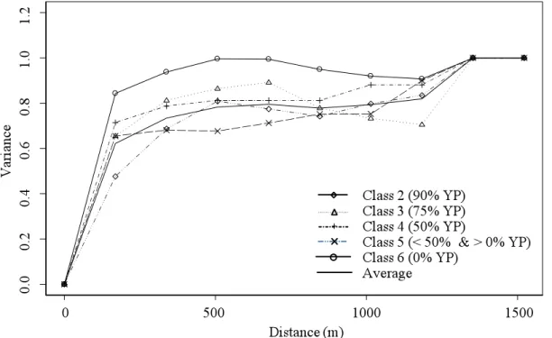
Figure 2 shows an example of the multi-phase variograms for field US04 for a scenario of planting alfalfa. The Gaussian model value has the smallest AICC value; and therefore it was used to construct the multi-phase variogram by sorting the collected soil salinity data for that field from low to high. Then five classes were assigned to the sorted soil salinity data according to the percent yield potential of alfalfa to represent the following yield potentials: 90%, 75%, 50%, < 50% ~ > 0%, and 0%.
Figure 2: Example of multi-phase variograms for field US04 for alfalfa.
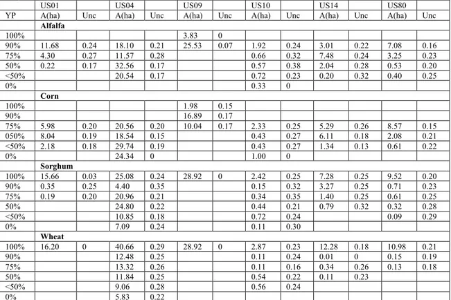
Table 3 shows the yield potential areas of each class and the corresponding zones of uncertainty for all the scenarios of the selected crops and fields. Table 3 shows that fields with low soil salinity ranges (US01 and US09) can reach the maximum production for all crops. However, with moderate and high salinity fields sorghum and wheat start with 100% yield potential areas. Alfalfa has good production and in most scenarios, it starts with 90% yield potential areas. Corn has moderate production and in most cases, it starts with 75% yield potential areas.
Figure 3 shows indicator kriging maps for field US04, with high soil salinity range when the scenarios of planting alfalfa, corn, sorghum, and wheat are applied. Even though field US04 has relatively high soil salinity, the expected production of wheat is relatively high with a large percent of the area represented by 100% and 90% of yield potential. Sorghum and alfalfa expected productions are moderate where the production of sorghum covers all the areas between 100% and 0% while alfalfa covers the areas between 90% and 0% of yield potential. Corn expected production is poor where a few areas are represented by 75% and the majority of areas are represented by 50% or less of yield potential.
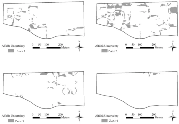
Figure 4 shows an example of zones of uncertainty for field US14 when the scenario of planting alfalfa is applied. One of the advantages of indicator kriging is that it can provide a risk-assessment tool of high-risk regions in the field. Both figure 4 and table 4 show how these areas can be quantified. As shown in table 4, the areas of zones of uncertainty vary between 0% and 35% of the class area.
Table 3: Different classes and zones of uncertainty for the selected fields planted with different scenarios
of growing alfalfa, corn, sorghum, and wheat were evaluated
US01 US04 US09 US10 US14 US80
YP A(ha) Unc A(ha) Unc A(ha) Unc A(ha) Unc A(ha) Unc A(ha) Unc
Alfalfa 100% 3.83 0 90% 11.68 0.24 18.10 0.21 25.53 0.07 1.92 0.24 3.01 0.22 7.08 0.16 75% 4.30 0.27 11.57 0.28 0.66 0.32 7.48 0.24 3.25 0.23 50% 0.22 0.17 32.56 0.17 0.57 0.38 2.04 0.28 0.53 0.20 <50% 20.54 0.17 0.72 0.23 0.20 0.32 0.40 0.25 0% 0.33 0 Corn 100% 1.98 0.15 90% 16.89 0.17 75% 5.98 0.20 20.56 0.20 10.04 0.17 2.33 0.25 5.29 0.26 8.57 0.15 050% 8.04 0.19 18.54 0.15 0.43 0.27 6.11 0.18 2.08 0.21 <50% 2.18 0.18 29.74 0.19 0.43 0.27 1.34 0.13 0.61 0.22 0% 24.34 0 1.00 0 Sorghum 100% 15.66 0.03 25.08 0.24 28.92 0 2.42 0.25 7.28 0.25 9.52 0.20 90% 0.35 0.25 4.40 0.35 0.15 0.32 3.27 0.25 0.71 0.23 75% 0.19 0.20 20.96 0.21 0.34 0.35 1.40 0.25 0.61 0.25 50% 24.80 0.22 0.44 0.21 0.79 0.32 0.32 0.28 <50% 10.85 0.18 0.72 0.24 0.09 0.29 0% 7.09 0.24 0.11 0.30 Wheat 100% 16.20 0 40.66 0.29 28.92 0 2.87 0.23 12.28 0.18 10.98 0.21 90% 12.48 0.25 0.11 0.24 0.01 0 0.15 0.19 75% 13.32 0.26 0.11 0.16 0.34 0.26 0.13 0.18 50% 11.84 0.25 0.54 0.22 0.11 0.23 <50% 9.06 0.28 0.56 0.24 0% 5.83 0.22
YP: Yield potential; Unc.: Zone of Uncertainty percentage.
Figure 3: Indicator kriging maps for field US04 (high soil salinity range) when different crops are
Figure 4: Zones of uncertainty for field US14 for alfalfa.
Table 4 shows the total revenue, cost, and net revenue for alfalfa, corn, sorghum, and wheat based on Colorado State University Extension (Agriculture and Business Management) 2007 crop budget estimates. The total revenue includes the final revenue of the crop without taking into account the costs. The costs include the operations associated with pre-harvest, harvest, property ownership and cost, and for some crops a factor payment. Net revenue is the revenue after the costs are taken into account. The net revenue and costs of alfalfa and corn are high while both are low for sorghum and wheat. For one hectare of alfalfa, in order to gain a net revenue of $1,028, a grower needs to spend $751 while they need to spend only $161 for sorghum in order to gain a net revenue of $220.
Table 4: Total revenue, cost, and net revenue per hectare of alfalfa, corn, sorghum, and wheat
Crop Alfalfa Corn Sorghum Wheat
Total revenue 1,780 1,780 381 863
Cost 751 724 161 403
Net Revenue 1,028 1,055 220 460
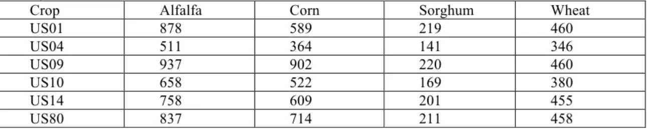
Table 5 shows the adjusted net revenue according to the categorical kriging maps of yield potential of each crop based on the soil salinity thresholds of each field. The adjusted net revenue was calculated as follows,
where n represents the number of different yield potentials classes, i.e. n represents five classes when field US04 is planted with alfalfa.
Table 5: Adjusted net revenue of alfalfa, corn, sorghum, and wheat under the different conditions of soil
salinity at the selected fields.
Crop Alfalfa Corn Sorghum Wheat
US01 878 589 219 460 US04 511 364 141 346 US09 937 902 220 460 US10 658 522 169 380 US14 758 609 201 455 US80 837 714 211 458
The net revenue of the different crops has the following order: alfalfa, corn, wheat, and sorghum. The net revenue of alfalfa and corn are highly affected by the soil salinity levels while sorghum and wheat are slightly affected. Table 3 shows that there is a slight difference between the net revenue of alfalfa and corn while Table 4 shows that there is a significant difference in the adjusted net revenue for alfalfa and corn among different fields due to the tolerance of these crops to salinity and the salinity level for each field. The difference between the net revenue of alfalfa and corn is significant in all fields except for field US09. That is due to the fact that soil salinity in this field allows for 100% of yield potential for corn and there is a big portion of 90% of yield potential for corn while the salinity levels in other fields allows only for 75% or less of yield production for corn.
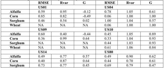
Table 6 shows the performance parameters values of indicator kiging when evaluating alfalfa, corn, sorghum, and wheat as possible crops under the soil salinity conditions of different fields. NA means that the whole field can produce 100% of yield potential which applies to the crops with high tolerance to soil salinity when planted in the fields with low soil salinity levels. The G values are positive for the fields with high and moderate range of soil salinity (US04, US10, US14, and US80) while it getting worse in fields with low range of soil salinity (US01 and US09). In some cases the G value reach 1 or close to 1 which means that the model is perfect such as corn and wheat in US04 and corn in US09. The RVar values are closest to 1 in fields with a high range of soil salinity (US04 and US10). In cases where the RVar values are small such as wheat in US14 and US80, this means that the model was not able to overcome the effects of smoothing. The RMSE values are reasonable acceptable in all fields since all values are equal or less than 1.
4. Conclusions
Soil salinity has the potential to significantly impact crop production. However, soil salinity reclamation is expensive and leached salts may reach ground and surface waters and contribute to pollution. Many growers cannot afford the reclamation costs and sometimes end up having to abandon some fields due to low crop productivity. The findings of this study provide a tool for growers that could help them identify soil salinity problems and assist them in determining what crops to grow based on the soil salinity conditions in order to maximize the economic benefits from their field. Different interpolation techniques such as inverse distance weight, ordinary kriging, simple kriging cannot be utilized to generate categorical maps that show specific areas according to soil salinity thresholds. Indicator kriging can provide this tool where the maps generated can be utilized for any number of specified soil salinity thresholds according to the yield potential of specific crops. Another advantage of indicator
kriging is that it has the power to quantify the zones of uncertainty for different parts of each field. Assessing zones of uncertainty can add a great benefit to the accuracy of the generated maps since it can produce more information about the risk assessment. Indicator kriging can be used as a successful tool for agricultural producers to estimate their yield based on soil salinity conditions. Yield production and net revenue are not in a linear relation due to the significant differences in crop and production prices. Some crops can reach a high yield production under high soil salinity conditions but the net revenue can be low due to the low price of these crops. Some other crops can provide high net revenue with lower yield productivity due to the high price of these crops. Therefore, the approach presented in this study provides growers with a tool to help them decide based on the soil salinity conditions of their fields and their budget what crops they should consider growing.
Table 6: Performance parameters: RMSE, Rvar, and G values of categorical kriging when evaluating
alfalfa, corn, sorghum, and wheat as possible crops.
RMSE Rvar G RMSE Rvar G
US01 US04 Alfalfa 0.59 0.95 -0.12 0.78 1.05 0.61 Corn 0.85 0.82 -0.49 0.06 1.00 1.00 Sorghum 0.46 0.54 0.02 1.00 1.04 0.57 Wheat NA NA NA 0.06 1.00 1.00 US09 US10 Alfalfa 0.60 0.40 -0.44 0.45 1.05 0.89 Corn 0.36 0.99 0.64 0.33 1.04 0.93 Sorghum NA NA NA 0.44 1.03 0.93 Wheat NA NA NA 0.61 1.06 0.84 US14 US80 Alfalfa 0.49 0.77 0.57 0.49 0.90 0.62 Corn 0.40 0.87 0.64 0.44 0.70 0.61 Sorghum 0.73 0.77 0.45 0.69 0.79 0.47
5. References
Agterberg, F.P. (1984). “Trend surface analysis. In ‘Spatial statistics and models”. Ed. G.L. Gaile and
C.J. Willmott 147-171. (Reidel: Dordrecht, The Netherrlands).
Ayers, R. S. and Westcot, D. W. (1976). Water Quality for Agriculture. Irrigation and Drainage Paper 29. FAO, Rome.
Cressie N. Statistics for spatial data. New York: Wiley, 1993.
Dobermann, A. and Ping, J. L. (2004). “Geostatistical Integration of Yield Monitor Data and Remote Sensing Improves Yield Maps.” Agron. J., 96, pp. 285-297.
Douaik A, Van Meirvenne M, Toth T. (2003). “Spatio-temporal kriging of soil salinity rescaled from bulk soil electrical conductivity.” In: Sanchez-Vila X, Carrera J, Gomez-Hernandez J (eds)
Quantitative geology and geostatistics, GeoEnv IV: 4th European conference on geostatistics for enironmental applications, Kluwer Academic Publishers: Dordrecht, The Netherlands, pp. 413–424.
Eldeiry, A. and Garcia, L. A. (2008). “Detecting Soil Salinity in Alfalfa Fields using Spatial Modeling and Remote Sensing." Soil Sci. Soc. Am. J., 72(1), 201-211.
Eldeiry, A., Garcia, L. A., and Reich, R. M., (2008). “Soil Salinity Sampling Strategy Using Spatial Modeling Techniques, Remote Sensing, and Field Data." J. Irrig. Drain. Engin., 134(6), 768-777. Gates, T. K., Burkhalter, J. P., Labadie, J. W., Valliant, J. C., and Broner, I. (2002). "Monitoring and
modeling flow and salt transport in a salinity-threatened irrigated valley," Journal of Water Resources
Planning and Management, 128(2), 87-99.
Ghassemi, F., Jackeman, A. J., and Nix, H. A. (1995). Salinization of land and water resources: human
causes, extent, management and case studies. CAB International, Wallingford Oxon, UK.
Greenway, H., Munns R. (1980). “Mechanisms of salt tolerance in nonhalophytes.” Annu. Rev. Plant
Physiol., 31, 149-190.
Guisan A., and Zimmermann, N. E. (2000). “Predictive habitat distribution models in ecology.”
Haberlandt, U. (2006). “Geostatistical interpolation of hourly precipitation from rain gauges and radar for a large-scale extreme rainfall event.” Journal of Hydrology, 322, pp. 144-157.
Hillel, D. (2000). Salinity management for sustainable irrigation: integrating science, environment, and economics. The World Bank: Washington D.C.
Kravchenko, A., and Bullock, D. G. (1999). “A comparative study of interpolation methods for mapping soil properties.” Agron. J., 91, 393–400.
Lyon, S. W., Lembo Jr., A. J., Walter, M. T., and Steenhuis, T. S. (2006). “Defining probability of saturation with indicator kriging on hard and soft data.” Advances in Water Resources, 29, pp. 181-193.
Marinoni, O. (2003). “Improving geological models using a combined ordinary-indicator kriging approach” Engineering Geology, 69, 37-45.
Postel, S. (1999). Pillar of Sand: Can the Irrigation Miracle Last? W.W. Norton and Co.: New York, NY.
Reis, A. P., Ferreira Da Silva; E., Sousa, A.J., Matos, J., Patinha, C., Abenta, J. & Cardoso Fonseca, E. (2005) - Combining GIS and Stochastic Simulation to Estimate Spatial Patterns of Variation for Lead at the Lousal Mine, Portugal. Land Degradation Development, 16(2): 229-242.
Reis, A.P., Sousa, A.J., Ferreira Da Silva, E. & Cardoso Fonseca, E. (2005) - Application of geostatistical methods to arsenic data from soil samples of the Cova dos Mouros mine (Vila Verde-Portugal). Environmental Geochemistry and Health, 27(3): 259-270.
Richmond, A. (2001). “An alternative implementation of indicator kriging.” Computers & Geosciences,
28, 555-565.
Soares, A., (1992). “Geostatistical Estimation of Multi-Phase Structures.” Math Geol., 24(2), 149-160. Solow, A. R., (1986). “Mapping by Simple Indicator Kriging.” Mathematical Geology, 18(3), 335-351. Schloeder, C. A, Zimmermann, N. E, and Jacobs, M. J. (2001). “Comparison of methods for
interpolating soil properties using limited data”. Soil Sci. Soc. Am. J., 65, 470-479.
Triantafilis, J., Odeh, I. O. A., and McBratney, A.B. (2001). "Five Geostatistical Models to Predict Soil Salinity from Electromagnetic Induction Data Across Irrigated Cotton." Soil Science Society of
America Journal, 65, 869-878.
Wittler, J. M., Cardon, G. E., Gates, T. K., Cooper, C. A., and Sutherland, P. L. (2006). “Calibration of Electromagnetic Induction for Regional Assessment of Soil Water Salinity in an Irrigated Valley.” J.